Functions and water interaction mechanisms of micro/nanostructures on insect cuticle surfaces

Full text

(1)ResearchOnline@JCU. This file is part of the following reference:. Hu, Simon Hsuan-Ming (2014) Functions and water interaction mechanisms of micro/nanostructures on insect cuticle surfaces. PhD thesis, James Cook University.. Access to this file is available from:. http://researchonline.jcu.edu.au/40869/ The author has certified to JCU that they have made a reasonable effort to gain permission and acknowledge the owner of any third party copyright material included in this document. If you believe that this is not the case, please contact [email protected] and quote http://researchonline.jcu.edu.au/40869/.

(2) Functions and Water Interaction Mechanisms of Micro/Nanostructures on Insect Cuticle Surfaces. . By Simon Hsuan-Ming Hu Submitted in total fulfilment of the requirements of the Degree of Doctor of Philosophy School of Pharmacy and Molecular Sciences - James Cook University 2014.

(3) STATEMENT. This work has never previously been submitted for a degree or diploma in any University and to the best of my knowledge and belief contains no material previously published or written by any other person except where due reference is made. Parts of the work described here have been previously published in the following publications: Hu, H. M.; Watson, J. A.; Cribb, B. W.; Watson, G. S. Fouling of Nanostructured Insect Cuticle: Adhesion of Natural and Artificial Contaminants. Biofouling 2011, 27 (10), 1125-1137. Hu, H. M. S.; Watson, G. S.; Cribb, B. W.; Watson, J. A. Non-Wetting Wings and Legs of the Cranefly Aided by Fine Structures of the Cuticle. Journal of Experimental Biology 2011, 214 (6), 915-920. Hu, H. M.; Watson, G. S.; Watson, J. A.; Cribb, B. W. Multi-Functional Insect Cuticles: Informative Designs for Man-Made Surfaces. World Academy of Science, Engineering and Technology 2011, 5 (59), 1370-1371. Watson, G. S.; Hu, S.; Cribb, B. W.; Myhra, S.; Brown, C. L.; Watson, J. A. Micro and NanoStructures Found on Insect Wings - Designs for Minimising Adhesion and Friction. In 2nd International Conference on Advanced Nano Materials; Journal of Nanoscience and Nanotechnology: Aveiro, Portugal 2008; Vol. 8. Watson, J. A.; Cribb, B. W.; Hu, H. M.; Watson, G. S. A Dual Layer Hair Array of the Brown Lacewing: Repelling Water at Different Length Scales. Biophysical Journal 2011, 100 (4), 11491155. Watson, G. S.; Brown, C. L.; Myhra, S.; Roch, N. C.; Hu, S.; Watson, J. A ‘Patterning’ Frictional Differentiation to a Polymer Surface by Atomic force Microscopy - art. no. 60371B. In Device and Process Technologies for Microelectronics, MEMS, and Photonics IV, Chiao, J. C.; Dzurak,. ii.

(4) A. S.; Jagadish, C.; Thiel, D. V., Eds.; Spie-Int Soc Optical Engineering: Bellingham, 2006; Vol. 6037, pp B371-B371.. * ‘Hu, H. M.’, ‘Hu, H. M. S.’ and ‘Hu, S.’ are all initials of Simon Hsuan-Ming Hu. Simon Hsuan-Ming Hu. iii.

(5) ACKNOWLEDGEMENT. This incredible journey has been made possible because of the generous support from many people. The most invaluable guidance came from my University parents Dr. Gregory Watson and Dr. Jolanta Watson. Thanks for unplugging me into the real world and showing me the way of The Force. They have been there for me since before the beginning of this candidature, patiently mentoring me to gain confidence and ambition not just for science but in many aspects of life. Thanks also to Professor Peter Junk for getting me over the line as well as Dr Bronwen Cribb for her expertise in Entomology and Scanning Electron Microscopy and the supportive colleagues and friends from the School of Pharmacy and Molecular Sciences. Lastly thanks to the Graduate Research School for the guidance and the kind scholarship to ease my financial burdens.. iv.

(6) ABSTRACT. Understanding the tribology and adhesion between surfaces at a wide range of length scales is essential for creating the next generation of contamination resistant and super adhesive surfaces. Adhesion and frictional control between solid-solid or solid-liquid surface contacts impact on all aspects of life and is important in a variety of industrial applications and future technologies. Many studies have investigated micro-structures (arrays) on the scale from a few to a hundred micrometres but so far researches on smaller scales have been limited. This study will focus on the contact area and wettability of surfaces on the micro/nanoscale. Insect cuticles, one of the most noteworthy naturally occurring nano-composite materials are considered a free and potentially rich source of technology ‘invented’ by natural selection. Many are multi-functional with efficiencies beyond that of artificially created surfaces. Insects with large wings are unable to clean themselves with their extremities. Contaminants (water and/or contaminating particles) on the wing have a negative effect on the flight capabilities of insects. Insects with a very high wing surface-body mass ratio (SM) index are more susceptible and greatly affected by contamination. A number of these insects exhibit unique structures to decrease wing contamination. Recent studies show that some of these cuticles exhibit impressive superhydrophobic properties. Little was understood about their surface characteristics on the nano-scale prior to the invention of instrumentations and techniques such as the Atomic Force Microscope (AFM) and the Scanning Electron Microscope (SEM). This study utilises the AFM to investigate the tribological properties, including adhesional properties, on a range of insect wing membranes at different length scales. The SEM has been useful to visualise and analyse the nanostructures and properties of surfaces. New methodologies have been employed for micro and nano-scale investigation to determine the functions, functional efficiencies and potential applications of a range of micro/nanostructures recently found on the cuticle of insect wings. Interactions of natural contaminant mimicking spherical surfaces (of different size and chemistry) with insect cuticles were observed and tribological properties were measured. The project will address v.

(7) a number of scientific problems focusing on the control of adhesional properties between surfaces (solid-solid and solid-liquid interactions). A newly discovered water ridding mechanism due to hairs on the lacewing could lead to the creation of a true water repellent surface.. vi.

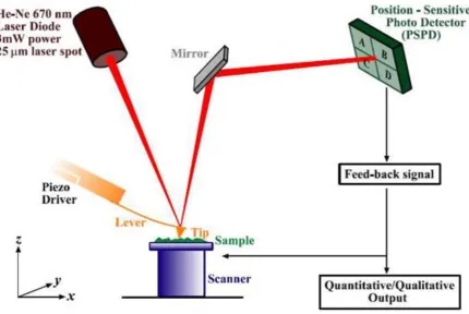
(8) TABLE OF CONTENTS. Statement .................................................................................................................................. ii Acknowledgement .................................................................................................................... iv Abstract ...................................................................................................................................... v Table of Contents ..................................................................................................................... vii List of Figures ............................................................................................................................. x List of Tables .......................................................................................................................... xvii List of Equations .....................................................................................................................xviii List of Abbreviations and Symbols ........................................................................................... xx Feature Article ........................................................................................................................... 1 1. Introduction ....................................................................................................................... 3. 2. Theoretical Background ..................................................................................................... 6 2.1. The Atomic Force Microscope (AFM).......................................................................... 6. 2.1.1. AFM Components & Basic Operations................................................................. 6. 2.1.1.1. The Cantilever & the Tip/Probe .................................................................... 8. 2.1.1.2. Cantilever Loading (Normal) Force Constant ............................................. 10. 2.1.1.3. Cantilever Force Constants Deformation During AFM Operation ............. 12. 2.1.2. Imaging............................................................................................................... 15. 2.1.2.1. Tip Contamination and Breakage ............................................................... 16. 2.1.2.2. Inaccessible Areas during Imaging Operation ............................................ 18. 2.1.3. Lateral Force ...................................................................................................... 19. 2.1.3.1. Friction Loops ............................................................................................. 19. 2.1.4. Force Distance Relation Between Tip and Sample ............................................ 21. 2.1.5. Force Distance Curve and Indentation .............................................................. 25. 2.1.5.1 2.1.6. Indentation and Force Distance Curve on a Soft Surface........................... 25. Capillary Force.................................................................................................... 26 vii.

(9) 2.2. Wettability ................................................................................................................. 28. 2.2.1. Hydrophilicity, Hydrophobicity and Self-Cleaning ............................................. 28. 2.2.2. Contact Angle and Contact Angle Hysteresis..................................................... 29. 2.2.3. Wenzel and Cassie-Baxter Models..................................................................... 31. 2.3. 2.2.3.1. Wenzel Model............................................................................................. 31. 2.2.3.2. Cassie-Baxter (C-B) Model .......................................................................... 32. 2.2.3.3. Stability in The C-B Regime ......................................................................... 34. 2.2.3.4. Applicability of Wenzel and Cassie-Baxter Models .................................... 35. Functional Structured Surfaces ................................................................................. 36. 2.3.1. Functional Structured Surfaces on Insects ........................................................ 37. 2.3.2. Low Adhesion and Self-Cleanig Surfaces ........................................................... 37. 2.3.2.1 2.3.3. Waterproofing Hairs .......................................................................................... 39. 2.3.4. Insect Optical Properties.................................................................................... 40. 2.3.5. Weight and Material Minimisation .................................................................... 42. 2.3.6. Introducing Multifunctionality onto One Surface ............................................. 45. 2.4 3. Antibacterial Surfaces ................................................................................. 38. Chapter Summary...................................................................................................... 46. Experimental Background ................................................................................................ 47 3.1. Atomic Force Microscopy .......................................................................................... 47. 3.1.1. Insect Sample Investigations Using the Atomic Force Microscope ................... 47. 3.1.2 Force distance adhesion and Friction with Contaminants of Various Chemistries and Sizes....................................................................................................... 48 3.1.3. Hair Attachment and Coating ............................................................................ 56. 3.2. Scanning Electron Microscopy (SEM) ........................................................................ 58. 3.3. Photography .............................................................................................................. 59. 3.4. Optical Microscopy.................................................................................................... 59. 3.5. PolyDiMethylSiloxane (PDMS)-A Polymer for Insect Studies ................................... 59 viii.

(10) 4. 3.6. Contact Angle Measurements................................................................................... 60. 3.7. Chapter Summary...................................................................................................... 61. Fouling of Nanostructured Insect Cuticle: Surface Structuring of Cuticle ....................... 62 4.1. Introduction............................................................................................................... 62. 4.2. Topographical Characterisation of Insect Wing Cuticle ............................................ 64. 4.2.1. Super Hydrophobic Cuticles ............................................................................... 67. 4.2.2. Hydrophilic Cuticles ........................................................................................... 68. 4.3 5. 6. 7. Chapter Summary...................................................................................................... 69. Wettability of Nanostructured Cuticles ........................................................................... 70 5.1. Contact Angles and Interaction with Water ............................................................. 70. 5.2. Chapter Summary...................................................................................................... 78. Adhesion of Natural and Artificial Contaminants ............................................................ 79 6.1. Adhesion Force Measurements ................................................................................ 79. 6.2. Chapter Summary...................................................................................................... 87. Non-wetting Wings and Legs of the Cranefly Aided by Fine Structures of the Cuticle ... 88 7.1. Introduction............................................................................................................... 88. 7.2. Results and Discussion .............................................................................................. 89. 7.3. Chapter Summary...................................................................................................... 98. 8 Surface Micro-Structure Flexibility: Advantageous for Lacewing Cuticles Requiring Watering Repelling Mechanisms ............................................................................................. 99. 9. 8.1. Introduction............................................................................................................... 99. 8.2. Results and Discussions ........................................................................................... 101. 8.3. Chapter Summary.................................................................................................... 116. conclusion ...................................................................................................................... 117. 10 References ..................................................................................................................... 120 11 Appendices..................................................................................................................... 134 Other Publications ............................................................................................................. 134. ix.

(11) LIST OF FIGURES. Figure 2.1-1. The path of the laser in a typical AFM instrument reflecting off the cantilever, mirror and onto the detector. ..................................................................... 8 Figure 2.1-2. Reverse image of a 31 m bead revealing a clean surface. ..................... 9 Figure 2.1-3. The relevant force constants of a beam shaped cantilever. .................. 14 Figure 2.1-4. Shows an AFM image where the top half was scanned with a contaminated tip. The contaminant was detached by the scanning procedure around half way through the imaging process and hence the image became more detailed. ...................................................................................................................................... 16 Figure 2.1-1 (A). Double tip resulting in a ghost image to be produced………….……….17 Figure 2.1-5 (B). The end of the tip chips off creating a double tip. ............................ 17 Figure 2.1-6. (A) Shows the tip is unable to reach the bottom of a small hole. (B) The large curved surface does not allow the tip to proceed into it. (C) A tip scans over a bump on the surface and misses a small area beside it. ............................................. 18 Figure 2.1-7. Schematic diagram of a friction loop (A) and the corresponding positions of points 1-6 on the PSPD. A – D represent the four PSPD quadrants. (B) The orange triangles on both (A) and (B) show the tip orientation (see section 1.2.3.3) at the relative positions. (C) Surface motion and its lateral force will cause a tip displacement of xtip which corresponds to an angle of  for a tip with height h. ...................................................................................................................................... 20 Figure 2.1-8. Representative Force distance curve of a tip contacting a hard surface experiencing both attraction and repulsion. ............................................................... 22 Figure 2.1-9. (A) Shape of the cantilever corresponding to section A-B…………………22 Figure 2.1-10. (B) Cantilever jumping into contact with the surface corresponding to section B-C………………………………………………………………………………………………………………22. x.

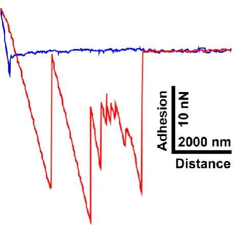
(12) Figure 2.1-10. (C) Shape of the cantilever corresponding to section C-D where an additional loading force is applied………………………………………………………………..…………22 Figure 2.1-10. (D) Shape of the cantilever as it starts to retract from the surface……..23 Figure. 2.1-10.. (E). The. tip. has. detached. from. the. surface………………………………………….23 Figure. 2.1-10.. (F). The. cantilever. retains. its. original. figure…………………………………………23 Figure 2.1-10. F-D curve on a soft PDMS surface (red) calibrated against an F-D curve on a hard surface (orange) to show the amount of indentation at a particular force. ...................................................................................................................................... 27 Figure 2.2-1. The advancing (a) and receding (r) angles of a droplet on a tilted surface.......................................................................................................................... 30 Figure 2.2-2. Droplet in the Wenzel regime. ............................................................... 32 Figure 2.2-3. Droplet in the Cassie-Baxter regime....................................................... 33 Figure 2.3-1. Optical microscope image of microdroplets of water from a mist sprayer supported by hairs on the lacewing Nymphes myrmeleonides. ..................... 40 Figure 2.3-2. Atomic Force Microscope generated 3-D image of a cicada wing array. ...................................................................................................................................... 41 Figure 2.3-3. SEM images of termite wing membrane surface showing star-shaped micrasters and a hair. .................................................................................................. 42 Figure 2.3-4. SEM image of the hair of lacewing showing surface grooves and ultrafine channels at about 45° that meet at the top and bottom of the larger grooves. . 44 Figure 2.3-5. SEM image of the side view of the cicada wing of Gudanga sp. showing the thinner base of the surface structures. ................................................................. 44. xi.

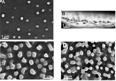
(13) Figure 3.1-1. Insects selected for this work based on their WSA/BM and habits (A) Glenoleon pulchellus (B) Cicadetta oldfieldi (C) Psaltoda claripennis (D) Rhyothemis phyllis chloe. ................................................................................................................. 49 Figure 3.1-2. SEM images showing the orientation of the four types of contaminating particulates attached to AFM levers. (A) Pimelea linifolia ssp., (B) Grevillea ‘Red Sunset’, (C) Acacia fimbriata, and (D) 30 µm silica bead............................................ 52 Figure 3.1-3. SEM images of the finer surface features of the three pollen surfaces used. (A) Pimelea linifolia ssp., (B) Gravillea ‘Red Sunset’ and (C) Acacia fimbriata. . 53 Figure 3.1-4. AFM images of a silica bead, revealing the finer surface structures. (A) A topographical image, (B) a 3-D representation, and (C) an artificially shaded and levelled 3-D image showing the fine surface features. The imaging was performed with the bead attached to a lever and scanned over a calibration grid, i.e., reverse imaging. ........................................................................................................................ 54 Figure 3.1-5. (A) Force distance curve representing the tip at the point of contact with the surface (highlighted with a circle) with a very low indentation force. (B) The surface indenting tip is driven into the surface with a predetermined load hence the longer line (framed in the dotted rectangle) corresponding to sections C-D and D-E of the generic f-d curve shown in Figure 2.1-8. ............................................................... 55 Figure 3.1-6. To avoid meniscus attraction to the hydrophilic lever, the hair was brought into contact to the Milli-Q water droplet from the side of the droplet roughly 500 µm from the top. ..................................................................................... 56 Figure 3.6-1. Venation and regions on an insect wing (example cicada (Psaltoda sp)). ...................................................................................................................................... 61 Figure 4.2-1. Topographical SEM images: (A) & (B) Psaltoda claripennis (top and cross-section, respectively). (C) & (D) Cicadetta oldfieldi (top and cross-section, respectively). (E) & (F) black region of Gudanga sp. nr adamsi (Black cicada) wing membrane (top and cross-section, respectively). (G) & (H) comparable structures found on the dragonfly (Rhyothemis phyllis chloe) and planthopper (Desudaba. xii.

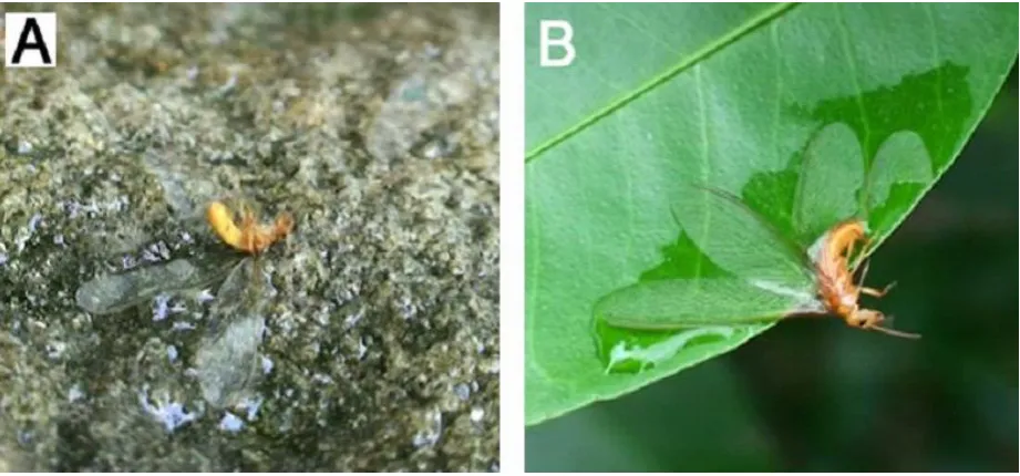
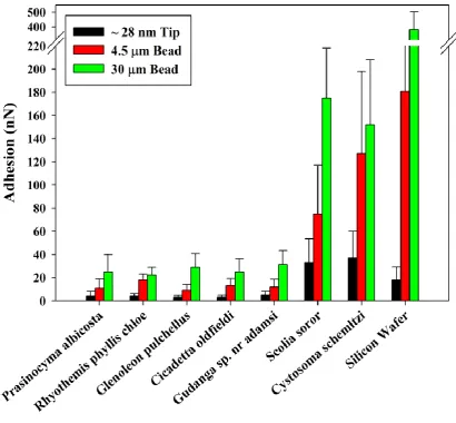
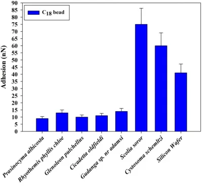
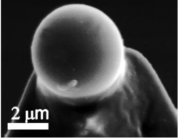
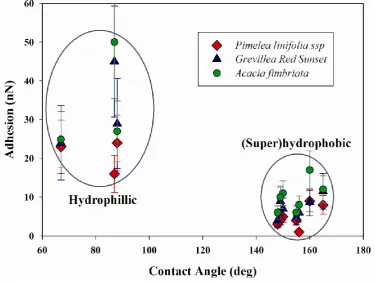
(14) psittacus) wing membranes, respectively. (I) micron, and (J) sub-micron structures found on a moth wing (Prasinocyma albicosta). (K) Lacewing (Glenoleon pulchellus). (L) flower wasp (Scolia soror) nanostructures. (M) Broad bump structuring of the superhydrophilic termite Schedorhinotermes sp.. (N) bladder cicada (Cystosoma schemltzi). .................................................................................................................... 65 Figure 5.1-1. (A) Graph displaying the species type as a function of contact angle ... 71 Figure 5.1-1. A 10 L droplet deposited on (B) a cicada wing membrane, and (C) hydrophobic PDMS surface. (D) & (E) shows the PDMS replica of the cicada Tosena sybilla and the interaction of a water droplet with a polymer (PDMS) replica of the cicada Gaeana cheni respectively…………………………………………………………..……………72 Figure 5.1-2. An optical microscope image of a water droplet resting on the wing membrane of a cicada revealing an apparent contact angle (CA) of ca. 150° with the surface.......................................................................................................................... 74 Figure 5.1-3. SEM images of a PDMS replica of the top (A) and side (B) view of the black cicada (Gudanga sp.) and the top view of the coloured regions found on the cicada wings of Gaeana cheni (C) and Tosena sybilla (D). ........................................... 75 Figure 5.1-4. A ‘fresh’ (A) and dehydrated (B) forewing of the bladder cicada, Cystosoma schmeltzi. ................................................................................................... 76 Figure 5.1-5. (A) and (B) Hydrophilic Schedorhinotermes sp. termite stuck to a wet rock and leaf surface rendering the insect immobilised. ............................................ 78 Figure 6.1-1. Graph displaying the adhesion with the silica particles on the hydrophilic and super/hydrophobic insect wing surfaces. Error bars represent standard errors. ........................................................................................................... 80 Figure 6.1-2 (A). Graph displaying the adhesion with the C18 particles on the hydrophilic and super/hydrophobic insect wing surfaces. Error bars represent standard errors. ........................................................................................................... 82 Figure 2.1-2 (B). SEM image of a C18 bead attached to a cantilever. The section closest to the cantilever tip is contaminated with epoxy and does not interact with the sample……………………………………………………………………………………………………………..82 xiii.

(15) Figure 6.1-3. A single representative F-D curve showing multiple ‘jumps’ on the retract curve (red) obtained on the moth wing (Prasinocyma albicosta). The approach curve (blue) shows a distinct snap-on feature (and a general downward trend) where the Si bead is presumably statically attracted to the surface of the moth scales (since the bead is the object being brought into contact with the surface). ....................................................................................................................... 84 Figure 6.1-4. The overlapping scale arrangement of the Prasinocyma albicosta moth wing. ............................................................................................................................. 85 Figure 6.1-5. Graph displaying the contact angle and adhesion with the three different pollen particles - Pimelea linifolia ssp., Grevillea ‘Red Sunset’ and Acacia fimbriata ‘Golden wattle’. Error bars represent standard errors................................ 86 Figure 6.1-6. A pollen grain found on the wing membrane of the hydrophilic flower wasp, Scolia soror. ....................................................................................................... 87 Figure 7.2-1. (A) Resting cranefly (Nephrotoma australasiae) with a large apparent contact area with the underlying leaf due to the extremely long legs. (B) An ovipositing cranefly at the bottom of the up-down flying pattern on moist/muddy soil showing legs and the tip of the abdomen in contact with the underlying substrate pointing. ....................................................................................................... 89 Figure 7.2-2. Optical images showing a 10 L water droplet displaying superhydrophobic contact on a cranefly (A) wing and (B) leg with the water droplet supported by a syringe to avoid roll off. Micro-sized water droplets from mist sprayer supported by hairs and air underneath and showing superhydrophobicity on the microscale on cranefly (C) wing veins, (D) wing membrane and (E) leg. .................... 91 Figure 7.2-3. (A) SEM images of a cranefly leg with four different types of hair (types a, b, c, d) with nanogrooves visible on hair types a, b and c. (B) SEM images of different size hairs (types e and f) on a cranefly wing (with longer hairs ‘e’ on the wing edge and the veins). (C) High magnification SEM image of cranefly wing showing type ‘f’ hairs. .................................................................................................. 92. xiv.

(16) Figure 7.2-4. SEM image of (A) the fine surface structure found on a small wing hair and (B) leg hair of the cranefly, which show grooves with ultra-fine channels at about 45° which meet at the top and bottom of the larger grooves. ................................... 93 Figure 7.2-5. The hairs which were covered with (A) a thin coating of PDMS still retained a significant amount of the topographical structure (grooves) and (B) a thick coating completely removing the grooves .................................................................. 94 Figure 7.2-6. Optical images showing (A) cranefly hairs on the side of the leg dimpling the water surface (highlighted by arrows). Interaction of individual cranefly hair (type ‘a’) with water. (B) An uncoated hair not penetrating the water surface as observed by the formation of a dimple on the droplet surface from points i to ii. (C) A thinly coated hair also dimpling the water surface. (D) A thick coated hair penetrated the droplet surface. ..................................................................................................... 95 Figure 8.1-1. SEM image of the fine surface structure found on a hair with grooves and ultra-fine channels at about 45° which meet at the top and bottom of the larger grooves....................................................................................................................... 100 Figure 8.2-1. Cells at the tip region which are more elongated and showing higher hair density than the base region (see Figure 8.2-2 for comparison). Hairs generally inclining towards the tip of the wing (right hand side of the image). ....................... 101 Figure 8.2-2. (A) Base region of the lacewing wing observed under an optical microscope showing light Si bead density and bead size range. (B) Typical density of PMMA beads dispersed on the lacewing. ................................................................. 102 Figure 8.2-3. Comparing the effect of hair density on bead removal by Cdrops. The graph shows a higher removal at regions with lower hair densities. ........................ 103 Figure 8.2-4. Comparing the effect of bead removal by the two wetting methods. The difference in the effects is more obvious at high hair density regions where the large drops removes less beads (Figure 8.2-3). .................................................................. 104. xv.

(17) Figure 8.2-5. Hairs prevent wetting of the membrane by water drops landing on the wing. These round drops show low adhesion to the hair can be easily be cleared away by a larger drop rolling past on top of the hair layer. ...................................... 106 Figure 8.2-6. Series of video images showing at [0:00] two droplets (highlighted) on a sample tilted at 45° and coalescing together to the centre of the frame at [2:00] (shadow in [1:00]). At [11:00] has transited to the tip of the hair (shadow in [6:00]) before rolling off at [12:00] after further mist application. ...................................... 107 Figure 8.2-7. Wing cleaned by Cdrops. Beads remain are mostly those near the veins. .................................................................................................................................... 108 Figure 8.2-8. A schematic diagram presenting a Wdrop adhered to the base of the hair on a tilted sample grows in size and detaches from the membrane. ................ 109 Figure 8.2-9. (A) Highlighted drops at [0:00] coalesces and becomes a Cdrop in [1:00] (red line added to show movement). Another Wdrop-Cdrop transition on the left at [6:00] where the highlighted drop in [5:00] combines with a drop behind it........... 110 Figure 8.2-9. (B) A schematic diagram presenting a Wdrop to Cdrop transition on a sample laid flat. The Wdrop is squeezed by the contacting hairs as it grows in size……………………………………………………………………………………………………………..…………111 Figure 8.2-9.(C) The larger highlighted drops at [0:00] coalesces with a drop behind. Picks up the other highlighted drop as it moved to the top right corner of the frame in [1:00] and [10:00]. Detaches and rolls off at [20:00] after further mist plication………………………………………………………………………………………………..………………111 Figure 8.2-10. Comparing the effect of bead size on removal by Cdrops. At high hair density the difference is more prominent. ................................................................ 112 Figure 8.2-11. Side view optical microscope images showing microdroplets on a Micromus tasmaniae wing. The droplets maintain their spherical shape and occupy regions between the macrotrichia arrays, that is, on the microtrichia. .................... 115. xvi.

(18) LIST OF TABLES. Table 3.1-1. Dimensional parameters with standard errors of the artificial particles used for adhesion measurements. The values are averaged for 5 particles per particle type (35 in total)......................................................................................................................................... 50 Table 2.1-2. Dimensional parameters with standard errors of the pollen particles used for adhesion measurements. The values are averaged for 5 particles per particle type (35 in total)……………………………………………………………………………………………………………………………….….50 Table 4.2-1. Geometrical parameters of cuticles from insect species investigated in this study......................................................................................................................................... 66. xvii.

(19) LIST OF EQUATIONS (. ) (. ). (. ) (. ). kN . Equation 2.1-1………………………………………………………………………………………..7 Equation 2.1-2………………………………………………………………………………………..7. Et 3 w Equation 2.1-3 ..................................................................................................... 10 4 L3 1.  3  2 k N  2 L w    03 Equation 2.1-4 ............................................................................... 11  E  3 3. 1 . 1 2. kN . kN M  0.2427m. Equation 2.1-5 ............................................................................... 11. K0 Equation 2.1-6 .............................................................................................. 11 C / D 1. k N   k N. 3L Equation 2.1-7 ............................................................................................ 12 L. kL . k N L2 Equation 2.1-8 ...................................................................................................... 13 3h 2. kT . Gwt 3 Equation 2.1-9 ..................................................................................................... 13 3Lh 2.  2 L2  kT  k N  2  Equation 2.1-10.................................................................................. 13  3 1    h  kCb. w2  k N 2 Equation 2.1-11 ................................................................................................. 14 t. kCsx  Gx t. w2 Equation 2.1-12................................................................................................ 14 L. kCsz  Gz t. w2 Equation 2.1-13 ............................................................................................... 15 L. FL  kT xTip Equation 2.1-14 .................................................................................................. 21 xviii.

(20) FN  k N. [adhesion force   final det ector value – initial det ector value ] Equation 2.1-15 …25 C. 2 E * 2 Fcone ( )   tan . Equation 2.1-16 ....................................................................................... 25. 1  2 1 1  tip 1   sample    E* Etip Esample Esample 2. cos 0  . (  SV –  SL )  LV. 2. Equation 2.1-17 ............................................................ 26. Equation 2.2-1 ............................................................................. 28. CAH   a   r Equation 2.2-2 .......................................................................................... 30. Force ~  LV (cos  r - cos  a ) Equation 2.2-3............................................................... 30 r. cos rough _ surface cos W actual _ surface   geometric _ surface cos smooth _ surface cos 0. Equation 2.2-4 ............................... 31. cos c  f1 cos 0  f air cos  air Equation 2.2-5............................................................ 32 cos c  f1 cos 0  f air Equation 2.2-6 ......................................................................... 32 cos C  rf1 cos 0  f1  1 Equation 2.2-7 ..................................................................... 33 cos  0 . 1  f1 Equation 2.2-8 ........................................................................................... 34 f1  r. 2 C  cos 1  1  B  cos  0  1  Equation 5.1-1 ................................................................... 73. . . F  2 R (1  cos 0 ) Equation 6.1-1........................................................................... 7988. xix.

(21) LIST OF ABBREVIATIONS AND SYMBOLS . half angle of the tip. AFM. atomic force microscope. C. slope of approach curve of the cantilever pushing against an incompressible surface. CA. contact angle. CAH. contact angle hysteresis. D. deflection of the cantilever. ddH2O. double-distilled water. xtip . tip displacement. E. Young’s Modulus. E*. Relative Young’s Modulus. Esample. Young’s Modulus of the sample. Etip. Young’s Modulus of the tip. . angle of tip displacement. F. meniscus force between a sphere and a flat surface. f1. the surface area fraction under the droplet in contact with the solid substrate. fair. tip displacement as an angle of twist. . ratio of the basal area of the protrusion over the total area. Fcone. loading force from a cone shaped tip. F-D. force distance. FL. lateral loading force of the AFM cantilever. FN. normal loading force of the AFM cantilever. FSTW. solvent adhesive forces. FvdW. van der Waal forces. G. shear constant. . solid-vapour interfacial energies/tensions. LV. solid-vapour interfacial energies/tensions. SL. solid-liquid interfacial energies/tensions. xx.

(22) SV. liquid-vapour interfacial energies/tensions. h. height of tip. IA. intensity of the light received by quadrant A of the PSPD. IB. intensity of the light received by quadrant B of the PSPD. IC. intensity of the light received by quadrant C of the PSPD. ID. intensity of the light received by quadrant D of the PSPD. k. cantilever spring constant of the bending of the cantilever in the z-direction. k0. contributing to the tip displacement in the y-direction. kCb. cantilever spring constant of the shear deformation of the tip in the x-direction. kCsx. cantilever spring constant of the shear deformation of the tip in the z-direction. kCsz. standard cantilever spring constant. kL. lateral force constant of the AFM cantilever. kN. normal force constant of the AFM cantilever. kT. twisting force constant of the AFM cantilever. L. cantilever length. M. end mass. m. mass of beam cantilever. . Poisson’s ratio. PDMS. polydimethylsiloxane. PMMA Poly[methyl methacrylate] PSPD. position sensitive photo-detector. 0. static CA formed with a smooth surface. a. advancing contact angle. air. CA formed with air = 180°. c. static apparent CA of a droplet in the Cassie-Baxter regime. r. receding contact angle. w. static apparent CA of a droplet in the Wenzel regime. . material density. r. roughness. R. tip radius. r2. roughness on surface features (secondary roughness). xxi.

(23) RH. relative humidity. . indentation. SEM. scanning electron microscope. SM. surface body mass ratio. t. cantilever thickness. . resonance frequency of the cantilever. . perturbs the resonance frequency of the cantilever. w. cantilever width horizontal position of the centre of the light spot with respect to the centre on the. X. quadrant detector vertical position of the centre of the light spot with respect to the centre on the. Y. quadrant detector. . xxii.

(24) FEATURE ARTICLE INSIDE JEB (March 15, 2011). NON-STICK HAIRS KEEP CRANEFLIES DRY. Large animals think nothing of walking through a heavy mist: water droplets simply role off their hides. However, smaller insects are at constant risk of entrapment by the sticky forces of surface tension. Craneflies, which set up home in boggy settings and riverbanks, routinely 1.

(25) encounter damp surfaces and mist that could prove fatal, yet they shrug off droplets with ease and can even stand on water. Jolanta Watson and colleagues from James Cook University and the University of Queensland, Australia, decided to take a close look at the insect's fragile legs and wings to find out how craneflies avoid getting stuck in water. Photographing cranefly legs at increasing magnification, the team could see that the insect's legs are covered with water-repelling hairs: thick long (90 μm) hairs with a rough grooved surface, shorter thick curved hairs, even shorter fine hairs and the shortest hairs of all found clustered at the base of the longest thick hairs. The insect's wings are also covered in fine hairs, with 12 μm long hairs distributed evenly across the membrane and 90 μm long hairs coating the wing veins. To find out how repellent the hairy surfaces are, the team photographed water droplets on the insect's legs and wings. They saw that instead of spreading over the insect, the droplets formed perfect spheres, characteristic of the way water is repelled by a hydrophobic surface. And when they laid a cranefly leg on water, the hairs formed tiny dimples in the surface instead of piercing it. Finally, the team tested how the grooves on the longer hairs help the insects repel water by coating the long hairs with hydrophobic polydimethylsiloxane to fill the grooves. Poking coated and uncoated hairs into water droplets, the team could see that the coated hairs no longer repelled water and penetrated the droplets with ease, while the uncoated hairs were unable to pierce the droplets. So craneflies avoid getting trapped in sticky water with a coating of rough hydrophobic hairs. Watson and her colleagues are keen to design cranefly-inspired water-repelling and self-cleaning surfaces. (See Chapter 7). 2.

(26) 1. INTRODUCTION. The promise of controlling the tribology and adhesion between surfaces at various length scales, and more importantly an advanced understanding of the processes involved, will ultimately lead to the next generation of contamination resistant and super adhesive surfaces (Blossey, 2003). Adhesion and frictional control between surfaces, whether as solid-solid or solid-liquid contacts, impact on all aspects of life from the need to keep surfaces clean, to the state-of-the-art of droplet-based micro-fluidics systems (Blossey, 2003, Lehto et al., 1999). The Holy Grail in regards to adhesion would be the ability to fabricate surfaces at two extremes - a surface that adheres to anything and a surface that nothing will adhere to. Controlling adhesion between solid-solid and solid-liquid contacts is critical in a number of industrial applications and more important for predicted future technologies. For example, advances. in. nanotechnology,. including. micro/nanoelectromechanical. systems. (MEMS/NEMS) has stimulated development and the need to design surfaces with ultra-low adhesion (Burton and Bhushan, 2005). When considering the functionalities of micromechanical and nano-sized devices that require materials with tailored tribological properties, the issues addressed in this project become more critical (Burton and Bhushan, 2005). The contact area and wettability will affect the adhesion, friction and wear, and may inhibit, possibly prohibit, the functionalities of micromechanical and nano-sized devices, as well as impact on their ultimate life expectancy (Burton and Bhushan, 2005, Abdelsalam et al., 2005, Ando and Ino, 1998). Many studies have investigated well-ordered structures (arrays) on the scale from a few to a hundred micrometres. However, so far there have been only a limited number of studies of nm-sized structures (Burton and Bhushan, 2005). Naturally occurring nano-structures are a much-neglected, but potentially rich, source of products exhibiting finely tuned functional efficiencies. While the pharmaceutical industry has long recognized the value of natural compounds, the emerging industries based on nanotechnology have so far made relatively little use of ‘free’ technology that has been ‘invented’ by the imperatives of species survival. One of the most noteworthy naturally occurring nano-composite material is the insect cuticle (Vincent and Wegst, 2004). Many 3.

(27) micro/nano-structures found on cuticles of insects are multi-functional and some have efficiencies beyond that of artificially created surfaces. Recently natural micro- and nanostructures found on insect cuticles have been shown to exhibit a range of impressive and remarkable properties such as superhydrophobicity, directed wetting and ultra-low adhesion (Parker and Lawrence, 2001, Gorb et al., 2000, Watson et al., 2008b). A study and seminal work by Wagner et al showed that there was a correlation between contaminability, wettability and the wing area of many insects (Wagner et al., 1996). They showed that large winged insects such as butterflies demonstrated extremely low contamination and have very unwettable wings, while smaller winged insects (e.g., flies) showed the opposite trend. Additional weight due to contamination (water and/or contaminating particles) can potentially have a detrimental effect on the flight capabilities of large wing insects (Wagner et al., 1996). Insects with a very high wing surface-body mass ratio (SM) index will have an even greater susceptibility to these effects. A number of insects which have large wings and/or high SM values exhibit unique structures to combat wing contamination from foreign bodies such as water and particulates (Gorb et al., 2000, Fang et al., 2007, Large et al., 2007, Tada et al., 1998) . The result in most instances provides an extremely hydrophobic and in some cases superhydrophobic surface. These superhydrophobic surfaces will not only reduce the effects of contact with particulates but also promote other functional properties (Watson et al., 2008b) such as self-cleaning for removing foreign bodies such as dust (Wagner et al., 1996). The mechanisms and functional efficiency of nano-structures identified on a variety of insects has as yet not received a great deal of attention. One of the major obstacles to a better understanding of these structures has been the inability to undertake surface and interface characterization on the nano-scale. The invention of instrumentation and techniques such as the Atomic Force Microscope (AFM), and the latest generation of imaging and analytical electron-optical techniques has given the scientific community new tools with which to visualise and analyse the structure and properties of surfaces and interfaces on the nano- and meso-scale. In this study the latest instrumentation and methodologies for nano and micro-scale investigation was utilized in order to determine the function, functional efficiency and 4.

(28) potential applications of a range of novel nano- and-micro scale structures recently discovered by Watson et al. (Watson et al., 2008b, Watson and Watson, 2004, Watson et al., 2007) and by others (Wagner et al., 1996) on the cuticle of insect wings. In particular, this study will utilise the AFM to investigate the tribological properties including adhesional properties on a range of insect wing membranes at different length scales. A previously unreported water ridding mechanism is included in Chapter 8. Understanding surface functional mechanisms provides clearer directions towards creating new and more efficient surface functionalities to help meet the standard and demands of upcoming nanotechnologies. Information required prior to the experiments are contained in Chapter 2 and 3. Chapter 4, 5 and 6 investigate the insect wing structures on a range of species and their nano, micro and macro scale properties particularly wetting (Chapter 5) and adhesion with solids (Chapter 6). Chapter 7 highlights the importance and efficiency of surface structures in nonwetting of the hairs on craneflies. Moving onto a larger insect for a more in-depth investigation of the role of cuticle hairs Chapter 8 examines the mechanistic processes involved in wetting prevention, self-cleaning and water repelling by the hairs on lacewing cuticles.. 5.

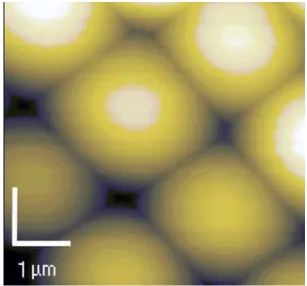
(29) 2. THEORETICAL BACKGROUND. 2.1 THE ATOMIC FORCE MICROSCOPE (AFM) The Atomic Force Microscope (AFM) is a sub-family member of Scanning Probe Microscopy (SPM) and in its early days was typically used for imaging beyond the optical microscope limit. However, its unique imaging method of using a probe to interact with the sample surface allows other surface features/properties to be determined. The AFM’s potential as a force sensing instrument on surfaces is a significant factor contributing to its popularity. The basic elementary function common to all SPMs is using the probe to interact with surfaces. At high resolutions this interaction can occur primarily between several atoms on the apex of the tip and atoms on the surface. The amount of interaction can be plotted as a function of the lateral position to produce an image. Its unique imaging method of using a probe to interact with the sample surface allows other surface properties such as surface adhesive forces, frictional forces and material spring constants (Gibson et al., 1997, Watson, 2001) to be determined as well as surface manipulation (Watson et al., 2006a, Watson et al., 2008c, Watson, 2005).. 2.1.1 AFM COMPONENTS & BASIC OPERATIONS Typically the main elements of the AFM consist of the laser, detector, scanner and most importantly the probe. The probes consist of a cantilever and tip which constitutes the interface between the sample and the other components of the AFM. The other two important components of the AFM are the laser and the position-sensitive-photo-detector (PSPD) which combine to monitor the deflection of the cantilever. During the AFM operation, the laser reflects off the top surface of the cantilever and its intensity is received typically by the four quadrants on the PSPD. The amount of intensity each quadrant receives during scanning will constantly change as the tip interacts with the sample surface.. 6.

(30) Generally for imaging the tip is held in contact with the surface, with a piezoelectric scanner responsible for moving the sample or the probe in a raster pattern during the process of operation. Most AFM instruments allow the user to set various scanning parameters: scan speed, scan area; resolution (i.e., increment in the y-direction), scan angle, response sensitivity (feedback) etc. As the tip moves over a structure, the cantilever will bend, buckle and/or twist corresponding to any change in topography height, adhesion and surface friction. The software converts the cantilever movements into a topographical image or a surface force map. The PSPD implemented in the instrumentation used in this thesis is composed of four separate quadrants (ABCD (Figure 2.1-1)) where the position of the centre of the laser is determined from the relative intensities received by the quadrants. The top and bottom part of the PSPD (AB and CD respectively) detects bending (and buckling in some cases) of the cantilever which corresponds to changes to the sample topography given by Equation 2.1-1. (. ). (. ). Equation 2.1-1 Where Y is the vertical position of the centre of the light spot with respect to the centre on the quadrant detector and IA, IB, IC and ID are the intensities of the light received by each of the quadrants A, B, C and D respectively. Similarly, the quadrant pairs AC and BD measure the lateral twisting of the cantilever due to the frictional/lateral forces with the sample given by Equation 2.1-2. (. ). (. ). Equation 2.1-2 Where X is the horizontal position of the centre of the light spot with respect to the centre on the quadrant detector. 7.

(31) Figure 2.1-1. The path of the laser in a typical AFM instrument reflecting off the cantilever, mirror and onto the detector.. 2.1.1.1 THE CANTILEVER & THE TIP/PROBE Interaction with the sample surface is probed at the free end of a cantilever. Cantilevers are available in a wide range of dimensions/shapes, chemistries and stiffnesses. Most of the cantilevers consist of a sharp tip at the free end. The tips are also commercially available in a wide variety of dimensions/shapes and chemistries. Choosing between the wide range of AFM probes will depend on the purpose and the surface being scanned. Beam shaped cantilevers were predominately used for the studies in this thesis (Figure 2.1-3) (discussed in greater detail in sections 2.1.1.2, 2.1.1.3). V-shaped cantilevers were designed to minimise twisting and improve topographical imaging quality, however Sader (Sader et al., 2003) suggests that V shaped cantilevers actually twist more than beam shaped cantilevers. Tipless cantilevers can be employed for attachment of particles of specific sizes and chemistry both anthropogenic and natural in origin. For example, particles such as pollen and silica beads which mimic natural contaminants can be 8.

(32) attached to tipless cantilevers under an optical microscope (Section 3.1.3 for hair attachment procedure). The particles can be characterised by scanning over an array of spikes (with radius << radius of beads) i.e. reverse-imaged (Hellemans et al., 1991) (Figure 2.1.2). Resonance frequency measurements can be carried out prior and after their attachment to measure other parameters such as spring constants.. Figure 2.1-2. Reverse image of a 31 m bead revealing a clean surface.. The deflections of the cantilever due to any surface features allow a topographical image or a map of the force (e.g., frictional) to be produced. The bending (in the z-direction) and twisting (in the x-direction) of the cantilever corresponds predominantly to changes in topography and the surface friction, respectively (refer to Figure 2.1-3 for the directions). The choice of cantilever force constants will depend on the surface being scanned and the magnitude of the interacting forces. During imaging in the common constant force mode, a feedback system responds to the deflections of the lever to maintain constant loading force by moving the probe up or down to counter the deflection due to a bump or depression, respectively. For contact mode imaging keeping a constant loading force is important in both topographical and lateral 9.

(33) scanning. If the force exerted on the surface is great enough, manipulation of the surface and the creation of structures on the micro and nano-scale can occur (Watson et al., 2006b).. 2.1.1.2 CANTILEVER LOADING (NORMAL) FORCE CONSTANT The spring constant (kN) is dependent on the cantilever’s dimensions and material properties. Obtaining kN is especially important in the force-distance operation (Sections 2.1.4 and 2.1.5). Silicon nitride and silicon are two of the most common materials for probes. For a beam-shaped cantilever with dimensions (length, width and thickness (L, w, t)) and Young’s Modulus (E) (= 130 Gpa for Si (Hopcroft et al., 2010)) the spring constant is:. Et 3 w kN  4 L3 Equation 2.1-3 V-shape cantilevers are often approximated as two parallel beams and Equation 2.1-3 becomes. Et 3 w kN  2 L3. where L in this case is the distance of the tip from the cantilever. (Sader, 1995). Measuring the lever parameters like cantilever thickness (typically a few m) to a high accuracy requires the Scanning Electron Microscopy (SEM). Reflective or additional coatings of different physical properties on cantilevers can alter the spring constant (by less than 0.005N/m for the cantilevers used in the experimental sections). There are methods which reduce or eliminate the power of the dimension terms by introducing other terms such as the resonance frequency of the cantilever (0) and cantilever material density (). The resonant frequency of the cantilever is also dependent on the cantilever’s dimensions and density of its material and hence can be used to replace the thickness term in Equation 2.1-3. The spring constant of a beam shaped cantilever can be obtained using Equation 2.1-4: 1.  3  2 k N  2 L w    03  E  3 3. 10.

(34) Equation 2.1-4 Where  = 2340kg/m3 (in this case for Si) (Watson, 2005). For non-tipless cantilevers (where L/w > 5) (Sader et al., 1999)), the extra weight (M) due to the tip perturbs the resonance frequency measurement to become 1 (Harris and Crede, 1976, Jing et al., 2007):. 1 . 1 2. kN M  0.2427m Equation 2.1-5. for an extra mass of. 1/3 of the beam lever,  could be dampened by. 15% and hence. reducing kN by 34%. Static loading methods are simple and direct and are applicable to various cantilevers and can also be used to measure the stiffness of microtrichia (small hairs on the wings and bodies of insects), as described in greater detail in Section 3.1.2. The cantilever’s deflection due to a known loading force applied above the cantilever tip is obtained to determine the spring constant according to Hooke’s law (Force = kN X deflection). Using an AFM with a calibration cantilever (with a well determined ‘known’ spring constant) an unknown cantilever’s force constant can be accurately determined using force-distance (f-d) curves. The slope of the curve D represents the deflection of the cantilever and hence kN is given by (Gibson et al., 1996):. kN . K0 C / D 1 Equation 2.1-6. where K0 is the standard cantilever spring constant and C is the slope of the cantilever pushing against an incompressible surface (slope of approach curve 1, Figure 2.1-10). The accuracy depends on the precision of the loading force and the point of loading which is associated with the dexterity, judgement and experience of the operator (Gibson et al.,. 11.

(35) 1996) however accuracy is generally lower for cantilevers with low spring constants (i.e. kN < 1N/m) (Butt et al., 2005, Ying et al., 2007). For beam shaped cantilevers, the inaccuracies can be reduced by taking deflections due to loading forces applied along the cantilever(Ying et al., 2007). The offset in the loading point L on a beam cantilever will cause the spring constant to change by kN approximated by (Ying et al., 2007):. k N   k N. 3L L Equation 2.1-7. for |L| << L. An image of the loading point allows the location to be chosen close to the tip of the unknown cantilever. The unknown cantilever should have a spring constant within an ideal range between (Gibson et al., 1996) 0.3K0 to 3.0K0,. Using several cantilevers within that spring constant range for calibration will improve accuracy. Other alternative methods of determining spring constants include measuring the resonance frequency under different density liquids (Sader et al., 1999) or with a known mass attached (Harris and Crede, 1976, Jing et al., 2007). In the experiments involved in this thesis, resonance and static loading techniques using pre calibrated cantilevers were utilised to accurately determine cantilever and hair spring constants, respectively. As well, whenever possible, measurements on several different surface samples were taken using the same set of cantilevers under the same conditions to compare adhesion values.. 2.1.1.3 CANTILEVER FORCE CONSTANTS DEFORMATION DURING AFM OPERATION Bending, buckling and twisting of the cantilever are an important part of the AFM operation. These deformations are results of tip interactions with the local forces of the sample. 12.

(36) surface. Forces acting along the z-, y- and x-direction correspond to the bending (in the normal direction), (longitudinal) buckling and twisting of the cantilever, respectively. The bending of the cantilever in the z-direction (as discussed above) will also contribute to the tip displacement in the y-direction. The force constants kN, kL, kT shown in Figure 2.1-3 are given by Equation 2.1-3 (Section 2.1.1.2), Equation 2.1-8 and Equation 2.1-9 (Gibson et al., 1997, Ogletree et al., 1996, Warmack et al., 1994) which describes the deformation of the lever by the lowest order modes of a long thin beam:. k N L2 kL  2 3h Equation 2.1-8. Gwt 3 kT  3Lh 2 Equation 2.1-9 where h is the height of the tip, G is the shear constant of the cantilever = E[2(1   )]1 (Watson, 2005) andis the Poisson's ratio (≈0.4 in this case for Si)(Watson, 2005). If the normal spring constant of the probe is known then the lateral twisting force constant can be calculated using Equation 2.1-10:.  2 L2  kT  k N  2  3 1    h  Equation 2.1-10. 13.

(37) Figure 2.1-3. The relevant force constants of a beam shaped cantilever.. The bending of the cantilever in the z-direction will also contribute to the tip displacement in the y-direction which is typically small and is neglected in this work. This spring constant kCb is given by (Watson, 2005):. kCb. w2  kN 2 t Equation 2.1-11. The shear deformation of the tip will be small and will be also neglected. However the deformation in the x- and z-direction are respectively given by (Watson, 2005):. kCsx. w2  Gx t L Equation 2.1-12. 14.

(38) kCsz. w2  Gz t L Equation 2.1-23. 2.1.2 IMAGING During scanning, the AFM instrumentation (JEOL and the Topometrix instruments use in this thesis (Section 3.1)) operate by measuring tip deflections and scanner motion (generally in a raster pattern). The deflections of the cantilever due to any surface features allow a topographical image or force map to be produced. The bending (in the z-direction) and twisting (in the x-direction) of the cantilever corresponds to changes in topography height (or adhesion in the non-contact cases, see Section 2.1.4) and the surface friction (Section 2.1.5), respectively. In this study, the fast scanning direction of the tip is always along the xdirection by convention and the loading force is always applied in the z-direction (Figure 2.13). A requirement of constant force imaging is that deflection of the cantilever needs to be kept as constant as possible by the feedback system. This means when the tip travels over a rise or a drop on the surface, the deflection in the cantilever sensed by quadrant changes on the PSPD cause the stage/sample to move down or up to counter the deflection. The loading force can be varied depending on the experimental requirements, e.g., high for incompressible surface imaging or intentional surface manipulation (Blach et al., 2004, Watson and Watson, 2008, Watson, 2005, Watson et al., 2006c), and generally low for biological/compliant surfaces (e.g., cells, polymers) (Meyer, 2004, Watson, 2001, Watson, 2005). Unless manipulation is intended, the amount of force applied from the tip to the surface should not cause irreversible damage to the sample. The choice of cantilever spring constant will depend on the surface being scanned. The spring constant of the elastic surface should be close to the spring constant of the lever for general purposes. For a surface with higher friction, a stiffer or V-shaped cantilever can reduce twisting during scanning.. 15.

(39) Tip geometry, the condition of the tip and their adhesiveness have a decisive role in the overall image quality as well as lateral force and force-distance measurements. Wearing and breakage of the tip and unwanted adherent contaminates can significantly modify the interaction between the probe and the sample.. 2.1.2.1 TIP CONTAMINATION AND BREAKAGE The condition of the tip determines the quality of the image where the lateral resolution is dependent on the radius of curvature of the tips. Tip geometry and their adhesiveness have a decisive role in the overall image quality. For high precision scanning, contaminated tips are a big problem. Tip contamination happens when an unwanted substance/material attaches itself onto the tip. It occurs particularly with soft, adherent polymer samples especially when the tip collides with steep features or loose particles. Unwanted adherents may reduce the clarity of the image as seen in Figure 2.1-4 (Watson and Watson, 2008) (sometimes producing a double image called ’ghost’) and also affect the adhesion section on the force-distance curve.. Figure 2.1-4. Shows an AFM image where the top half was scanned with a contaminated tip. The contaminant was detached by the scanning procedure around half way through the imaging process and hence the image became more detailed.. Wearing and breakage is inevitable for all AFM tips. Usually wearing results in the tip becoming blunt which means the tip has an increased contact area with the sample surface. 16.

(40) and produces a less detail image. The interaction between a broken tip and the sample surface is also different as a different tip shape changes the resolution, indentation and adhesion with the surface. Ghost images (Figure 2.1-5 (A)). that are generally produced by tip contamination can also happen when a tip breaks into two sharp ends (Figure 2.1-5 (B)).. Figure 2.1-5. (A). Double tip resulting in a ghost image to be produced.. Figure 2.1-6. (B). The end of the tip chips off creating a double tip.. 17.

(41) 2.1.2.2 INACCESSIBLE AREAS DURING IMAGING OPERATION There are some structures of samples that are unable to be scanned. These structures include holes (Figure 2.1-6 (A)) which are smaller than the tip radius or deeper than the tip height. As a result, the topography of the hole obtained will represent the shape of the tip and not the actual hole itself. Other features include steep surfaces and steeply curved surfaces (Figure 2.1-6 (B)) where the probe is unable to proceed into the area making contact at the tip apex. An example of this is the inside of a small cylindrical structure. Finally Figure 2.1-6 (C) shows the area beside a steep bump, which is usually left out by the tip scanning in the direction from the other side.. Figure 2.1-7. (A) Shows the tip is unable to reach the bottom of a small hole. (B) The large curved surface does not allow the tip to proceed into it. (C) A tip scans over a bump on the surface and misses a small area beside it. 18.

(42) 2.1.3 LATERAL FORCE. 2.1.3.1 FRICTION LOOPS. Static and dynamic friction between the tip and the surface are measured via friction loops which can be observed during a scanning process on an oscilloscope or on the computer screen via appropriate hardware/software such as MacLab/4s ADInstruments (instrument and its software Scope version 3.6.69 alias). The friction loop (Figure 2.1-7 (A)) is a plot of the amount of lateral twisting in the cantilever against the distance that the contacting sample is moved. The total height is equal to the sum of the lateral force of the forward and reverse direction. The magnitude of the lateral force corresponds to the amount of twisting on the tip with the reflected positions of the laser detected by the PSPD. Starting at position 1 and moving to position 2 on the friction loop in Figure 2.1-7 (A), the tip-surface interaction forces the tip to remain fixed to the surface and subsequent twisting of the cantilever (static friction regime). Therefore, the sharp end of the tip remains at the same position while the cantilever twists causing the laser to be reflected to the right of the detector. The distance that the tip has deflected is called the tip displacement, xTip (Figure 2.1-7 (C)).. 19.

(43) Figure 2.1-8. Schematic diagram of a friction loop (A) and the corresponding positions of points 1-6 on the PSPD. A – D represent the four PSPD quadrants. (B) The orange triangles on both (A) and (B) show the tip orientation (see section 1.2.3.3) at the relative positions. (C) Surface motion and its lateral force will cause a tip displacement of xtip which corresponds to an angle of  for a tip with height h. . 20.

(44) Once the lateral force applied has overcome the static force the tip begins to undergo dynamic friction (points 2 to 3) without further twisting. The displacement in the x direction comes to a stop between points 3 and 4 and from here, the sequence is reversed. Lateral force (FL) calculations require the tip displacement (xtip) which is found as an angle ( first before being converted into a distance using simple geometry. Therefore knowing the twisting spring constant KT (Equation 2.1-9), the lateral force can be obtained:. FL  kT xTip Equation 2.1-3 2.1.4 FORCE DISTANCE RELATION BETWEEN TIP AND SAMPLE Forces along the z direction (Figure 2.1-3) such as electrostatic, van der Waals and capillary (Section 2.1.6) mechanical responses (just to name a few) can be detected in a force versus distance mode using tip-sample separation curve. The force effects are typically detected before the tip apex and sample contact. Figure 2.1-8 illustrates the general force and distance relationship observed by AFM translation of the tip and/or sample along the z direction and shows a representation of an approach (red) and retract (blue) force versus distance (F-D) curve taken on an incompressible surface in an ambient air environment (Watson, 2005).. 21.

(45) Figure 2.1-9. Representative Force distance curve of a tip contacting a hard surface experiencing both attraction and repulsion.. The horizontal scale is the amount of distance that the stage is moved by the scanner in the z-direction. The vertical axis is the cantilever force measured along the z-direction by way of tip interactions with surface using Hooke’s law. Section A-B along the approach (red) curve represents the Figure 2.1-8 cantilever still not in contact and approaching the surface with no or negligible forces acting on it (Figure 2.1-9 (A)).. Figure 2.1-10. (A) Shape of the cantilever corresponding to section A-B.. Section B-C (Figure 2.1-8) shows the attractive force exceeding the spring constant of the lever causing the lever to snap into contact on the surface (Figure 2.1-9 (B)). This snap-on feature is common on F-D curves taken in air due to the large meniscus attraction between 22.

(46) the tip and the surface (which can be reduced or eliminated when working in liquid or under vacuum (Section 2.1.6).. Figure 2.1-10. (B) Cantilever jumping into contact with the surface corresponding to section B-C.. Section C-D (Figure 2.1-8) represents an additional force being applied from the tip down onto the surface bending the cantilever (Figure 2.1-9 (C)). This loading force can be predetermined depending on the desired interaction force, or eliminated in order to determine adhesive forces made at contact.. Figure 2.1-10. (C) Shape of the cantilever corresponding to section C-D where an additional loading force is applied.. Section D-E (Figure 2.1-8) represents the cantilever beginning to retract with the tip apex remaining in contact with the surface and insufficient cantilever bending to overcome surface attractive forces (Figure 2.1-9 (D)).. Figure 2.1-10. (D) Shape of the cantilever as it starts to retract from the surface.. Section E-F (Figure 2.1-8) represents the retraction force where the spring constant is sufficient to overcome the adhesive force (e.g., capillary force) (Figure 2.1-9 (E)).. 23.

(47) Figure 2.1-10. (E) The tip has detached from the surface.. Section F-G (Figure 2.1-8) is when the tip is far from the surface and experiences no forces (Figure 2.1-9 (F)).. Figure 2.1-10. (F) The cantilever retains its original figure.. The hysteresis between sections C-D and D-E (Figure 2.1-8) is due to friction and the shape and angle of the tip. For example, when the loading force is applied along the cantilever and the tip is in contact with the sample, the tip may move slightly forward along the y direction and then results in the hysteresis which is a consequence of the detector system responding to both bending and buckling of the lever.. 24.

(48) 2.1.5 FORCE DISTANCE CURVE AND INDENTATION The loading force (FN) of the tip to the surface can be obtained through knowing the cantilever spring constant (kN) and deflection and the adhesion force between the tip and the sample. The deflection and adhesion (section E-F in Figure 2.1-8) are represented as the intensity on the PSPD which can be converted into FN using kN and the gradient of the red approach curve (C) between points C and D (Figure 2.1-8).. FN  k N. [adhesion force .  final detector value. – initial detector value ]. C Equation 2.1-4. 2.1.5.1 INDENTATION AND FORCE DISTANCE CURVE ON A SOFT SURFACE On soft surfaces such as some polymeric materials (e.g., PDMS, a silicon based polymer (Section 3.5), significant amounts of tip indentation into the sample occurs. Lines C-D and DE (Figure 2.1-8) on the force distance curve are no longer straight but curved downwards (Figure 2.1-10). When the F-D curve for a soft surface is calibrated against an F-D curve for a hard surface. The amount of indentation () (Figure 2.1-10) can be measured by calibrating the points of contact (green X) between the tip and the surface of both graphs to the same distance (preferably both at zero). Indentation of the tip and the hard surface chosen (Silicon wafer in most cases) is small enough to be neglected. Sneddon’s formula for the force applied to a cone tip surface is given by (Sneddon, 1965):. 2 E * 2 Fcone ( )   tan  Equation 2.1-16. 25.

No results found