Latent-Variable Modeling: Algorithms, Inference, and Applications

(1)

Applications

Thesis by

Armeen Taeb

In Partial Fulfillment of the Requirements for the Degree of

Doctor of Philosophy

CALIFORNIA INSTITUTE OF TECHNOLOGY Pasadena, California

2020

(2)

(3)

ACKNOWLEDGEMENTS

First and foremost, my sincere gratitude goes to my advisor and mentor Venkat Chandrasekaran for his unwavering support over the last six years. Venkat has been extremely generous with his time, and has helped transform me from the novice researcher at the beginning of my PhD to a more seasoned researcher by the end. Closely watching Venkat’s style of research and teaching over the years, I have come to greatly admire his process: starting from first principles to develop elegant and simple solutions to mathematically hard problems. I hope to one day demonstrate such clarity in my thinking. When I first came to Caltech, I thought I would learn a thing or two about math and doing research. What I did not know was the extent to which I would experience personal growth, and a large component of this has been due to Venkat. He taught me to have conviction, to not rely on other’s approval, to tackle problems logically, and to never lose my confidence throughout life’s ups and downs. I will be forever indebted to Venkat for all that he is done for me, and look forward to continuing to learn from him for many years to come!

I am also grateful for the collaborators that I have had over these years: Parikshit Shah, JT Reager, Mike Turmon, and Andrew Stuart. Thanks to Parikshit Shah for having me as his intern at Yahoo, for giving a lot of useful insights, and bringing the non-Gaussian latent-variable graphical model project out from the dead! Thanks to JT for providing domain expertise for the reservoir work and being the most enthusiastic scientist I have come across! Thanks to Mike for serving as a mentor and being a role model on how to operate between theory and practice. Finally, thanks to Andrew for his kind support over the last couple of years, for having me as a TA for his course and a co-author of a book, and taking me to Switzerland, which set me up for my next career path. Outside of Caltech, I was extremely fortunate to make a connection with Rina Foygel Barber in my last year of PhD. I am immensely grateful for her hospitality during my visits to University of Chicago and providing many words of encouragement to keep me going.

(4)

administrative staff at Caltech is superlative. Many thanks to Sydney Garstang, Maria Lopez, Carmen Nemer–Sirois, Sheila Shull, and Diana Bohler for all their help and kindness; my life at Caltech was so much smoother and joyful because of them.

I have been extremely fortunate to have incredible friends that have been with me throughout this journey. Thanks to Alex Turzillo, for being the first friend that understood and empathized with all my emotions! Alex stuck with me during hard times, often provided comedic relief to change my mood, and always had a loving and memorable way to not only ease a difficult situation, but leave me with something to think about. I greatly enjoyed all our backpacking trips and I look forward to many more years of friendship. Thanks to Jenny Somerville for teaching me to think of life as an adventure and to be comfortable being an explorer without a very concrete agenda in mind. I learned from her the value of empathy, and that it is OK to make a fool out of myself, because good things can come out of it! Thanks to Grace Huang for her kindness and graceful persona. She has often been the person that I would reach out to after a happy event, ranting about a bad day, or getting advice about relationships. Whatever it is, Grace has always been receptive, always gave me her time, and I always came out feeling much better. Most importantly, she is always keen to talk about our shared love for cats!

(5)

(6)

ABSTRACT

Many driving factors of physical systems are often latent or unobserved. Thus, understanding such systems crucially relies on accounting for the influence of the latent structure. This thesis makes advances in three aspects of latent-variable mod-eling: inference, algorithms, and applications. Specifically, we develop and explore latent-variable techniques that a) ensure interpretable and statistically significant models, b) can be efficiently optimized to identify best fit to data, and c) provide useful insights in real-world applications. The specific contributions of this thesis are:

• We employ a latent-variable graphical modeling technique to develop the first state-wide statistical model of the California reservoir network. With this model, we precisely characterize the system-wide behavior of the network to hypothetical drought conditions, and proposed guidelines for more sustainable reservoir management.

• Motivated by the previous application, we provide a geometric framework to assess the extent to which our latent variable model has learned true or false discoveries about the relevant physical phenomena. Our approach generalizes the classical notions of true and false discoveries in mathematical statistics that rely on the discrete structure of the decision space to settings where the decision space is continuous and more complicated. We highlight the utility of this viewpoint in problems involving subspace selection and low-rank estimation.

• We propose a convex optimization procedure to fit a latent-variable graphical model for generalized linear models. This framework provides a flexible approach to model non-Gaussian variables including Poisson, Bernoulli, and exponential variables. A particularly novel aspect of our formulation is that it incorporates regularizers that are tailored to the type of latent variables. • We describe a computationally efficient framework to learn a latent-variable

(7)

(8)

PUBLISHED CONTENT AND CONTRIBUTIONS

[TSC19] A. Taeb, P. Shah, and V. Chandrasekaran. “False Discovery and Its Control in Low-Rank Estimation”. In: arXiv (2019). doi: arXiv : 1810.08595v1.

A.T. participated in the conception of the project, performed the anal-ysis, and participated in the writing of the manuscript.

[TC18] A. Taeb and V. Chandrasekaran. “Interpreting Latent Variables in Fac-tor Analysis via Convex Optimization”. In: Mathematical Program-ming167.1 (2018), pp. 129–154. doi: 10.1007/s10107-017-1187-7.

A.T. participated in the conception of the project, performed the anal-ysis, and participated in the writing of the manuscript.

(9)

LIST OF ILLUSTRATIONS

Number Page

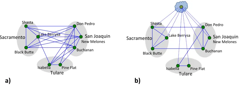
2.1 Graphical structure between a collection of 8 reservoirs without latent variables (a) and with latent variables (b). Green nodes represent reservoirs (variables) and the clouded green node represents latent variables. Solid blue lines represent edges between reservoirs and dotted edges between reservoirs and latent variables. The reservoirs have been grouped according to hydrological zones. . . 11 2.2 (a): Q-Q plot of the entire set of 55 reservoirs. (b): Q-Q plot

of 54 reservoirs (excluding the Farmington reservoir). The Q-Q plots are against a multivariate Gaussian distribution. Notice that y = x is a close approximation to the Q-Q plot implying that 54 reservoirs (excluding Farmington reservoir) are well approximated by a multivariate Gaussian distribution. . . 13 2.3 Training and validation performance of graphical modeling for

dif-ferent values of the regularization parameter λ. The training per-formance is computed as the average log-likelihood of training sam-ples and the validation performance is computed as the average log-likelihood of validation samples. . . 18 2.4 Sensitivity of the graphical model estimate to perturbations of λ

around the optimal valueλ= 0.23 (this choice ofλleads to optimal validation performance): we observe that strong edges in the original model are strong edges in the perturbed model (i.e., with perturbed

λ) with approximately the same strength. . . 18 2.5 Linkages between reservoir pairs in the graphical model (upper

(12)

2.6 A schematic of California and its river network with some reservoir connections. Green nodes represent the 5 pairs of reservoirs with strongest edge strength in the graphical model. The red nodes rep-resent the five strongest edges to Folsom Lake, which is the most connected reservoir in the network. The acronyms for the reservoirs are: WRS (Wishon), COY (Coyote Valley), INV (Indian Valley), BER (Lake Berryessa), SHA (Shasta), BUL (Bullards Bar), FOL (Folsom Lake), CMN (Camanche), DNP (Don Pedro), EXC (New Exchequer), ALM (Almanor Lake), DAV (Lake Davis), SWB (Main Strawberry), RLF (Relief), CHV (Cherry Valley), and HTH (Hetch-Hetchy). . . 21 2.7 a) Ratios of drainage areas between pairs of reservoirs connected

with an edge and their corresponding edge strengths in a graphical model. b) Ratios of elevations of pairs of reservoirs connected with an edge and their corresponding edge strengths in a graphical model. c) Ratios of drainage areas between pairs of reservoirs connected with an edge and their corresponding edge strengths in an unregularized maximum likelihood (ML) estimate. d) Ratios of elevations of pairs of reservoirs connected with an edge and their corresponding edge strengths in an unregularized maximum likelihood (ML) estimate. . . 22 2.8 Linkages between reservoir pairs in the latent-variable sparse

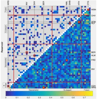
graph-ical model (upper triangle) with varying number of latent variables compared with those of the ordinary sparse graphical model model (lower triangle). Connection strength s(r,r0)is shown in the image map, with unlinked reservoir pairs drawn in gray. The four hydro-logical zones are separated by red lines. Red boxes surround the five strongest connections in each model. . . 26 2.9 System-wide response to drought in a conditional latent variable

(13)

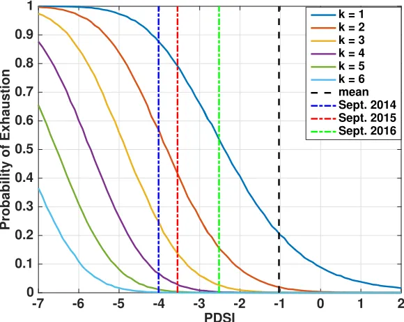
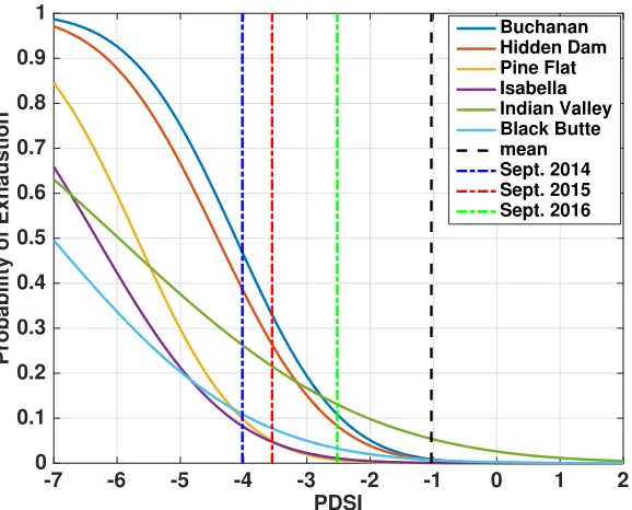
2.10 Individual reservoir responses to drought in a conditional latent vari-able graphical model: probability that six most-at-risk reservoirs out of 31 large reservoirs (with capacity≥ 108m3) will have volume drop below zero; Dashed black line: average September PDSI (September 2004-September 2015). Dashed blue line: September 2014 PDSI. Dashed red line: September 2015 PDSI. Dashed green line: Septem-ber 2016 PDSI. . . 35 2.11 Inflows, outflows, precipitation, and water levels for the Buchanan

and Hidden Dam reservoirs during the extreme drought period of 2014-2015. Notice that there was little precipitation, leading to marginal inflow of water into each reservoirs. Due to heavy man-agement, there was little to no outflow of water from these reser-voirs, preventing them from running dry. These figures are obtained from the Sacramento District Water Control Data System at http: //www.spk-wc.usace.army.mil/plots/california.html. . . 36 2.12 PDSI vs reservoir levels for the Buchanan and Hidden Dam reservoirs

during the period of study (i.e. January 2003 to November 2016). Notice a positive correlation between PDSI and the reservoir volumes: smaller values of PDSI generally lead to lower reservoir volumes. During the 2014-2015 drought period (shown in red), the correlation is substantially reduced as a result of stringent management efforts. . 37 3.1 The quantities_EhtraceP_T_ˆ_(D)P_T?⊥

i

(in blue) and_Etrace P_avgP_T?⊥

(in red) as a function ofλfor SNR = 1.6 (right) and SNR = 0.8 (left) in the synthetic matrix completion setup. The cross-validated choice of λis shown as the dotted black line. Here ‘N-S’ denotes no sub-sampling and ‘W-S ’ denotes with subsub-sampling. . . 51 3.2 Relationship betweenrs3andαin Algorithm 1 for a large range ofλ

and SNR= {0.4,0.8,1.2,50}. . . 63 3.3 False discovery of subspace stability selection vs a non-subsampled

approach with SNR = 1.6,0.8. Here, we choose a rank-3 approxi-mation of the non-subsampled approach and rS3 = 3 in Algorithm

(14)

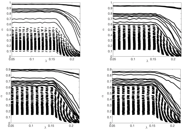
3.4 top left: γ = 30 ; rank sel. = 6 and k[P_T_ˆ_(D(_n_/₂₎₎,P_T?⊥]k_F ≈ 41 ;top right: γ =20 ; rank sel.=6 andk[P_T_ˆ_(D(_n_/₂₎₎,P_T?⊥]k_F ≈91 ; bottom

left: γ =30 ; rank sel.= 10 andk[P_T_ˆ_(D(_n_/₂₎₎,P_T?⊥]k_F ≈ 69 ; bottom right: γ = 30 ; rank sel. = 10 and k[P_T_ˆ_(D(_n_/₂₎₎,P_T?⊥]k_F ≈ 114. False discovery of subspace stability selection as a function ofαfor matrix denoising setting. The blue curve is false discovery obtained by subspace stability selection; the red curve is Theorem 4 bound; the yellow curve is average dimension of the selected tangent space; and the dotted line is false discovery from using entire data. Subspace stability selection has small but nonzero false discoveries. As an example, for γ = 20, rank selected = 6, and α = 0.9, subspace stability selection chooses on average a rank-3 model with 11.7 false discoveries. Here dim(T?⊥)=37636. . . 69 3.5 False discovery vs power with (a) matrix completion and (b) linear

measurements over 20 different problem instances (varying rank and noise level). Blue crosses corresponds to the performance of the non-subsampled approach and red crosses correspond to subspace stability selection with α = 0.7. For the instances where standard deviation divided by mean is greater than 0.01, we show one sigma rectangle around the mean. The lines connect dots corresponding to the same problem instance. Both the false discovery and the power are normalized by dividing the expressions (3.3) and (3.4) by dim(T?⊥)

and dim(T?), respectively. . . 71 3.6 Collaborative filtering: MSE on holdout set of non-subsampled

ap-proach (denoted ‘N-S’ and colored in blue) and subspace stability se-lection (denoted ‘S3’ and colored in red). Dotted black line represents the cross-validated choice ofλwith the non-subsampled approach. . 72 3.7 Urban hyperspectral image (left) and spectra of three materials present

in the image (right). The data and the population spectra are obtained fromhttp://www.escience.cn/people/feiyunZHU/Dataset_ GT.html. . . 73 4.1 left: structure and rank consistency of Poisson (observed) and Bernoulli

(15)

4.2 (left) Graphical model without latent variables having 5% sparsity and (right) graphical model with rank 4 and 2% sparsity. Here senators are clustered together according to their party affiliation with Democrats labeled by blue bracket and Republicans by red bracket. . . 89 4.3 The graphical model with latent variables underlying 40 miRNA. The

strongest edge is between miR-1288 and miR-2110. . . 90 5.1 Imaging spectroscopy data collection: instrument with multiple

sen-sors hovering over space in a flight line collecting spectral profile for each pixel location. . . 94 5.2 left: Snapshot of a scene from the ‘ang20150420t160719’ flight;

right: spectral refractivity co efficient of methane gas across infrared and visible spectrum. . . 104 5.3 Dependency structure of the factorizable precision approach (5.10).

Notice a strong correlation across multiple pixels away. . . 104 5.4 left: matched-filter outputs of our modeling approach (5.10) and i.i.d

approach on the test dataset; right: matched-filter outputs of our modeling approach (5.10) and i.i.d approach on the training dataset. . 106 6.1 Synthetic data: plot shows the error (defined in the main text) and

probability of correct structure recovery in composite factor models. The four models studied are(i) (k_x,ku)= (1,1),(ii) (k_x,ku)=(2,2), and (iii) (k_x,ku) = (3,3), and (iv) (k_x,ku) = (4,4). For each

plot-ted point in (b), the probability of structurally correct estimation is obtained over 10 trials. . . 128 6.2 Number of latent factors vs. average log-likelihood over testing set.

These results are obtained by sweeping over parameters ˜λn ∈ [0.04,4]

in increments of 0.004 and solving the convex program (6.18). . . 129 A.1 Variation in false discoveryEtrace PTS3(α)PT?⊥ and powerE

(16)

LIST OF TABLES

Number Page

2.1 Training and validation performances of unregularized maximum likelihood (ML) estimate, independent reservoir model, and graphical model. As larger values of log-likelihood are indicative of better performance, the graphical model is the superior model. . . 17 2.2 Covariates and correlations with the latent space before and after

removing PDSI . . . 30 3.1 False discovery of subspace stability selection vs a non-subsampled

approach on the stylized matrix completion problem. The maximum possible amount of false discovery is dim(T?⊥)=(70−10)2= 3600. 64 3.2 False discovery of subspace stability selection vs a non-subsampled

approach with SNR=0.8 and rank of the estimate set to vary from 1 to 5. The maximum possible amount of false discovery is dim(T?⊥)=

3600. . . 66 4.1 Finding the largest principal angle between the estimated latent space

(e.g. col-space(B?)) and the population latent space (e.g. col-space(Lˆ)) for the Poisson-Bernoulli cycle with different number of latent vari-ables and number of observations. . . 86 4.2 Comparing the FD and PW of the column-space estimate obtained

from employing a nuclear norm vs a tailored regularizer that exploits the structure of the latent variables. . . 87 5.1 Training and validation performances of i.i.d. model employed in

[Tho+15] and our proposed model (5.10). . . 105 6.1 Ranges of γ and the corresponding values of α and β that satisfy

Assumptions 1,2, and 3. . . 124 6.2 Number of composite factor models with rank(Θˆyx) = 1, . . . ,5 that

satisfy the requirements of step 2 in Algorithm 1(for the factor model with 10 latent variables). . . 130 6.3 Deviation of the candidate composite factor model from the factor

model consisting of 10 latent variables. . . 130 6.4 Strength of each covariate in the composite factor model with

(17)

C h a p t e r 1

INTRODUCTION

An overarching challenge in science and engineering is to develop concise and interpretable frameworks that characterize the relationships among a large collec-tion of variables. As an example, in computacollec-tional biology, a common scientific discovery involving a gene regulatory network is to determine how variation in one gene impacts the others genes in the network. In water resources, a complete understanding of the relationship among the different water entities in a network provides an important tool to enforce effective and sustainable policies. Finally, in imaging spectroscopy, characterizing the relationship among the spectral profile of patches in a scene is crucial for the accuracy of existing detection techniques (e.g., matched filters). A significant difficulty that arises with finding the statis-tical dependencies among a collection of variables is that we do not have sample observations of some of the relevant variables. These latent (hidden) variables complicate finding a concise representation, as they introduce confounding depen-dencies among the variables of interest. Consequently, significant efforts over many decades have been directed towards the problem of accounting for the effects of latent phenomena in statistical modeling via latent-variable techniques. Commonly employed latent-variable models include factor analysis, latent dirichlet allocation, mixture distributions, latent-variable graphical models, etc.

(18)

1.1 Motivating Application

An application that has motivated many of the methodological advances made in this thesis is the California reservoir network. The reservoir network, consisting of 1530 reservoirs, is California’s major defense against severe droughts, which is frequently experienced in the state. For four years, from 2012 to 2015, California was in a state of severe drought on par with the worst periods in the past 1,200 years [Agh+14]. The impact of the drought was exacerbated by a fundamental limitation in our ability to predict water levels in reservoirs. Which reservoir will dry up first? What is the likelihood of systemic failure (i.e. multiple large reservoirs exhausting)? Answering these sorts of questions would enable policy makers and water managers to mitigate the damage caused to California’s 40 million residents.

Previous analysis has focused on the behaviour of a small collection of reservoirs using physical laws or via empirical techniques. Due to the size and complexity of the reservoir networks, these approaches have been difficult to carry out. Specifically, a challenge that must be overcome is to understand the influence of external factors on the reservoirs, as well as reservoir interdependencies, since one reservoir failing can negatively affect other reservoirs in the network. The external factors that strongly affect reservoirs may be measurable phenomena (e.g. precipitation and temperature), or hard-to-quantify influence of human operator. In other words, the external factors may be unobserved or latent. To that end, in Chapter 2, we employ a class of latent variable models, known as latent-variable graphical modeling, where the graph connections encode reservoir dependencies and the latent variables account for the external factors. All of these components are learned from data and are utilized to characterize the system-wide response of reservoirs. With this model in hand, we obtain a clearer picture of the demands placed on reservoirs during drought, and propose a practical guideline for policies that can lead to more sustainable water resources. The results of Chapter 2 correspond to the paper [Tae+17].

(19)

known as cross-validation, which does not offer any theoretical guarantees. Next, many latent-variable approaches assume that the variables of interest are Gaussian to produce computationally appealing and statistically accurate procedures. With reservoirs, we overcome this limitation by averaging daily observations to obtain monthly volumes, and validate that the Gaussianity assumption is reasonable after this preprocessing. Furthermore, latent-variable modeling techniques often assume that all observations are identically and independently distributed. With reservoirs, we removed seasonality and verified that the dependencies between observations is substantially reduced. Finally, latent variables produced from data are typically mathematical objects that without semantics. In the reservoir work, we employ a simple post-hoc correlation analysis to link potentially relevant auxiliary variables to learned latent variables to find matches.

1.2 Methodological Contributions

Motivated by these limitations, this thesis provides the following methodologi-cal contributions: an inference procedure to ensure that the model draws accurate inferences about some underlying phenomena, a convex optimization technique to identify a latent-variable graphical model for non-Gaussian variables, a math-ematically rigorous and computationally efficient approach to handle non-iid and high-dimensional data, and finally, a convex optimization procedure to provide semantics to latent-variables. Throughout this thesis, we will explore how these methodologies will not only benefit reservoir modeling, but also applications in hyperspectral imaging, social networks, and collaborative filtering.

Below, we provide more details of the contributions of this thesis beyond the reservoir analysis. Details about related previous work are given in the relevant chapters. The research and results of Chapters 3 and 6 correspond to completed papers [TSC19] and [TC18], respectively. The work in Chapters 4 and 5 correspond to papers that are in preparation.

Chapter 3 - Inference in Low-rank Estimation Low-rank models are ubiquitous

(20)

represent the direction of moving targets. Given the importance of row/column space structures, how do we evaluate the extent to which our model has learned true or false discoveries about the relevant phenomena?

A common approach to statistical model selection – particularly in scientific domains in which it is of interest to draw inferences about an underlying phenomenon – is to develop powerful procedures that provide control onfalse discoveries. Such methods are widely used in inferential settings involving variable selection, graph estimation, and others in which a discovery is naturally regarded as a discrete concept. However, this view of a discovery is ill-suited to many model selection and structured estimation problems in which the underlying decision space is not discrete. We describe a geometric reformulation of the notion of a discovery, which enables the development of model selection methodology for a broader class of problems. We highlight the utility of this viewpoint in problems involving subspace selection and low-rank estimation, with a specific algorithm to control for false discoveries in these settings. Concepts from algebraic geometry (e.g. tangent spaces to determinantal varieties) play a central role in the proposed framework.

Chapter 4 - Latent Variable Graphical Modeling: Beyond Gaussianity The

algorithm to fit a latent-variable graphical model to reservoir volumes in Chapter 2 is appropriate when the variables are Gaussian. In many scientific and engineer-ing applications, the set of variables one wishes to model strongly deviate from Gaussianity. Existing techniques to fit a graphical model to data suffer from one or more of these deficiencies: a) they are unable to handle non-Gaussianity, b) they are based on non-convex or computationally intractable algorithms, and c) they cannot account for latent variables. We develop a framework, based on Generalized Linear Models, that addresses all these shortcomings and can be efficiently optimized to obtain provably accurate estimates. A particularly novel aspect of our formulation is that it incorporates regularizers that are tailored to the type of latent variables: nuclear norm for Gaussian latent variables, max-2 norm for Bernoulli variables, and complete positive norm for Exponential variables. For each case, we provide a semidefinite relaxation and demonstrate that the associated norm yields a better sample complexity (than the nuclear norm) for similar computational cost. We fur-ther demonstrate the utility of our approach with data involving U.S. Senate voting record.

Chapter 5 - Model Selection with non-iid DataThe data we observe and process

(21)

Chapter 2 exhibit significant temporal correlations so that the data is non-iid, and the reservoir network is large so that the data is high-dimensional. Existing techniques that model such complex datasets require O(n2p6) computations (n : number of observations, p: number of variables), which is a significant bottleneck for large

n; p. By appealing to ideas from Stochastic Partial Differential Equations (SPDE) and covariance selection, we provide a framework that blends temporal/spatial and network modeling inO(np2+nlog(n)p+p6)computations. Using this methodology, we are able to efficiently obtain high-dimensional models with rich dependencies across observations. We apply our approach to signature detection in hyperspectral imaging and demonstrate improved performance over existing techniques.

Chapter 6 - Interpreting Latent Variables Via Convex OptimizationFactor

(22)

C h a p t e r 2

LATENT VARIABLE GRAPHICAL MODELING WITH

APPLICATION TO RESERVOIR MODELING

As described in Chapter 1, many of the research questions that are tackled in this thesis stem from an application involving the statistical modeling of the California reservoirs. In this chapter, we will dive deep into this application, discuss the chal-lenges that arise from modeling a system of reservoirs, and propose latent-variable methodologies that address these challenges. The results of this chapter are pub-lished in [Tae+17] and were developed jointly with John Reager, Michael Turmon and Venkat Chandrasekaran. The author contributed by performing data prepro-cessing, developing modeling framework & algorithms to analyze the data, and implementing the numerical methods to produce the final results. The description of the work contained in this chapter was written by the author.

2.1 Introduction

Motivation

The state of California depends on a complex water management system to meet wide-ranging water demands across a large, hydrologically diverse domain. As part of this infrastructure, California has constructed 1530 reservoirs having a collective storage capacity equivalent to a year of mean runoff from California rivers [Gra99]. The purpose of this system is to create water storage capacity and extend seasonal water availability to meet agricultural, residential, industrial, power generation, and recreational needs.

(23)

multiple large reservoirs.

Such an analysis has been difficult to carry out on a system-wide scale due to the size and complexity of the reservoir network. In one direction, a body of work has focused on characterizing the behavior of a small collection of reservoirs using physical laws (e.g. [CL04; Chr+06; NW15]). Such approaches quickly become intractable in settings with large numbers of reservoirs whose complex management is based on multiple economic and sectoral objectives [How+14]. The hard-to-quantify influence of human operators and the lack of system closure have made the modeling and prediction of reservoir network behavior using physical equations challenging in hydrology and climate models [Sol+16]. In a different direction, numerous works have developed empirical techniques for modeling the behavior of a small number of reservoirs (e.g. [RW83; Pha89; NG91; NG93; BHH03; HE07; BP08; Wis+10; Che+15]). However, these methods are not directly applicable to modeling a large reservoir network, as the water levels of major reservoirs in California exhibit complex interactions and are statistically correlated with one another (as is demonstrated by our analysis). This necessitates a proper quantification of the complex dependencies among reservoirs in determining the systemic characteristics of the reservoir network.

The focus of this work is to develop a statewide model over the California reservoir network that addresses the following scientific questions:

1. What are the interactions or dependencies among reservoir holdings? In particular, how correlated are major reservoirs in the system?

2. Are there common external factors influencing the network globally? Could these external drivers cause a system-wide catastrophe?

(24)

Answering these questions for the California reservoir system raises a number of challenges, and it is important that any modeling framework that we consider addresses these challenges. First, reservoirs with similar hydrological attributes (e.g. altitude, drainage area, spatial location) tend to behave similarly. As an example, a pair of reservoirs that is approximately at the same altitude or in the same hydrological zone are more likely to have a stronger correlation than those in different altitudes / zones. Therefore, we seek a framework that ably models the complex heterogeneities in the reservoir system. A second challenge, which is in some sense in competition with the first one, is that compactly specified models are much more preferable to less succinct models, as concisely described models are often more interpretable and avoid problems associated with over-fitting. Finally, it is crucial that models with both of the preceding attributes have the additional feature that they can be identified in a computationally efficient manner.

Approach and Results

(25)

hydrological zone) after conditioning on volumes of reservoirs in the central portion of the state (e.g. Black Butte, Lake Berrysa, New Melones, Buchanan, and Don Pedro). These relationships are encoded in a graphical model of Figure 1(a). In particular, note that Shasta has an edge linking it to each of the reservoirs {Black Butte, Lake Berrysa, Don Pedro, New Melones, Buchanan}, but does not have an edge connecting it to the reservoirs {Pine Flat, Isabella}. Figure 1(a) is, of course, a cartoon demonstration of a graphical modeling framework. In practice, identifying conditional dependencies between pairs of reservoirs in large networks such as the one considered in our work is a challenging problem, and we describe tractable approaches to learning such a graphical structure underlying the complex California reservoir system in a completely data-driven manner in Section 3. To the best of our knoweledge, this is the first work that applies graphical modeling techniques to model reservoirs or other water resources.

The graphical modeling framework provides a common lens for viewing two frequently employed statistical techniques. On the one hand, a classical approach for obtaining a multivariate Gaussian distribution over reservoir volumes is via a maximum likelihood estimator. This estimator has been widely used in various do-mains in the geophysical sciences for multivariate analysis of a collection of random variables [Wac03]. The model obtained by this maximum likelihood estimator is specified by a completely connected graphical structure, where all reservoirs are conditionally correlated given all other reservoirs. On the other hand, an indepen-dent reservoir model analyzes the behavior of an individual reservoir indepenindepen-dently of the other reservoirs in the network. This model results in a fully disconnected graphical model. In this chapter, we learn a statistical graphical model over the reservoir network in a data-driven manner based on historical reservoir data. This model yields a sparse (yet connected) graphical structure describing the network interactions. We demonstrate that this model outperforms the model obtained via classical maximum likelihood estimator and an independent reservoir model. Thus, the reservoir behaviors are not independent of one another but can be specified with a moderate number of interactions. We demonstrate that a majority of these interactions are between reservoirs that are in the same basin or hydrological zone, and among reservoirs that have similar altitude and drainage area.

(26)

collection of nearby reservoirs might be influenced by a common snowpack variable. Without observing this common variable, all reservoirs in this set would appear to have mutual links, whereas if snowpack is included in the analysis, the common behavior is explained by a link to the snowpack variable. Accounting for latent structure removes these confounding dependencies and leads tosparser and more localizedinteractions between reservoirs. Figure 2.1(b) illustrates this point. Latent variable graphical modeling offers a principled approach to quantify the effects of external phenomenathat influence the entire reservoir network. In particular, this modeling framework uses observational data to (a) identify the number of global drivers (e.g. latent variables) that summarize the effect of external phenomena on the reservoir network, and (b) identify the residual reservoir dependencies after accounting for these global drivers. Our experimental results demonstrate that the reservoir network at a monthly resolution has two distinct global drivers, and residual dependencies persist after accounting for these global variables.

Latent variable graphical modeling obtains a mathematical representation of the global drivers of the reservoir network. One is naturally interested in linking these mathematical objects to real world signals (e.g. statewide Palmer Drought Severity Index, snowpack, consumer price index). We present an approach for associating semantics to these global drivers. We find that the statewide Palmer Drought Severity Index (PDSI) is highly correlated (ρ≈ 0.88) with one of the global drivers. PDSI is then included as a covariate in thenextiteration of the graphical modeling procedure to learn a joint model over reservoirs and PDSI. Using this model, we characterize the system-wide behavior of the network to hypothetical drought conditions. In particular, we find that as PDSI approaches −5, there is a probability greater than 50% of simultaneous exhaustion of multiple large reservoirs. We further present an approach for identifying specific reservoirs in the network that are at high risk of exhaustion during extreme drought conditions. We find that the Buchanan and Hidden Dam reservoirs are at high risk and describe water management policies and practices that were enforced to prevent exhaustion.

2.2 Dataset and Model Validation

(27)

Tulare Shasta

Black Bu/e

Lake Berrysa

Isabella Pine Flat Don Pedro

New Melones Buchanan

San Joaquin

Sacramento _Sacramento

Tulare Shasta

Black Bu/e

Lake Berrysa

Isabella Pine Flat Don Pedro

Buchanan New Melones

a) b)

[image:27.612.110.527.74.222.2]

San Joaquin

Figure 2.1: Graphical structure between a collection of 8 reservoirs without la-tent variables (a) and with latent variables (b). Green nodes represent reservoirs (variables) and the clouded green node represents latent variables. Solid blue lines represent edges between reservoirs and dotted edges between reservoirs and latent variables. The reservoirs have been grouped according to hydrological zones.

Reservoir Time Series&Preprocessing Techniques

As described in Section 1, there are 1,530 reservoirs in California. In this work, we perform statistical analysis on the largest 60 reservoirs in California. We apply our analysis to a subset of the reservoirs, as they have a large amount of historical data available. Our technique can be extended to a larger collection of reservoirs given sufficient data. For these 60 reservoirs, daily volume data is available during the period of study (January 2003 — November 2016). We excluded five reservoirs with more than half of their values undefined or zero, leaving 55 reservoirs. This list of daily values was inspected using a simple continuity criterion and approximately 50 specific values were removed or corrected. Corrections were possible in six cases because values had misplaced decimal points, but all other detected errors were set to missing values. The most common error modes were missing values that were recorded as zero volume, and a burst of errors in the Lyons reservoir during late October 2014 that seems due to a change in recording method at that time.

The final set of 55 reservoir volume time series spans 5083 days over the 167 months in the study period. It contains two full cycles of California drought (roughly, 2007 — 2008 and 2012 — 2015) and three cycles of wet period (2004 — 2006, 2009 — 2011, 2016). Four California hydrological zones are represented, with 25, 20, 6, and 4 reservoirs in the Sacramento, San Joaquin, Tulare, and North Coast zones, respectively.

(28)

vol-umes at a monthly time scale. In particular, we average the data from daily down to 167 monthly observations. The reservoir data exhibit strong seasonal components. As such, a seasonal adjustment step is performed to remove these predictable pat-terns, so that we can model deviations from the underlying trend in the reservoir be-havior. Specifically the steps are as follows Let{y¯(i)}ntrain

i=1 ⊂ R

55_and_{_y_¯(i)_}ntest

i=1 ⊂ R 55

be the averaged monthly reservoir volumes in the training and validation set respec-tively. Focusing on a reservoirr and the month of January, let µy¯r be the average

reservoir level during January (obtained only from training observations). For each observationi in January, we apply the transformation: ˜y_r(i) = y¯_r(i)− µy¯r. We repeat

the same steps for all months. Furthermore, lettingσr be the sample standard devi-ation of the training observdevi-ations{y˜_r(i)}ntrain

i=1 , we produce unit variance observations

with the transformation,y_r(i) = 1 σr1/2

˜

y_r(i). Before being used in the fitting algorithms, each time series is also rescaled by its standard deviation so that each series has unit variance. We note that our statistical approach identifies correlations between reservoir volumes. Since correlation between two random variables is normalized by their respective variances, this transformation is appropriate. We repeat the same steps for all reservoirs to obtain the preprocessed reservoir observations {y(i)}ntrain

i=1

and{y(i)}ntest

i=1.

With the exception of the Farmington reservoir (which has volume less than 108 m3), the joint volume anomalies of the remaining 54 reservoirs (after prepro-cessing) are well-approximated by a multivariate Gaussian distribution. This is demonstrated by a Q-Q plot in Figure 2.2. Since a large amount of historical data is available for the Farmington reservoir, we have included it in our analysis. These observed properties suggest that the reservoir data is amenable to the multivariate Gaussian models we employ in this chapter.

Covariate Time Series

(29)

0 10 20 30 40 50 60 70 80 Chi-square quantile

0 20 40 60 80 100

Squared Mahalanobis distance

Q-Q plot y = x

30 40 50 60 70 80 90

Chi-square quantile 0

10 20 30 40 50 60 70 80

Squared Mahalanobis distance

[image:29.612.112.504.61.227.2]

Q-Q plot y = x

Figure 2.2: (a): Q-Q plot of the entire set of 55 reservoirs. (b): Q-Q plot of 54 reservoirs (excluding the Farmington reservoir). The Q-Q plots are against a multivariate Gaussian distribution. Notice that y = x is a close approximation to the Q-Q plot implying that 54 reservoirs (excluding Farmington reservoir) are well approximated by a multivariate Gaussian distribution.

Sierra Nevada snow pack covariate (manually averaged in the Sierra Nevada region where the elevation is over 100 m, gridded observations downloaded from NOAA). Note that since we are interested in statewide covariates that exert influence over the entire network, these hydrological indicators were averaged over the state of California (or in the case of snowpack and Colorado river discharge, averaged over a large region in the Sierra Nevada and Colorado river respectively). In addition to these hydrological indicators, we use the following economic factors: statewide number of agricultural workers (downloaded from State of California Employment Development Department) and statewide consumer price index (downloaded from Department of Industrial Relations).

For each of the 7 covariates, we obtain averaged monthly observations from 2003—2016. We apply a time lag of two months to the covariates temperature, snowpack, Colorado river discharge, and Palmer Drought Severity Index (the rea-son for a two months lag is explained in Section 4.4). As with the reservoir time series, we remove seasonal patterns with a per-month average, and rescale to obtain unit variance variables.

Model Validation

(30)

[HTF09]. The objective of this technique is to produce models that are not overly tuned to the idiosyncrasies of observational reservoir data, so that these models are representative of future reservoir behavior. In a holdout validation framework, the available data is partitioned into a training set, and a disjoint validation set. The training set is used as input to a fitting algorithm to identify a model. The accu-racy of this model is then validated by computing the average log-likelihood of the validation set with respect to the distribution specified by the model. Here, larger values of log-likelihood are indicative of better fit to data. For our experiments, we set aside monthly observations of reservoir volumes and covariates from January 2004 — December 2013 as a training set (ntrain = 120) and monthly observations

from January 2003 — December 2003 and January 2014 — November 2016 as a (disjoint) validation set (ntest = 47). Both the training and validation observations

contain a signficiant amount of annual and inter-annual variability.

2.3 Dependencies Underlying the Reservoir Network

Method: Graphical Modeling

A common approach for fitting a graphical model to reservoirs is to choose the simplest model, that is, the sparsest network that adequately explains the observa-tional data. Easing this taks, for Gaussian graphical models, the graphical structure is encoded in the sparsity pattern of the precision matrix (inverse covariance ma-trix) over the variables. Specifically, zeros in the precision matrix of a multivariate Gaussian distribution indicate absent edges in the corresponding graphical model. Thus, the number of edges in the graphical model equals the number of nonzeros of the precision matrixΘ. As an example, consider the toy graphical model in Figure 1(a). Suppose that the precision matrixΘof size 8×8 is indexed according to the ordering {Shasta, Black Butte, Lake Beryssa, Isabella, Pine Flat, Don Pedro, New Melones, and Buchanan}. ThenΘhas the following structure:

Θ=

©

«

? ? ? 0 0 ? ? ?

? ? ? ? 0 ? ? ?

0 0 ? ? ? ? ? ?

0 0 0 ? ? ? 0 ?

? ? ? ? ? ? ? ?

? ? ? ? 0 ? ? ?

? ? ? ? ? ? ? ?

ª ® ® ® ® ® ® ® ® ® ® ® ® ® ® ®

¬

(31)

where ?denotes a nonzero value. The intimate connection between a graphical structure and the precision matrix implies that fitting a sparse Gaussian graphical model to reservoir observational data is equivalent to estimating a sparse precision matrix Θ. Thus, the reservoirs are modeled according to the distribution y ∼ N(0, Θ−1), whereΘis sparse. Note that the preprocessing to remove climatology causes the mean to be zero. A natural technique to fit such a model to observational data is to minimize the negative log-likelihood (e.g. maximum likelihood estimation) of data while controlling the sparsity level of Θ. The log-likelihood function of the training observations D_train = {y(i)}ntrain

i=1 ⊂ R

55 _{(after removing some additive}

constants and scaling) is given by the concave function

`(Θ;D_train)=log det(Θ) −tr[Θ·Σ_n] , (2.1) where Σ_n = _n1

train Íntrain

i=1 y

(i)

y(i)0 is the sample covariance matrix. Thus, fitting a graphical model toD_traintranslates to searching over the space of precision matrices to identify a matrix Θthat is sparse and also yields a small value of−`(Θ;D_train). This formulation, however, is a computationally intractable combinatorial problem. Recent work [YL07; FHT08] has identified a way around this road block by using a convex relaxation:

ˆ

Θ=arg min Θ∈_S55

−`(Θ;D_train)+λ kΘk₁

s.t. Θ 0 . (2.2)

The notation _S55 denotes the set of symmetric 55× 55 matrices. The constraint

0 imposes positive definiteness so that the joint distribution of reservoirs is non-degenerate. The regularization term k · k₁denotes the L1norm (element-wise sum

of absolute values) that promotes sparsity in the matrix Θ. The L1 penalty, and

more broadly, regularization techniques, are widely employed in inverse problems in data analysis to overcome ill-posedness and avoid problems such asover-fitting to moderate sample size (see the textbooks/monographs [BG11; Wai14] and the references therein). These regularization approaches have proved to be valuable in many applications, including cameras [Dua+08], magnetic resonance imaging [Lus+08], gene regularity networks [ZK14], and radar [HS09].

(32)

Generally,Σ−_n1will not contain any zeros. This implies that the estimated graphical structure is fully connected with close fit to the training data D_train. However, as explored in Section 3.2, this model may be over-tuned to the idiosyncrasies of the training observationsD_trainand will not generalize to future behavior of reservoirs (a phenomenon known asover-fitting). Larger values ofλyield a sparser graphical model with very large λ resulting in a completely disconnected graphical model where the reservoirs are independent of one another. Importantly, for any choice of λ > 0, (2.2) is a convex program with a unique optimum, and can be solved efficiently using general purpose off-the-shelf solvers [TTT16]. Further theoretical support of this estimator is presented in [Rav+11b].

We select the regularization parameterλbyholdout validation. In particular, for any choice ofλ, we supply the training observationsD_trainto (2.2) to learn a graphical model and compute the average log-likelihood of this model on the validation set

D_test = {y(i)}ntest

i=1 ⊂ R

55_{. We sweep over all values of} _λ_{to choose the model with}

the best validation performance. Let the selected model (after holdout validation) be specified by the precision matrix ˆΘ. As discussed earlier, the matrix ˆΘspecifies the structural properties of the graphical model of the network. An edge between reservoirsr andr0is present in the graph if and only if ˆΘ_r_,_r0 _, 0, with larger

mag-nitudes indicating stronger interactions. We denote the strength of an edge as the normalized magnitude of the precision matrix entry, that is,

s(r,r0)= |Θˆ_r_,_r0|(Θˆ_r_,_rΘˆ_r0_,_r0)1/2 ≥ 0. (2.3)

The quantitys(r,r0)can be viewed as the partial correlation between reservoirsrand

r0

, given all other reservoirs. In particular, a larges(r,r0)indicates that reservoirsr andr0are highly correlated even after accounting for the influence of all the other reservoirs in the network. A small value of s(r,r0) indicates that the reservoirs r andr0are weakly correlated conditioned on all the reservoirs. Finally, s(r,r0) = 0 indicates that reservoirsr andr0 are independent conditioned on all the remaining reservoirs.

Results: Graphical Model of Reservoir Network

(33)

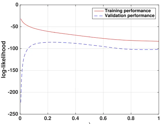
observationD_trainand the validation performance as the log-likelihood of validation observationsD_test. Figure 2.3 illustrates the training and validation performances for different values ofλ. Recall thatλ =0 corresponds to an unregularized maximum likelihood estimate and λ = 1 corresponds to independent reservoir model. We choseλ = 0.23 to obtain a graphical model with the best validation performance. Results of Figure 2.3 demonstrate that the training performance is a decreasing function ofλ: smaller values ofλlead to a closer fit to training observations. How-ever, small values ofλyield a high complexity model that fits the idiosyncrasies of the training data and thus suffers from over-fitting. This is evident from the poor validation performance of unregularized ML estimate (whenλ=0). The graphical model is the superior model since it has a better validation performance than the unregularized ML estimate and an independent reservoir model. Thus the reservoir behaviors are not independent but can be characterized by a moderate number of dependencies. In the supplementary material, we characterize the sensitivity of the graphical model to the choice of the regularization parameterλ.

Model Training performance Validation performance

unregularized ML estimate (λ=0) −23.91 -1140.4 independent reservoir model (λ= 1) −83.23 −101.95

graphical model (λ=0.23) -63.52 -85.54

Table 2.1: Training and validation performances of unregularized maximum likeli-hood (ML) estimate, independent reservoir model, and graphical model. As larger values of log-likelihood are indicative of better performance, the graphical model is the superior model.

To demonstrate that the graphical model estimate does not vary significantly under small perturbations to λ, we also obtain graphical model estimates withλ = 0.26 andλ=0.20 (Recall that the edge strengths in a graphical model contain the relevant information of the model). Figure 2.4(a) compares the edge strengths of the model withλ= 0.23 and the model withλ= 0.20. Furthermore, Figure 2.4(b) compares the edge strengths of the model with λ = 0.23 and the model with λ = 0.26. Evidently, strong edges persist across all models, with a few weak edges removed or added as λis varied. The total number of edges in the graphical model when

(34)

0 0.2 0.4 0.6 0.8 1

λ

-250 -200 -150 -100 -50 0

log-likelihood

Training performance Validation performance

Figure 2.3: Training and validation performance of graphical modeling for different values of the regularization parameter λ. The training performance is computed as the average log-likelihood of training samples and the validation performance is computed as the average log-likelihood of validation samples.

0 0.05 0.1 0.15 0.2 0.25 0.3 0.35 0.4

Edge Strength (λ = 0.230)

0 0.05 0.1 0.15 0.2 0.25 0.3 0.35 0.4

Edge Strength (

λ

= 0.20)

edge strengths y=x

0 0.05 0.1 0.15 0.2 0.25 0.3 0.35 0.4

Edge Strength (λ_{= 0.23)}

0 0.05 0.1 0.15 0.2 0.25 0.3 0.35 0.4

Edge Strength (

λ

= 0.26)

[image:34.612.166.443.68.282.2]

edge strengths y=x

Figure 2.4: Sensitivity of the graphical model estimate to perturbations ofλaround the optimal valueλ=0.23 (this choice ofλleads to optimal validation performance): we observe that strong edges in the original model are strong edges in the perturbed model (i.e., with perturbedλ) with approximately the same strength.

λ = 0.20, λ = 0.23, andλ = 0.26. These results suggest that our conclusions are not particularly sensitive to the choice of the regularization parameter, although we choseλ=0.23 as it leads to the best validation performance.

(35)

relationships between reservoirs in this graphical model. The five strongest edges in this graphical structure are between reservoirs Relief – Main Strawberry, Cherry – Hetch Hetchy, Invisible Lake – Lake Berryessa, Almanor – Davis, and Coyote Valley – Warm Spring. We show the geographical location of these pairs of reservoirs in Figure . The presence of these strong edges is sensible: each such edge is between reservoirs in the same hydrological zone, and 4 of these 5 edges are between pairs of reservoirs fed by the same river. The five most connected reservoirs in order Folsom Lake, Antelope river, Black Butte River, New Exchequer, and French Meadows, all of which are large reservoirs (volume ≥ 108 m3). We show the five strongest connections to Folsom lake in Figure 2.6 , all of which are either connected or are in close proximity to the Sacramento River. As a point of comparison, the lower triangle of Figure 2.5 shows the graphical structure of the unregularized maximum likelihood estimate. This model yields a fully connected network.

Furthermore, we observe that a majority of interactions in this graphical model are among reservoirs that have similar drainage area (e.g. land where water falls off into reservoirs) and elevation. Figure 2.7 (a) shows a plot of the ratios of drainage areas between pairs of reservoirs connected via an edge and the strength of the connections. Figure 4(b) shows a plot of the ratios of altitudes between pairs of connected reservoirs and the strength of the connections. As a point of comparison, Figures 2.7(c) and 2.7(d) show similar metrics for the unregularized maximum likelihood estimate. Examining Figure 4, we observe that graphical modeling removes (or weakens) dependencies between reservoirs of vastly different drainage area or elevation. This is expected since reservoirs with substantially different drainage area or elevation are less likely to have similar variability.

We observe that a large portion of the strong interactions occur between reservoirs in the same hydrological zone, here denotedh(r). To quantify this observation, we consider

κ=

Í

r,r0_and_h₍_r₎₌_h₍_r0₎s(r,r0)

Í

r,r0s(r,r0)

, (2.4)

(36)

[image:36.612.145.464.71.398.2]

Figure 2.5: Linkages between reservoir pairs in the graphical model (upper triangle) compared with those of the unregularized maximum likelihood estimate (lower triangle). Connection strength s(r,r0) is shown in the image map, with unlinked reservoir pairs drawn in gray. The four hydrological zones are separated by red lines. Red boxes surround the five strongest connections in each model.

We further explore the effect of these external phenomena to remove the confounding relationships between geographically distant reservoirs.

2.4 Global Drivers of the Reservoir Network

(37)

[image:37.612.170.438.156.485.2]

(38)

Confidential manuscript submitted toWater Resource Research

0 500 1000 1500

Drainage Area Ratio 0 0.05 0.1 0.15 0.2 0.25 0.3 0.35 Edge Strength

(a) graphical model

0 10 20 30 40 50 60 70

Elevation Ratio 0 0.05 0.1 0.15 0.2 0.25 0.3 0.35 0.4 Edge Strength

(b) graphical model

0 500 1000 1500

Drainage Area Ratio 0 0.1 0.2 0.3 0.4 0.5 0.6 0.7 0.8 Edge Strength

(c) unregularized ML estimate

0 10 20 30 40 50 60 70

Elevation Ratio 0 0.1 0.2 0.3 0.4 0.5 0.6 0.7 0.8 Edge Strength

[image:38.612.123.492.161.471.2]

(d) unregularized ML estimate

Figure 1. a) Ratios of drainage areas between pairs of reservoirs connected with an edge and their

corre-sponding edge strengths in a graphical model, b) Ratios of elevations of pairs of reservoirs connected with an edge and their corresponding edge strengths in a graphical model, c) Ratios of drainage areas between pairs of reservoirs connected with an edge and their corresponding edge strengths in an unregularized maximum likelihood (ML) estimate, d) Ratios of elevations of pairs of reservoirs connected with an edge and their corresponding edge strengths in an unregularized maximum likelihood (ML) estimate.

6 7 8 9 10 11

A Statistical Graphical Model of the California Reservoir

1

System

2

A. Taeb1_{, J.T. Reager}2_{, M. Turmon}2_{, V. Chandrasekaran}1

3

1_{California Institute of Technology.}

4

2_{Jet Propulsion Laboratory}

5

Corresponding author: Armeen Taeb,[email protected]

–1–

(39)

Method: Latent Variable Graphical Modeling

As shown by [CPW12], fitting a latent variable graphical model corresponds to representing the precision matrix of the reservoir volumes Θ as the difference

Θ = S− L, whereSis sparse, and L is a low rank matrix. The matrixL accounts for the effect of external phenomena, and its rank is equal to the number of global drivers; these global drivers summarize the effect of external phenomena on the reservoir network. The matrix S specifies the residual conditional dependencies among the reservoirs after extracting the influence of global drivers. Moreover, the sparsity pattern ofSencodes the residual graphical structure among reservoirs. As an example, consider the toy model shown in Figure 2.1(b). Suppose that the matrix

Sis indexed according to the ordering {Shasta, Black Butte, Lake Berrysa, Isabella, Pine Flat, Don Pedro, New Melones, and Buchanan}. ThenShas the structure:

S=

©

«

? ? ? 0 0 0 0 ?

? ? ? 0 0 ? 0 0

0 0 0 ? ? 0 0 0

0 0 0 ? ? 0 0 ?

0 0 0 ? ? 0 0 0

0 ? 0 0 0 ? ? ?

0 0 0 0 0 ? ? ?

? 0 0 ? 0 ? ? ?

ª ® ® ® ® ® ® ® ® ® ® ® ® ® ® ®

¬

,

where ? denotes a nonzero entry. Fitting a latent variable graphical model to reservoir volumes is to identify the simplest model, e.g. smallest number of global drivers and sparsest residual network, that adequately explains the data. In other words, we search over the space of precision matrices Θthat can be decomposed as Θ = S − L to identify a matrix S that is sparse, a matrix L that has a small rank, and also yields a small negative log-likelihood −`(D_train,S − L). As with the case of graphical modeling, this formulation is a computationally intractable combinatorial problem. Based on a recent work by [CPW12], a computationally tractable estimator is given by:

(S,ˆ Lˆ)=arg min

S,L∈_S55

−`(S−L;D_train)+λ(kSk₁+γtr(L))

s.t. S− L 0, L 0 . (2.5)

The constraint 0 imposes positive definiteness on the precision matrix estimate

(40)

imposes positive semi-definiteness on the matrixL(see [CPW12] for an explanation of this constraint). Here, ˆL provides an estimate for the low-rank component of the precision matrix (corresponding to the effect of latent variables on reservoir vol-umes), and ˆSprovides an estimate for the sparse component of the precision matrix (corresponding to the residual dependencies between reservoirs after accounting for the latent variables).

The regularization parameter γ provides a trade-off between the graphical model component and the latent component. In particular, for very large values ofγ, the convex program (2.5) produces the same estimates as the graphical model estimator (2.2) (that is, ˆL = 0 so that no latent variables are used). As γ decreases, the number of latent variables increases and correspondingly the number of edges in the residual graphical structure decreases; this is because latent variables account for a global signal common to all reservoirs. The regularization parameterλprovides overall control of the trade-off between the fidelity of the model to the data and the complexity of the model.

As before, the function k · k₁ denotes the L1norm that promotes sparsity in the

matrixS. The role of the trace penalty onLis to promote low-rank structure [Faz02]. As before, forλ, γ ≥ 0, (2.5) is a convex program with a unique optimum that can be solved efficiently. Theoretical support for this estimator is presented in [CPW12].

Similar to the graphical model setting, we use theholdout validationtechnique to determine the number of global latent variables and edges in the graphical structure between reservoirs. Concretely, for a particular choice ofλ, γ, we supplyD_train as input to the program (2.5) to learn a latent variable graphical model and compute the average log-likelihood of this model on the validation setD_test. We sweep over all possible choices ofγ, λand choose a set of parameters that yield the best validation performance.

Let the selected model (after holdout validation) be specified by the parameters

(41)

latent variables as follows: the model estimates the covariance matrix of reservoirs as(Sˆ−Lˆ)−1so thaty ∼ N(0, (Sˆ−Lˆ)−1). Given that the variance of a reservoirris

h

(Sˆ−Lˆ)−1i

r,r, we denote the overall variance of the network as

Í55

r=1

h

(Sˆ−Lˆ)−1i r,r.

The variance of reservoir r, conditioned on k latent variables, is given by(Sˆ−1₎ r.

We thus denote the variance of the network conditioned on k latent variables by Í55

r=1

h ˆ

S−1i

r,r. Furthermore, we define the ratio

δ(k)=

Í55

r=1

h

(Sˆ−Lˆ)−1−Sˆ−1i r,r

Í55

r=1

h

(Sˆ−Lˆ)−1i r,r

(2.6)

as the portion of the variability of the network explained byk latent variables.

Results: Accounting for Drivers of the Reservoir Network

We first explore the effect of global drivers on the connectivity of the reservoir network. Using observations D_train as input to the convex program (2.5), we vary the regularization parameters(λ, γ)to learn a collection of latent variables graphical models. Figure 2.8 shows the residual conditional graphical structure corresponding to each model. We observe that an increase in the number of latent variables leads to sparser structures and stronger inner-zone connections. Indeed, the ratios of inner zone edge strengths to total edge strength are κ = 0.91, κ = 0.91, κ = 0.93,

κ = 0.94, κ = 0.97, and κ = 0.99 for models with 1, 2, 3, 4, 5, and 6 latent variables respectively. These results support the idea that latent variables extract global features that are common to all reservoirs, and incorporating them results in more localized interactions. The residual dependencies that persist (even after including several latent variables) can be attributed to unmodeled local variables.

Further, appealing to relation (2.6), the portion of the variability of the network explained by 1, 2, 3, 4, 5, and 6 latent variables is given byδ(1)= 0.23,δ(2)= 0.25,

δ(3)=0.28,δ(4)= 0.31,δ(5)=0.32, andδ(6)=0.40 respectively. Thus, the effect of latent variables on the network increases as we incorporate more of them in the model. Nonetheless, even 6 latent variables explain less than 50% of the reservoir variability, with the other portion attributed to residual conditional dependencies between reservoirs. Furthermore, this experiment suggests that both the influence of global latent variables and residual dependencies among reservoirs are important factors of the reservoir network variability.

(42)

(a) 1 latent variable (b) 2 latent variables

(c) 3 latent variables (d) 4 latent variables

(e) 5 latent variables (f) 6 latent variables

Figure 1. Linkages between reservoir pairs in the latent-variable sparse graphical model (upper trian-gle) with varying number of latent variables compared with those of the ordinary sparse graphical model model (lower triangle). Connection strengths(r,r0_{) is shown in the image map, with unlinked reservoir pairs}

drawn in gray. The four hydrological zones are separated by red lines. Red boxes surround the five strongest connections in each model.

1

2

3

4

5

[image:42.612.144.461.79.614.2]

–1–

Figure 2.8: Linkages between reservoir pairs in the latent-variable sparse graphical model (upper triangle) with varying number of latent variables compared with those of the ordinary sparse graphical model model (lower triangle). Connection strength

(43)

variable graphical model consisting of two latent variables together with a residual graphical model (conditioned on the latent variables) having 171 edges. This is the model corresponding to Figure 2.8(b). Thus, the reservoir network consists of two global drivers, and some residual dependencies persist after accounting for their influence. The training and validation performance of this model (in terms of log-likelihood) are given by−62.11 and−85.87, respectively.

The conditional dependency relationships between reservoir pairs in this residual graphical structure are shown in the upper triangle of Figure 2.8(b). Comparing this graphical structure with the graphical structure without any latent variables (lower triangle of Figure 2.8(b)), accounting for the global drivers weakens or removes many connections between reservoirs: 134 are removed and 252 are weakened. Of the 134 edges removed, 94 are between reservoirs in different hydrological zones. Further, the latent variable graphical model has comparable model complexity and training/testing performance to the graphical model without latent variables. We conclude that many of the connections in the graphical model (without latent vari-ables) are due to unmodeled global drivers and accounting for these variables leads to fewer remaining conditional dependencies.

Finally, of the 55 reservoirs in our system, 35 are used for sourcing hydroelectric power. In the graphical structure without latent variables, there are 154 pairwise edges between reservoirs that are used for generating hydroelectric power. Once the latent variables are incorporated, all but 15 of these edges are weakened or removed. This suggests that hydroelectric power is strongly correlated to one of the global drivers. We verify this hypothesis in the next section.

Method: Interpreting Latent Variables via Correlation Analysis

Latent-variable graphical modeling identifies a mathematical representation of the global drivers of the reservoir network. Naturally, one is interested in linking these mathematical variables to real-world signals to aid understanding of factors that globally affect the reservoir network. We propose an approach to give physical interpretations to the estimated global drivers. The high level intuition of this approach is to identify a space of all possible latent variable data termedthe latent space. Then we compute the correlation of external covariates (the covariates we consider are in Section 2.2) with this space. Candidate covariates with high correlation are variables that globally influence the reservoir network.