Rochester Institute of Technology
RIT Scholar Works
Theses Thesis/Dissertation Collections
11-1-2008
Detecting relevant changes in high throughput
gene expression data
Anusha Aiyalu Kannan
Follow this and additional works at:http://scholarworks.rit.edu/theses
Recommended Citation
R·I·T
Detecting Relevant Changes in High
Throughput Gene Expression Data
by
Anusha Aiyalu Kannan
A Thesis Submitted in Partial Fulfillment of the Requirements for the Master of Science Degree in Bioinformatics
at the
Rochester Institute of Technology
Department of Biological Sciences College of Sciences
Rochester Institute of Technology Rochester, NY
Approved By:
__________________________________________________________________
Gary R. Skuse, Ph.D Date
Thesis Advisor
__________________________________________________________________
Richard L Doolittle, Ph.D Date
Head, Department of Biological Sciences
_____________________________________________________________________________________
Dr. Robert J. Parody Date
Committee Member
_____________________________________________________________________________________
Anne Reeves Haake, Ph.D. Date
Acknowledgements
I like to thank my thesis committee for their guidance and patience throughout my
thesis work. I like to thank Dr. Gary Skuse for his help and advice. I also thank
Prof. Robert Parody for his patience and input that helped to shape my thesis. I also
thank my committee for their outputs at my dissertation. My sincere thank to Dr.
Abstract
The management and analysis of the data produced by high-throughput
technologies are challenging. This paper discuss multiple hypothesis testing by
focusing on developing and applying computationally intensive techniques to
achieve the goal of simultaneous tests for each spotID the null hypothesis of no
association between the expression levels and the responses or covariates. The
software provides features where the user controls the amount of data that can be
used for analyzing. The software also produce graph of the output which provide
Table of Contents
1 INTRODUCTION ... 6
1.1 Gel Electrophoresis ... 7
1.1.1 2D Gel Electrophoresis ... 8
2 RATIONALE ... 12
3 METHODS ... 13
3.1 Hypothesis Testing and Significance ... 13
3.1.1 Multiple Testing ... 14
3.1.2 Errors in Hypothesis Testing ... 14
3.1.3 Defining the Problem ... 15
3.2 Correlation Coefficient ... 17
3.2.1 Testing the significance of r ... 19
3.3 Permutation Correction. ... 20
3.3.1 Flowchart of Permutation Test... 23
3.4 Summary of the analysis: ... 24
4 SOFTWARE ANALYSES ... 25
4.1 System Requirements... 25
4.2 The R Environment ... 26
4.3 Installation... 26
4.4 Function Chart ... 27
4.5 Input ... 28
4.5.1 Data format. ... 29
4.6 Output ... 33
5 Results ... 34
6 Future Development... 37
7 References ... 38
1 INTRODUCTION
High-throughput technologies have exploded in the field of biological research. As
a consequence of the development of techniques, dramatic changes are being
registered which allow the collection of biological information in large amount and
at an unprecedented level of detail. These allow monitoring of gene expression
levels in cells for thousands of genes simultaneously, enabling scientists to take a
more global view of biological systems. These high-throughput genomic and
proteomic studies are revolutionizing biology. That much is universally agreed.
But the high-throughput technologies pose new challenges.
The first is the experiment itself, the second is the analysis of results, and the third
is the biological interpretation. Good experimental design begins with a careful
formulation of the research questions PRIOR to the collection of data. Each of the
research questions requires different experimental designs and analyses. The
experiments produce large multiple testing problems in which thousands of
hypotheses are tested simultaneously.
For example, DNA microarrays are high-throughput methodologies that measure
thousands of genes simultaneously. The usual format is that there are N genes
measured on n microarrays, under polytomous or continuous conditions. The
number of genes N is usually of the order of a few thousands, and the samples n
are usually a few hundred or fewer. This typically represents the problem of
research a wide range of problems are being studied. The general question in
differentially expressed genes is the identification of genes that differ in
expression, that is, expression levels of genes that are correlated with a response or
covariate of interest. The covariates could be either polytomous (e.g.,
treatment/control status, cell type, drug type) or continuous (e.g., dose of a drug,
time) and the expression could be either censored survival or other clinical
outcomes.
1.1 Gel Electrophoresis
Protein molecules or nucleic acid (DNA, RNA or oligonucleotides) are separated
using a technique called Gel Electrophoresis. An electric current is applied to a gel
matrix. Although used for analytical purposes, electrophoresis can be used as a
preparative technique before the use of other methods such as mass spectrometry,
RFLP, PCR, DNA sequencing or southern blotting.
The gel refers to the matrix used to contain and to separate the target molecule.
The gel is chosen based on the specific weight and composition of the target that is
being analyzed and is normally cross-linked polymer. During the separation of
protein, the gel that is used is usually composed of different concentration of
acrylamide and a cross-linker, as a result of which different sized mesh networks
of polyacrylamide is produced. The gel is agarose when separating larger nucleic
Electrophoresis refers to the electromotive force that is used to move the molecules
through the gel matrix. The molecules that are placed in wells in the gel move
through the matrix at different rates when an electric current is applied which is
determined by mass. The molecules move toward the positive anode if negatively
charged or toward the negative cathode if positively charged.
1.1.1 2D Gel Electrophoresis
Proteins are commonly analyzed by two-dimensional gel electrophoresis
abbreviated as 2-DE or 2-D electrophoresis which is a form of gel electrophoresis.
Protein mixtures are separated by two properties in two dimensions in 2D gels.
2-D electrophoresis starts with 1-D electrophoresis but the molecules are separated
by a second property in a direction 90 degree from the first. In 1-D electrophoresis,
protein separates in one dimension which will lie along a lane but are separated
from each other by isoelectric point. As a result of which molecules are spread out
across the 2-D gel. Molecules are separated more effectively in 2-D electrophoresis
than in 1-D electrophoresis, as it is unlikely the two molecules will be similar in
two distinct properties. The two dimensions that proteins are separated using this
technique are isoelectric point, protein complex mass in the native state, and
The separation of proteins by isoelectric point is called isoelectric focusing (IEF).
Gradient of pH is applied to the gel and an electric potential is applied across the
gel, thereby making one end more positive than the other. The proteins will be
charged at all pHs other than their isoelectric point. Positive charged proteins are
pulled towards the more negative end of the gel and negatively charged ones are
pulled to the more positive end of the gel. In the first dimension the protein will
travel along the gel and will accumulate at their isoelectric point. The isoelectric
point is the point at which the overall charge on the protein is zeros (a neutral
charge).
To analyze the function of proteins in a cell, a good knowledge of the proteins is
essential. Proteins often act together in complexes to be fully functional. So, the
analysis of the proteins in a cell requires the conservation of the native state of
these complexes. In polyacrylamide gel electrophoresis (native PAGE), proteins
stay in their native state but are separated based on their mass and the mass of their
complexes respectively when applied with electric field. To separate based on size
but not by net charge, as in IEF, an extra charge is applied to the proteins by the
help of coomassie or lithium dodecyl sulfate (LDS). The complexes are destroyed
after the completion of the first dimension by applying the denaturing SDS-Page in
the second dimension, where the proteins which are composed of complexes are
separated by their mass.
The proteins are treated with sodium dodecyl sulfate (SDS) along with other
reagents (SDS-PAGE in 1-D) before separation based on mass. The proteins are
molecules roughly proportional to the protein’s length. An unfolded protein is
roughly proportional to its mass, so it attaches as number of SDS molecules
roughly proportional to the protein’s mass. The SDS molecules are negatively
charged; as a result of this all the proteins will have approximately the same
mass-to-charge ratio as each other. Proteins will not migrate when they have no charge
as a result of the isoelectric point. The coating of the protein in SDS allows
migration of the proteins in the second dimension. An electric current is applied
again in the second dimension, but at a 90 degree angle from the first field. The
proteins are attracted to the more positive side of the gel in proportion to their
mass-to-charge ratio. As explained previously, the ratio of all proteins will be the
same. The frictional forces will slow the progress of the protein. When the current
is applied the gel acts like a molecular sieve separating the proteins based on their
molecules weight. So larger proteins stay higher in the gel and smaller proteins
passes through the sieve and reach the lower regions of the gel.
This result in a gel with proteins spread out on its surface. These proteins can then
be detected by a variety of means but mostly using stains like silver and coomassie
staining. But here a silver colloid is applied to the gel. The silver binds to cysteine
groups within the protein. The silver is darkened by exposing it to ultra-violet light.
The amount of protein at a given location on the gel relates to the amount of silver.
So the darkness of the silver relates to the amount of silver. This measurement only
gives the approximate amounts, but it is adequate for most purpose
Molecules other than proteins can be separated by 2D electrophoresis. In
by a DNA intercalator (such as ethidium bromide or the less carcinogenic
chloroquine) in the second. This is comparable to the combination of native PAGE
/ SDS-PAGE in protein separation.
In summary 2D provides resolution according to two traits, whereof one is most
often molecular charge. The investigated molecule needs not be protein.
The second is the analysis of results. The common analysis used is a simple
fold-change (FC) criterion to find expression level fold-changes of interest, which has the
disadvantage of not providing a significant estimate for the observed changes and
that the necessary cutoff values are essentially arbitrary. So, increasingly
sophisticated statistical tests were soon suggested to attain a more reliable
correlation of gene expression. Biologically, the question of differential expression
can be reiterated as multiple hypothesis testing problems where simultaneous tests
for each gene the null hypothesis of no association between the expression levels
and the responses or covariates.
The third is biological interpretations. That third challenge is often the most vexing
and time-consuming. In biology there is no global solution for all the problems.
The data gathering capabilities have greatly surpassed the data analysis techniques
during this informational revolution.
Bioinformatics is the field whose primary goal is to increase the understanding of
biological processes. The focus is on developing and applying computationally
bioinformatics was initially used to refer specific tasks such as the storage of data
of biological nature in databases. The term has started to include algorithms and
techniques used in the context of biological problems as the field developed. So,
bioinformatics is the science of refining biological information into biological
knowledge using computers.
The challenge faced by most researchers is to analyze, interpret and understand all
data that are being generated. In a sense, the biological scientist is challenged to
use the plethora of data that are being produced to discover and understand
biological sciences. As far as the problems encountered by bioinformaticans is to
develop new algorithms and techniques to bolster the discoveries.
2 RATIONALE
The purpose of this thesis is to extract some exploratory information of
high-throughput data. The software that analyzes the high-high-throughput data does have
their own requirements and solutions. In order to look for software that solves
one’s own requirement is like looking for a needle in a haystack. The problem is
overcome by creating software that solves my requirement of multiple hypothesis
testing. The goal is to create an analytical tool which is versatile, robust and
effective in handling the high-throughput data. Not only in handling data, but also
in to performing analytical testing to see if there is any relationship between
criteria that are being tested. Special problems arising from the multiplicity aspect
testing procedures which control this error rate and incorporate the joint
distribution of the test statistics.
3 METHODS
There are two parts in this thesis. First is how the data are handled. The second is
the statistical tests, which also consist of two parts. The first statistical part is to
construct a summary test statistic. The second is to determine the significance level
or p-value associated with the test statistics.
A clear formulation of the hypotheses to be tested as well as a clear understanding
of the basic mathematical phenomena involved is absolutely necessary in order to
be able to extract facts from data. The first important thing to remember:
hypothesis testing is not centered on the data; it is centered on our a priori beliefs
about it. After all, the meaning of the term hypothesis: an a priori belief, or
assumption, that needs to be tested.
3.1 Hypothesis Testing and Significance
Hypothesis testing involves several important steps. The first step is to clearly
Let Xi denote a variable corresponding to the difference between each patient’s
baseline and week4 protein for spotID i and let Y denote the score for that spotID.
If a single test is considered for each spotID, the null hypothesis is that there is no
linear relation between each patient’s baseline and week4 proteins which is stated
as:
H0 : There is no association between Xi and Y.
The spotID difference measures, x, are generally continuous variables, while the
dosage value can be either polytomous or continuous.
3.1.1 Multiple Testing
If each Hi is tested separately, then nothing more than a univariate hypothesis test
is needed. But we have to test simultaneously the relationship criteria between
hundreds of spotIDs. This requirement can be addressed through multiple
hypotheses testing, by carrying out a simultaneous test for each spotID with regard
to the null hypothesis of no association between each patient’s baseline and week4
proteins. We are faced with an extreme multiple testing challenges when several
hundred genes or spotIDs are tested simultaneously.
3.1.2 Errors in Hypothesis Testing
In any such testing situation, two types of errors can occur: a false positive, or
when we declare there is a relationship between gene or spotID score and the
dosage level when it is not. A false negative, or type II error, is committed when
the test fails to identify a true linear relationship between gene or spotID score and
dosage level. The probability of a type I error is usually denoted by α.
3.1.3 Defining the Problem
In biological research we are interested in exploring involves the possible
relationship between 2 or more variables. The two variables that are measured for
each individual in our project are the difference between baseline and week4
protein by spotID and how the dosage administered; we seek to detect a
relationship between these two variables. Once we have defined the problem we
have to make explicit hypotheses.
The next step is to generate two hypotheses. These are statistical hypotheses and
unlike biological hypotheses, they have to take a certain, very rigid form. In
particular, the two hypotheses must be mutually exclusive and all inclusive.
Mutually exclusive means that the two hypotheses cannot be true both at the same
time. All inclusive means that their union has to cover all possibilities. In other
words, no matter what happens, the outcome has to be included in one or the other
hypothesis. One hypothesis will be the null hypothesis. Traditionally, this is named
Ho. The other hypothesis will be the alternate or research hypothesis, traditionally
expectations. The null hypothesis has to be mutually exclusive and also has to
include all other possibilities.
Once we have defined the problem and have made explicit hypotheses, we have to
choose a significance level. In an individual test situation (the analysis of a single
gene or spotID), the probability of a type I error is controlled by the significance
level chosen by the user. In a methodology containing many genes, the
significance level at gene or spotID level does not control the overall probability of
making a type I error any more. The overall probability of making at least a
mistake, or family-wise significance level, can be calculated from the gene or
spotID significance level using several approaches. These approaches are
Bonferroni and Sidak corrections, but these approaches are quite simple but very
conservative. For experiments involving hundreds or thousands of genes or
spotIDs, these methods are not practical. The Holm step-down groups of methods,
false discovery rate, permutations are all suitable methods for multiple comparison
corrections.
The next step is to calculate an appropriate statistic based on the data and calculate
the p-value based on the chosen statistic. Finally, the last step is to either: i) reject
the null hypothesis and accept the alternative hypothesis or ii) not reject the null
hypothesis
1. Clearly define the problem.
2. Generate the null and research hypothesis. The two hypotheses have to be
mutually exclusive and all inclusive.
3. Choose the significance level.
4. Calculate an appropriate statistic based on the data and calculate a p-value
based on it.
5. Compare the calculated p-value with the significance level and either reject
or not reject the null hypothesis.
3.2 Correlation Coefficient
The statistic used here is the correlation coefficient. Correlation is used to
determine (1) if an association between 2 variables exists and (2) how strong such
an association is. By association, we mean that as one variable changes, the other
changes in some consistent way.
In correlation analysis, we ask 2 questions: (1) are 2 variables related in some
consistent and linear way? And (2) what is the strength of the relationship? The
assumptions of the test are
(2) Measurement of both variables is on an interval or ratio scale.
(3) The relationship between the 2 variables, if it exists, is linear.
When these assumptions are met, we may use the Pearson correlation coefficient.
The parameter of the population is designated by the Greek symbol rho (ρ).
Usually, the true value of this parameter is unknown to us, and we must estimate
its value from a random sample of the population. The sample correlation
coefficient, which is used to estimate the parametric correlation coefficient, is
designated as r. The value of r ranges from +1, indicating a perfect positive
correlation, through 0, indicating no relationship between the 2 variables, to -1,
indicating a perfect negative correlation between the 2 variables.
Point Estimator of ρρρρ. The maximum likelihood estimator of ρ, denoted by r, is
given by:
Σxy - Σx Σy
R = ---
√(Σx^2 – (Σx)^2/n)(Σy^2-(Σy)^2/n)
Test Whether ρρρρ = 0. When the population is bivariate normal, it is frequently
Ho : ρ =0
Ha : ρ != 0
Here we are testing whether there is a linear relationship between spotID and the
dosage that an individual takes. In this project, the data are assumed to be on a
ratio scale. Here we are conducting a two-tail or two-side testing because we
might not have any precise expectations about the outcome of the event. For
instance, in a dosage expression experiment we may not have any knowledge about
the behavior of a given gene or spotID. In such cases, the reasoning has to reflect
this. The reason of interest in this test is that in the case where spotID or gene and
dosage are normally distributed, ρGD =0 implies that spotID or gene and dosage are
independent.
3.2.1 Testing the significance of r
The correlation coefficient is a measure of the strength of the relationship between
2 variables; it is not a test of the significance of the relationship. The null
hypothesis in a correlation coefficient is that ρ, the population correlation
coefficient, is zero. The sample correlation coefficient, r, is an estimate of this
population correlation coefficient.
A drawback of the methods based on hypothesis testing is that they tend to be a bit
conservative. As discussed, not being able to reject a null hypothesis and call there
necessarily mean so. In many cases, it is just that insufficient data do not provide
sufficient statistical proof to reject the null hypothesis. However, those spotIDs that
are found to be different using such methods will most likely be so.
The classical hypothesis testing approach also has the disadvantage of assuming
that the variables are independent which is clearly untrue in the analysis of any real
data set. Fortunately, combining a classical hypothesis testing approach with a
re-sampling or bootstrapping approach tends to lose the conservative tendencies and
also takes into consideration dependencies among variables. If the experiment
design and the amount of data available allow it, the use of these methods is
recommended.
3.3 Permutation Correction
Permutation tests are nonparametric procedures that determine whether the
correlation between two variables could reasonably be ascribed to the randomness
introduced in selecting the sample. Permutation tests utilize samples that are drawn
without replacement from the observations in a way consistent with the null
hypothesis of the test and with the study design.
After a test statistic (correlation) is computed, it is convenient to convert it to a
p-value, the probability of a measurement more extreme than a certain threshold
occurring just by chance. Construct the permutation distribution of the statistic
correlation between the original order and the reshuffled order. The p-value is the
proportion of the resample’s with correlation larger than the original correlation. If
the measurement occurred by chance and we draw a conclusion based on this
measurement, we would be making a mistake. We would erroneously conclude
that the dosage expression is significant when in fact the measurement is only
affected by chance. This corresponds to rejecting the null hypothesis Ho even if the
null hypothesis is in fact true. In other words, the p-value is simply compared to
the critical value corresponding to the chosen significance level; the null
hypothesis is rejected if the computed p-value is lower than the critical value. An
alternative approach is to merely state the p-value and let the user assess the extent
to which the conclusion can be trusted. Choosing a significance level means
choosing a maximum acceptable level for this probability. The significance level is
the amount of uncertainty we are prepared to accept.
SpotID with p-values failing below a prescribed level may be regarded as
significant. Reporting p-values as a measure of evidence allow some flexibility in
the interpretation of a statistical test by providing more information than simple
‘significant’ or ‘not significant’ at a predefined level. Standard methods for
computing p-values are by reference to a statistical distribution table or by
permutation analysis. Tabulated p-values can be obtained for standard test
statistics, but they often rely on the assumption that the errors in the data are
normally distributed. Permutation analysis involves shuffling the data and does not
require such assumptions. If permutation analysis is to be used, the experiment
Ideally, the labels that identify which condition is represented by each sample are
shuffled to simulate data from the null distribution.
The permutation correction adjusts the p-value while taking into consideration the
possible correlation. The whole process (random labeling + testing) is repeated
thousands or tens of thousands of times. Finally, the p-value for a spotID i will be
the proportion of times the value of t calculated for the real labels ti is less or equal
to the value of t calculated for a random permutation:
Number of permutations for which uj (b)
> ti
p-value for gene i : ---
Total number of permutations
Where u is the values corrected as in permutation b. This approach fully takes into
consideration all dependencies between spotID. This is extremely important for
3.4 Summary of the analysis:
Find p-values
• Take the 10000 Permutation t’s, t* • Check each t* against observed t
• When t*>t give counter for that row a 1 • Divide sum from the counter by 10000 • Do this for each row
Now adjust using Holm’s step-wise correction
• Sort all the p-values in increasing order • Compare to adjusted α*
o Take the smallest p-value & compare to α/R, where R is the #
of genes or spotIDs (rows)
4 SOFTWARE ANALYSES
4.1 System Requirements
The requirements for the software are:
Windows 2000 or XP.
Excel 2000 or higher.
Java is an object-oriented programming language simplified to eliminate language
features that cause programming error. Java is a general purpose programming
language with a number of features that make the language suited for my thesis
programming development.
POI (Poor Obfuscation Implementation) is a high-quality application that can read
and write Excel and other MS-format files using Java. All MS Office applications
store their documents in an archive called the OLE2 Compound Document Format
(OLE2CDF). The POI consists of APIs for manipulating the various file formats
based upon OLE2 Compound Document Format using Java.
R-project (version 2.0 or higher from CRAN) can be freely downloaded from
http://www.r-project.org. Installation of R is simple by running the setup
programs.
R is a language and environment for statistical computing and graphics which is
techniques, and is highly extensible. R’s strength is the ease with which
well-designed publication-quality plots can be produced, including mathematical
symbols and formulae where needed. R is available as free software which
compiles and runs on a wide variety of UNIX platforms, Windows and Mac OS.
4.2 The R Environment
R is an integrated suite of software facilities for data manipulation, calculation and
graphical display. It includes
• an effective data handling and storage facility,
• a suite of operators for calculations on arrays, in particular matrices,
• a large, coherent, integrated collection of intermediate tools for data
analysis,
• graphical facilities for data analysis and display either on-screen or on
hardcopy, and
• a well-developed, simple and effective programming language which
includes conditionals, loops, user-defined recursive functions and input and
output facilities.
4.3 Installation
Procedures for running the software.
Step 1: Extract my anuproject into C:\
JAVA_HOME variable in the 'runproject' batch file. SET JAVA_HOME= C:\jsdk150
Step 3: Set ‘Rterm’ java run time variable in the runproject.bat (batch) file. (i.e.
-DRterm=c:/Progra~1/R270/bin/Rterm.exe)
Step 4: Run the 'runproject.bat' by double clicking. (This will open the executable
project).
The software consists of four tabs. The first tab is where we select the excel file
that we are going to use.
4.5 Input
The second tab is where the cleaned up data are displayed. The fourth tab is where
analyzed data that is the output of the statistical processing is displayed. The fifth
The second tab where the chosen file is displayed is of the format as discussed
below.
4.5.1 Data format
The data input into this tool is of the format that for each spotID or gene there are n
doses and for each dose there are m distinct individuals who are receiving those
doses. Let the dosage expression levels be arranged as m x n matrix X = (xij) with
rows corresponding to spotID or gene and columns to individual dosage that are
received by each distinct individual.
1. The file should be an excel file.
2. The first row is the response measurement; all other rows contain spotID or
gene expression data, one gene per row. The columns contain different
dosages sample.
3. The file should be tab-delimited
4. The data are quantitative, (i.e.) real-valued.
6. Unwanted columns like extra information are removed.
7. The dot in the column with no values is replaced with “NA”.
8. Rows that don’t have enough data are amputated (i.e.) that contains more
missing values or containing zero.
9. The tool will not accept preprocessed data.
10. The tool will not do normalization and fold-change calculation.
11. For the statistics that is being implemented in this tool, the criterion is that
After above criteria the final data format for the tool.
Time Course Data
The data that are used to test is a time course response that is each spotID or gene
expression is measured at more than one dosage level, which is administered to
∞ (alpha value)
This parameter allows the user to enter the alpha value. The calculated p-value of
each spotID is compared with this alpha for significant identification.
To begin, highlight an area of the data by clicking on the top-left corner and then
dragging up to the point where the selection should end. Then, click on the
ANALYSE button.
4.6 Output
5 Results
Here we are displaying correlation, value for each spotID. Sorting based on
p-value and two-sided test; if it is too small or larger negative and larger positive
value of correlation we get small p-values. Here the p-value is sorted in ascending
order. So if the correlation is big, we get a small p-value and if correlation is small
we get big p-value, which causes us to reject. If we plot a graph between spotID
and correlation in order of ascending p-value, we see a funnel shape where
correlation will be zero in the middle. Here p-value is set up as x-axis. We see that
correlation or ρ are zero in the middle. As the p-value becomes big, the estimate
approaches to zero. Further away from the zero, the smaller the p-value will be. As
we move away from the y-axis the correlation approach zero.
Using correlation, we are testing the fact there is quantitative relationship
among the doses and difference between each patients baseline and week4 proteins
by spotID. For the data set we used as an example, we estimated correlation using
bootstrap and found p-value. We are looking in terms of type I error which is
alpha and not correcting for multiplicity we see there are certain spotID that are
significant because they are less than alpha.
Comparing to a single alpha for so many spotID it is a good idea to use some
sort of correcting technique for multiplicity. The correction technique used here is
Holm-step procedure. Based on this correction technique we see the spotIDs that
any significant spotID. Searching other correction techniques that are not as
conservative we used bootstrap technique to find p-value.
p-value less than alpha is considered significant and above alpha is not
The Graph tab displays a graph of SpotID/Correlation.
The graphs are programmed using JFreeChart. JFreeChart is a free and open
source java chart library that was used to develop professional quality charts.
JFreeChart’s has well-documented API, supporting a wide range of chart types
which is easy to extend and can target both server-side and client-side applications.
6 Future Development
We can go further and break the spotID into groups using cluster analysis and the
measure will be correlation and sees not only if these clusters into groups and
where the cut-off points are in terms of correlation and also to see if significant
spotIDs cluster with other significant spotIDs and where these break up.
Let us consider an experiment measuring the dosage level of a given spotID
in a number of different doses conditions. The typical question asked here is to
decide whether there are any differences between the dosage levels of the given
spotID between the different doses condition. The statistics analysis we will be
doing is ANOVA.
The experiment of comparing the group that get a particular dose and the
group that does not get any called control group, we will be looking at multiple
comparison. The task is to find any statistical difference between how people are
affected by getting a dose and not getting a dose and also how dose affects.
We can also do discriminant analysis to see if the spotIDs can fall into
significant and not significant group based on correlation. In other word to see if
7 References
1. Draghici, S Data Analysis Tools for DNA Microarrays. Chapman &
Hall/CRC
2. Hesterberg, T. C., D. S. Moore, S. Monaghan, A. Clipson, and R. Epstein
(2005): Bootstrap Methods and Permutation Tests.
3. Moore, D. S., G. McCabe, W. Duckworth, and S. Sclove (2003): Bootstrap
Methods and Permutation Tests.
4. Efron B, Tibshirani R (2007) On testing the significance of sets of genes.
Ann Appl Statist 1: 107-129.
5. Sandrine Dudoit, Juliet Popper Shaffer, and Jennifer C. Boldrick, "Multiple
Hypothesis Testing in Microarray Experiments" (August 2002). U.C.
Berkeley Division of Biostatistics Working Paper Series. Working Paper
Appendix A: UML Diagram of the Software.
The following are the classes created for this software.
ArrayList implements the
List interface using array
and whose size can grow
dynamically. Implements
all optional list operations,
and permits all elements,
including null.
HashMap is Hash table
based implementation of
the Map interface. Map is
a data structure that stores
Key/value. This is used
wherever we need to
retrieve a key like spotID’s
and retrieving its values
(dose response). Key
should be unique, but the
values need not to be. Map
permits null values and the
RunRTab – Contains the
main() method. The main
method is the entry point
of this project. The
argument(s) are received
and set in the memory
variable. The argument
that is passed is Rterm
(location of R). All the
XLSFilter – This object
filters xls files in the file
selection box (Input
Process tab).
InputProcess (Open File
Tab) – The selected xls
data file path is set in the
variable. When process
button is clicked, all these
variables values are passed
to another object to
ReadShowXLSData
(Input Data Tab) –
Processed xls file data is
shown in table format. 1st
row shows the Dose and
1st column shows the
SpotID. Remaing colums
shows the corresponding
data between Dose and
SpotID. Analyse button
will invoke the R and
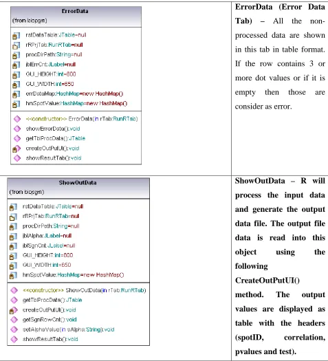
ErrorData (Error Data
Tab) – All the
non-processed data are shown
in this tab in table format.
If the row contains 3 or
more dot values or if it is
empty then those are
consider as error.
ShowOutData – R will
process the input data
and generate the output
data file. The output file
data is read into this
object using the
following
CreateOutPutUI()
method. The output
values are displayed as
table with the headers
(spotID, correlation,
[image:44.612.85.562.70.595.2]PlotGraph – Processed R
data are shown as graph.
createChart() method is
initiated which plots the
GraphDataset – It is part
of JFreeChart jar file. This
object is extended in
PlotGraph object to plot a