Conceptual Framework for Invariant Protein
Fragment Library
Sapna V. M, Roshan Makam, Keshava M, Sudhanva Narayna
Abstract: Proteins are essential and are present in all life forms and determining its structure is cumbersome, laborious and time consuming. Hence, over 3-4 decades, researchers have been using computational techniques such as template and template free based protein structure prediction from its sequence. This research focuses on developing a conceptual basis for establishing an invariant fragment library which can be used for protein structure prediction. Based on 20 amino acids, fragments can be classified into lengths of 3 to 41 size. Further, they can be classified based on the identical number of amino acids present in the fragment. This encompasses theoretically the number of fragments that can exist and in no way represent the actual possible fragments that can exist in nature. Invariant fragments are ones which are rigid in structure 3-dimensionally and do not change. A formula was arrived at to determine all possible permutations that can exist for length 3 to 41 based on the 20 amino acids. 100 proteins from the Protein Data Bank were downloaded, broken into fragments of 3 to 41 resulting in a total of 6102,102 fragments using Asynchronous Distributed Processing. Then identical fragments in sequence were superimposed and Root Mean Square Deviation (RMSD) values were obtained resulting in roughly 3.2% of the original framgnets.. t-score and z-scores were obtained from which Skewness, Kurtosis and Excess Kurtosis were determined. For invariance, skewness cutoff was set at + 0.1 and using the excess kurtosis, fragments whose distribution were either leptokurtic or platykurtic and were within + 1 standard deviation of the mean value were considered as invariant i.e., if there were no outliers in the distribution and if most of the t-score or z-score values were centered around its average value. Using these cutoff values, fragments were classified and deposited into an invariant fragment library. Roughly 3,81,799 invariant fragments were obtained which is roughly 6.3% of the total number of initial fragments. This would be way less than the number of fragments that one has to either use in homology or de-novo modelling thereby reducing the design space. Further work is underway to set up the entire invariant fragment library which can then be used to predict protein structure by template-based approach.
Keywords: Proteins, Fragments, Invariant, Library
I. INTRODUCTION
Proteins are ubiquitous in all life forms and are structurally classified into primary, secondary, tertiary and quaternary structures [1]. In order to form a conformational structure, a protein has an astronomical number of possible conformations due to a very large number of degrees of
Revised Manuscript Received on December 12, 2019. Corresponding Author
Sapna V. M, Assistant Professor & Research Scholar, Biotechnology Department, PES University, 100 Feet Ring Road, BSK 3rd Stage, Bangalore – 560085
Roshan Makam, Biotechnology Department, PES University, 100 Feet Ring Road, BSK 3rd Stage, Bangalore – 560085
Keshava M,Biotechnology Department, PES University, 100 Feet Ring Road, BSK 3rd Stage, Bangalore – 560085
Sudhanva Narayna, Biotechnology Department, PES University, 100 Feet Ring Road, BSK 3rd Stage, Bangalore – 560085
Email: sapnavmk@gmail.com, Mob: 919503212139
freedom in an unfolded polypeptide chain as noted in 1969 by Cyrus Levinthal which is now well known as Levinthal paradox [2],[3]. Subsequently in 1972 the thermodynamic hypothesis was stated by Christen Anfinsen which states that the native structure of a protein is determined solely by the sequence of amino acids in its polypeptide chain and represents the state of lowest conformational energy in its native conditions [4],[5]. Protein structure prediction has applications in the field of medicine such as drug design, protein-protein interactions, in the field of industrial enzymes such as detergents, environmental applications such as waste treatment, food industries, agriculture, etc [6],. Ever since a number of methods have been established to predict the conformation of the protein from its primary sequence [7]. These can be broadly classified into template based and template free methods [8]. Homology and threading falls under template-based method and ab-initio or
de-novo falls under template-free method. Each method has its own pros and cons and there has never been a single method which is able to predict all the protein structures [9]. Although the de-novo method is template-free it uses a decoy set of fragments as templates. All these methods use some sort of global energy minimization to predict the protein structure [10]. Template based methods are based on a fragment library of about 7 to 9 fragment length [11],[12]. Hence, this work focuses on providing a theoretical basis of the design space for creating an invariant fragment library.
II. CONCEPTUAL BASIS FOR INVARIANT
FRAGMENT LIBRARY
templates with fixed arrangements? This will then form the basis for invariant fragment library in order to predict protein structure using the template-based approach [17]. Since the protein can be made from a set of 20 amino acids, the templates must be made from an arrangement of these amino acids [18]. The minimum length of the sequence of amino acids to form a structure is 3 in number i.e., if one considers the rigidity of the chain to be like a dumbbell i.e., the middle amino acid is flanked by one other amino acid either of the same kind or different on either side to hold it rigidly in the crystallized form. If one were to continue like this then the maximum length that can be flanked on either side of the central amino acid is 20 as there are only 20 amino acids, giving the chain length of the fragment to be 41. It is worth to note here that the chain length of the protein can be of any number but that of the fragments can be of maximum length of 41.
Next we consider the design space of the fragment library taking into account the 20 amino acids [19]. From above we know that the minimum and maximum chain length of the fragment must be 3 and 41 respectively. Hence the design space must be 203 to 2041 possible arrangements i.e., the 20 amino acids raised to the power of the fragment chain length. Further, the arrangements of each chain length can be further classified into specific combinations meaning that each fragment chain length combination can be arranged by all permutations of the combination.
Consider ‘S ‘as a set of all the 20 amino acids i.e., S = (G,P,A,V,L,I,M,C,R,Y,W,H,K,R,Q,N,E,D,S,T) and the fragment chain length as ‘n’.
For simplicity consider the 3 alphabets as set S1 = (A, B, C). If one were to compute all the possible arrangements of set S1, with a fragment of length 3, then it is 3
3
= 27 possible arrangements. These 27 possible arrangements can be further classified as shown in Table 1.
Number of arrangements of repetitive amino acids Raa, is given by equation 1.
(1)
Where
r - fragment length
k – total number of times unique amino acid is repeating
j – number of unique amino acids repeating
[image:2.595.300.557.49.206.2]Example:
Table 1: Classification of arrangements of fragment length 3
Type Classification Arrangement Total
All of 3 AAA, BBB, CCC 3
the same kind Two of the same kind and one of different kind
2, 1 AAB, ABA, BAA
BBA, BAB, ABB AAC, ACA, CAA CCA, CAC’, ACC BBC, BCB, CBB CCB, CBC, CBB
18
All of different kind
1, 1, 1 ABC, ACB, BAC
BCA, CAB, CBA
6
Total 27
Number of combinations Caa, of n amino acids is given by equation 2.
(2)
Where
n - total number of amino acids in set S1 j – number of unique amino acids repeating
Example:
Number of permutations for switching Saa, is given by equation 3.
(3)
Where
j – number of unique amino acids repeating Lx – count of identical numbers of k1, k2, ……, kj repeating in equation 1
Example:
Therefore, for a particular classification, the total number of permutations that can occur for a fragment of length r in set S is given by N from equation 4:
(4)
Where
M - total number of permutations for a particular
classification
Raa – number of permutations for repetitive amino
acids by equation 1
by equation 2
Saa – number of permutations for switching by
equation 3
Example:
Hence, the total number of permutations that are occurring for a fragment of length 3 in subset S1 for classification of 2,1 is 3x3x2 = 18
Considering all the 20 amino acids and for a fragment length of 3, the total number of permutations/arrangements is given in Table 2.
Table 2: Total arrangements of 20 amino acids for a fragment length of 3 for different classifications Fragment Classification Theoretical Permutations
3 20
2, 1 1140
1, 1, 1 6840
Total 8000
A similar classification based on the 20 amino acids can be extended to fragment lengths 3 to 41 which covers the entire design space (203 to 2041) theoretically. This does not mean that all fragments exist in nature or in the Protein Data Bank. Also, the possibility exists that a fragment can exist multiple times. This leads us to find variant and invariant fragments.
III. DETERMINATION OF VARIANT AND
INVARIANT FRAGMENTS
Variant and Invariant Fragments are determined based on statistical measures viz., Skewness, Kurtosis and Excess Kurtosis. If we consider a fragment to have multiple copies of the same fragment, then superimposing the fragments on one another will give us values of Root Mean Square Deviation (RMSD) [20],[21]. A value of RMSD equal to zero indicates that the superimposition is a perfect one and value of RMSD greater than zero indicates the deviation exists between the fragment being superimposed with the reference fragment. If one were to plot the number of times for a particular fragment with respect to RMSD, one obtains a histogram or frequency distribution curve. Further, for each fragment a t-distribution for a set of samples or z-distribution in the case of population is obtained using equation 5 and 6 respectively.
(5)
Where RMSD - Root Mean Square Deviation of a single sample in the sample set for a particular
fragment
RMSDmean - Mean of the Root Mean Square Deviation of the sample set for a particular
fragment
s - standard deviation of the sample set for a
particular fragment
n – total number of samples in the sample set for a
particular fragment
(6)
Where = standard deviation of the population for a
particular fragment
The tfragment normalizes the RMSD values between -3 to +3 with an average or mean equal to zero. Hence, if one were to compute the tfragment values for all the sample sets of the fragment then one can determine the invariance or variance of a fragment using Skewness and Excess Kurtosis.
Skewness is a measure of the symmetry or more precisely, the lack of symmetry of the frequency distribution [22]. If it is positively skewed then the curve has a longer tail on the right hand side of the curve and if it is negatively skewed then the curve has a longer tail on the left hand side of the curve and if the skewness is zero then it is a perfectly bell-shaped curve with symmetry about the average or mean value [23]. Skewness is determined by equation 7 as follows:
(7)
where RMSD, RMSDmean, n and s represent the usual meaning.
Kurtosis is a measure of the relative sharpness of the peak of a frequency distribution [23]. It is used to indicate the flatness or peakedness of the frequency distribution. Positive kurtosis represents that the distribution is more peaked than the normal distribution whereas negative kurtosis shows that the distribution is less peaked than the normal distribution. Excess kurtosis is a metric that measures the kurtosis of a distribution against the kurtosis of a normal distribution and is given by Excess Kurtosis = Kurtosis – 3. If the excess kurtosis is zero or close to zero, then the distribution follows a normal distribution and is called as mesokurtic distribution. If the excess kurtosis is positive, then the distribution shows heavily tailed on either side and is called leptokurtic distribution [24]. If the excess kurtosis is negative, then the tails of the distribution is flat and is called platykurtic distribution. Excess Kurtosis for a population is determined by equation 8 as follows:
- 3 (8)
where RMSD, RMSDmean, n and s represent the usual meaning.
And Sample Excess Kurtosis is given by equation 9 as follows:
Ideally an invariant fragment must be without a distribution otherwise the fragment is variant. This means that the invariant fragment must have identical or near identical RMSD value with the average RMSD being equal to the RMSD value itself indicating that the distribution must not have any outliers. This is rarely possible in reality and hence the statistical measures are used such as skewness and excess kurtosis. The RMSD values must ideally be centered around its average value. The invariant fragment represents rigidness of the fragment conformationally in the 3-dimensional space and represents a fixed state and hence can be used to predict protein structures.
IV. METHODOLOGY
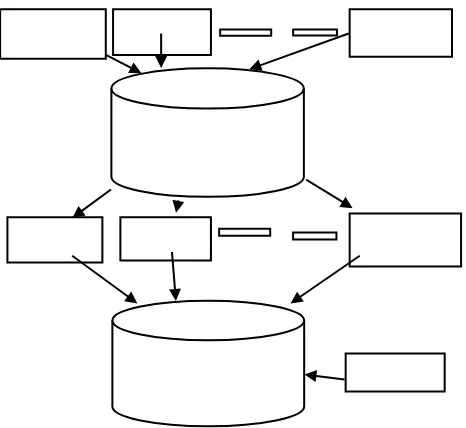
Computer Configuration consisted of two nodes with each node consisting of 16 cores, 128 GB RAM and a storage space of 133 GB. Node 1 and Node 2 were treated as master and slave respectively. Following software were installed on Node 1: Redis, SQL, Python, Numpy and Celery Package. Node 2: Python, Numpy and Celery Package and is listed in Table 3. Figure 1 shows the basic architecture of the entire process. Figure 2 shows the overall flowchart from taking protein sequences, breaking it into fragments of 3 to 41, superimposing the structures of identical sequences, determining the invariance and depositing into the database.
The following python scripts (not shown) tab.py (defines tables and classes), config.py (configures SQL Alchemy) and db.py (to create and destroy tables) were written. SQL ALCHEMY facilitates the communication between the python scripts the databases. ORM is the one that translates python classes to tables on databases and automatically converts function calls to SQL statements
Table 3: Software Packages installed on Nodes 1 and 2
Sl.No Software Installation (Packages)
Version
1 Operating system- Ubuntu 16.04
2 Anaconda Custom
3 Python 3.6.4
4 Biopython 1.70 or 1.71
5 Numpy 1.13.1 or 1.14.2
6 Redis 5.0.3
Redis Server 2.4.5
7 MySQL Shell 8.0.11
SQL Alchemy 1.3.0 or 1.2.1
8 Celery 4.2 or 4.0
[image:4.595.40.524.84.768.2]Fig 1. Basic Architecture between Python scripts and the Database
Fig 2. Overall Flow Chart for Invariant Database No
No Yes
Database Invariant Database
Statistical analysis(Skewness
and Kurtosis) Superimpose structures to get
RMSD Values Compare fragments of equal length and
100% identity Break structure into size 3 to 41 fragments and put in tab 3 to 41
Get structure Input PDB ID:Sequence file(CSV file)
For every PDB
Fig 3. Internal PDB Processing - Asynchronous Distributed Processing
Figure 3 shows the Asynchronous Distributed Processing between the producers and workers for processing the protein (PDB) files to the invariant database
CELERY PACKAGE: An open source asynchronous task queue/job queue based on distributed message passing. The execution units called tasks are executed concurrently on one or more workers nodes. Celery requires a solution to send and receive messages; usually this comes in the form of a separate service
called a message broker [26]. The message broker here
is REDIS and database is SQLALCHEMY [27]
Producers: Pushes tasks and queues them on to Redis and initiates the workers to perform the tasks(processor.py)
Calling tasks is done using delay( ) method
Redis: Holds the path of PDB to break into fragments and holds the residues and its details in the Key-Value form [28].
Workers: Performs Breaking into fragments of size 3 to 41, putting into database, identifying identical fragments, superimpose the similar fragments to generate RMSD values for all possible combinations and extract fragment combinations with min RMSD value.
V. RESULTS AND DISCUSSIONS
A sample of 100 PDBs were downloaded from the Protein Data Bank [25]. The proteins were fragmented from 3 to 41 lengths. A total of 61,02,012 fragments were obtained. The fragments which were identical in sequence were then superimposed in the 3-dimensional space using the Cartesian coordinates from the respective PDBs, the RMSD values were obtained and the tfragment values were determined. A frequency distribution curve was developed using the tfragment values for that particular fragment and Skewness, Kurtosis and Excess Kurtosis were calculated.
After superimposition the total number of unique fragments obtained was 1,94,197. We have to bear in mind that this is not the entire data set of proteins from the Protein Data Bank but a sample of 100 proteins.
Table 4 shows the data for all the fragments created before and after superimposition. One can see that prior to superimposition the number of fragments is high compared to the number of fragments after superimposition.
Table 5 is a snapshot of data analysis for fragment size 3. Each fragment was grouped for repetition and is listed as fragment, fragment type, the number of repetitions of that particular fragment, the average or mean t-score value and its standard deviation from which the skewness and excess kurtosis has been calculated. For most of the data the skewness was less than + 1 indicating that the data was
Table 4: Number of Fragments before and after superimposition
Fragment Size
Number of Fragments
Number of unique
Fragments Fragment Size
Number of Fragments
Number of unique Fragments
3 376482 4993 23 148718 4793
4 234386 7221 24 145183 4736
5 218881 6443 25 141648 4678
6 108153 6225 26 138172 4621
7 209329 6104 27 134699 4567
8 205232 5990 28 131415 4514
9 201174 5879 29 128139 4465
10 197135 5779 30 124969 4417
11 193144 5683 31 121799 4369
12 189165 5591 32 118981 4324
13 185230 5507 33 116264 4282
14 181304 5430 34 113548 4241
15 177387 5351 35 110832 4200
16 173758 5271 36 108153 4161
17 170134 5196 37 105477 4125
18 166549 5122 38 102808 4089
19 162968 5049 39 100272 4053
20 159391 4978 40 97775 4014
21 155817 4910 41 95286 3976
22 152255 4850
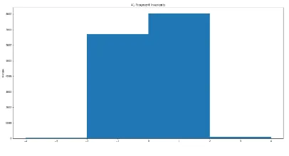
[image:5.595.299.554.279.637.2]In order to determine the invariance of the fragments, the cutoff for skewness was kept to +0.1. For invariance, however in case of kurtosis the fragments must not have any outliers and at the same time must have a sharp and very high peak at the average value indicating that all the repetitive fragments lie very close to the mean value. The cutoff for skewness and kurtosis were based on the mean or average values of the t-score values for each fragment size and its standard deviation must be less than 10% of the mean value chosen randomly. Keeping this as the basis, all the fragments with lengths from 3 to 41 were classified into variant and invariant and were deposited into a database library (data not shown). Figures 4a, 5a, and 6a shows examples of the variant fragments for length 3, 21, 41 respectively and Figures 4b, 5b and 6b shows examples of the invariant sample fragments for length 3, 21 and 41 respectively.
Table 5: Snapshot of Data Analysis for Fragment Size 3
Fragmen t
Fragmen t type N
Mea n
Standar d deviatio
n
Ske w
Kurtosi s
AAA 3
32
5 0.864 0.729 0.40
3 -1.6
AAR 21 91 1.488 0.498
-0.58
1 0.135
AAN 21 21 0.662 0.287
-0.32
6 -1.022
AAD 21
12
0 1.274 0.859 0.11
2 -1.473
AAQ 21 6 0.845 0.363
-0.87
6 -0.479
AAE 21 36 1.314 0.509
0.17
5 -1.006
AAG 21
10
5 1.201 0.387 -0.94
9 0.647
AAH 21 3 1.345 0.522
-0.70
1 -1.5
AAI 21 10 0.474 0.239 0.4 -1.765
AAL 21
17
1 0.844 0.402 -0.25 -1.104
AAK 21 46 1.357 0.586
0.16
2 -0.863
AAM 21 10 0.875 0.328
-0.54
6 -0.301
AAF 21
75
8 0.22 0.551 3.36
8 10.573
AAP 21 1 2.287 0 0 0
AAS 21 78 1.137 0.631
0.23
8 -0.791
[image:6.595.327.527.210.312.2]Based on the above definition of invariant and variant fragment, from 61,02,012 fragments, a total of 3,81,799 invariant fragment which is roughly 6.3% of the initial fragments were obtained. This Is way less in the design space than the number of fragments that are used for homology or de novo modelling of protein structure prediction.
Fig. 4a: Variant Fragment for length of size 3
[image:6.595.44.291.265.646.2]Fig. 4b: Invariant Fragment for length of size 3
[image:6.595.43.295.270.648.2]Fig. 5a: Variant Fragment for length of size 21
[image:6.595.325.526.361.474.2] [image:6.595.328.527.510.612.2]Fig. 6a: Variant Fragment for length of size 41
Fig. 6b: Invariant Fragment for length of size 41
VI. CONCLUSION
A conceptual basis based on the length of the fragment and statistical analysis of the RMSD values for all the superimposed fragments of proteins from length 3 to 41 such as Skewness and Excess Kurtosis were established for 100 proteins. The proteins were broken into fragments of 3 to 41, superimposed for identical fragment sequences and an invariant fragment library was established. From a total of 61,02,012 fragments, the fragments were reduced to 3.2% from which it was further reduced to 3,81,799 invariant fragments which roughly 6.3% of the initial number of fragments from 100 proteins. In conclusion, we can say that such an undertaking has not be considered before when using homology or de-novo methods of protein structure prediction where the design space is humungous and hence an attempt is made to reduce the design space for protein structure prediction.
FURTHER SCOPE AND FUTURE WORK Based on the above work of setting up an invariant fragment library, work is underway to establish the entire database from all the proteins in the Protein Data Bank. Further, protein structure prediction using this invariant fragment library is being set up.
ACKNOWLEDGMENT
The authors would like to acknowledge the management and staff of PES University. The authors are thankful to Mr. Subash Reddy, the librarian of PES University for supportive service to prepare the manuscript
REFERENCES
1. Lesk, A. M. (2001). Introduction to protein architecture: the
structural biology of proteins. Oxford: Oxford University Press.
2. Levinthal, C. (1968). Are there pathways for protein folding? Journal de chimie physique, 65, 44-45.
3. Zwanzig, R., Szabo, A., & Bagchi, B. (1992). Levinthal's paradox. Proceedings of the National Academy of Sciences, 89(1), 20-22. 4. Anfinsen, C. B. (1973). Principles that govern the folding of protein
chains. Science, 181(4096), 223-230.
5. Dill, K. A., & Chan, H. S. (1997). From Levinthal to pathways to funnels. Nature Structural and Molecular Biology, 4(1), 10 6. Vallat, B., Madrid-Aliste, C., & Fiser, A. (2015). Modularity of
protein folds as a tool for template-free modeling of structures. PLoS computational biology, 11(8), e1004419
7. Ramyachitra, D., & Veeralakshmi, V. (2014). Computational Analysis of Protein Structure Prediction and Folding. Int. J. Comput. Sci. Inform. Technol. Secure, 4, 116-127
8. Deng, H., Jia, Y., & Zhang, Y. (2018). Protein structure prediction. International Journal of Modern Physics B, 32(18), 1840009
9. Sapna V M, Roshan Makam, V K Agrawal (2018)
Protein Structure Determination and Prediction: A Review of Techniques International Journal of Recent Research and Review, Vol. XI, Issue 3, September 2018 ISSN 2277 – 8322
10. Liwo, A., Lee, J., Ripoll, D. R., Pillardy, J., & Scheraga, H. A. (1999). Protein structure prediction by global optimization of a potential energy function. Proceedings of the National Academy of Sciences, 96(10), 5482-5485
11. Du, P., Andrec, M., & Levy, R. M. (2003). Have we seen all structures corresponding to short protein fragments in the Protein Data Bank? An update. Protein Engineering, 16(6), 407-414. 12. Sander, O. (2004). Local sequence-structure relationships in proteins
(Doctoral dissertation, Friedrich-Alexander-Universität Erlangen-Nürnberg Erlangen-Erlangen-Nürnberg).
13. Pauling, Linus, Robert B. Corey, and Herman R. Branson. "The structure of proteins: two hydrogen-bonded helical configurations of
the polypeptide chain."Proceedings of the National Academy of
Sciences37.4 (1951): 205-211.
14. Bowie, J. U., Luthy, R., & Eisenberg, D. (1991). A method to identify protein sequences that fold into a known three-dimensional structure. Science, 253(5016), 164-170.
15. Lesk, A. M. (2001). Introduction to protein architecture: the structural biology of proteins. Oxford: Oxford University Press. 16. Alberts, B., Johnson, A., Lewis, J., Raff, M., Roberts, K., & Walter,
P. (2002). The shape and structure of proteins
17. Szilagyi, A., & Zhang, Y. (2014). Template-based structure modeling of protein–protein interactions. Current opinion in structural biology, 24, 10-23
18. Lee, J., Lee, J., Sasaki, T. N., Sasai, M., Seok, C., & Lee, J. (2011). De novo protein structure prediction by dynamic fragment assembly and conformational space annealing. Proteins: Structure, Function, and Bioinformatics, 79(8), 2403-2417.
19. Xu, D., & Zhang, Y. (2012). Ab initio protein structure assembly using continuous structure fragments and optimized knowledge‐based force field. Proteins: Structure, Function, and Bioinformatics, 80(7), 1715-1735
20. Kumar, N. J. (2013). DIVISION OF MATRICES AND MIRROR IMAGE PROPERTIES OF MATRICES. International Journal of Advancements in Computing Technology, 2(7), 431.
21. Skolnick, J., & Kihara, D. (2001). Defrosting the frozen approximation: PROSPECTOR—a new approach to threading. Proteins: Structure, Function, and Bioinformatics, 42(3), 319-331. 22. Norman, G. R., & Streiner, D. L. (2008). Biostatistics: the bare
essentials. PMPH USA
23. Vittinghoff, E., Glidden, D. V., Shiboski, S. C., & McCulloch, C. E. (2011). Regression methods in biostatistics: linear, logistic, survival, and repeated measures models. Springer Science & Business Media. 24. Ryu, E. (2011). Effects of skewness and kurtosis on normal-theory
based maximum likelihood test statistic in multilevel structural equation modeling. Behavior research methods, 43(4), 1066-1074. 25. https://www.rcsb.org/stats/growth/overall
26. https://docs.celeryproject.org/en/latest/getting-started/introduction.html
27. https://auth0.com/blog/sqlalchemy-orm-tutorial-for-python-developers/
[image:7.595.68.271.210.320.2]AUTHORSPROFILE
First Author: Sapna V M currently working as Assistant Professor at Dayananda Sagar University, Bangalore. She is pursuing her PhD at PES University, Bengaluru and working on protein structure prediction. She has served as Research Scholar at PES University, Research Associate at KAnOE, PES University, Bengaluru for two years, Assistant professor at MITCOE Department of IT, Pune for five years, and Lecturer at DSI Department of IT for a year, Bengaluru. She has four publications to her credit. Her interests include bioinformatics and computational biology, Database management systems, Software engineering, Artificial intelligence and Machine learning.
Second Author: Dr Roshan Makam is the Professor and Ex-Chairperson of Biotechnology Department at PES University, Bengaluru. He has over 25+ years of experience in industry and academia. He has both MS and PhD from Arizona State University and has several patents and publications to his credit. His interests include bioinformatics and computational biology. He is a reviewer of 7 international journals and an Editor of Reviews in Bioinformatics
Third Author: Keshava M was a research scholar in the Biotechnology Department at PES University, Bangalore. He has completed his MSc. Engg. By Research at VTU, Belgaum. He has interests lie in Bioinformatics, Protein Structure Prediction and Computational Biology.