Visualization of Large High Dimensional Data via Interpolation Approach of Multidimensional Scaling

Visualization of Large High-Dimensional Data

via Interpolation Approach of Multidimensional Scaling

Seung-Hee Baea,∗, Judy Qiua,b_{, Geoffrey Fox}a,b

a_{Pervasive Technology Institute at Indiana University, 2719 E. 10th St., Bloomington, IN, 47408, United States} b_{School of Informatics and Computing at Indiana University, 901 E. 10th St., Bloomington, IN, 47408, United States}

Abstract

The recent explosion of publicly available biology gene sequences and chemical compounds offers an unprecedented opportunity for data mining. To make data analysis feasible for such a vast volume and high-dimensional scientific data, we can apply high performance dimension reduction algorithms. Among the known dimension reduction algorithms, we utilize the multidimensional scaling (MDS) algorithm to configure given high-dimensional data into the target dimension. However, the MDS algorithm re-quires a quadratic order of memory as well as computing resources, and it is usually infeasible to deal with millions of points via normal MDS method even under a commodity cluster system with distributed-memory. Thus, the authors propose a method of interpolation to utilize the mapping of only a small subset of the given data. This approach effectively reduces computational complexity. With minor trade-offin approximation, our interpolation method makes it possible to process millions of data points with only modest amounts of computation and memory. Since huge amount of data are involved, we show how to parallelize the proposed MDS interpolation algorithm as well. For the evaluation of the interpolated MDS by STRESS criteria, it is necessary to compute STRESS value. The STRESS value calculation involves symmetric matrices generated by all pairwise computation, but each process only accesses a subset of the data required. Thus, we also propose a simple but efficient parallel mechanism for symmetric pairwise computation when only a subset of data is available to each process. Our experimental results illustrate that the quality of interpolated mapping results are comparable to the mapping results of full MDS algorithm only. With respect to parallel performance, those interpolation methods are well parallelized and have high efficiency. With the proposed MDS interpolation method, we construct a configuration of four-million out-of-sample data in the target dimension, and the number of out-of-sample data can be increased further.

Keywords: Multidimensional Scaling, Interpolation, Dimension Reduction, Data Visualization

1. Introduction

Due to the advancements in science and technology over the last several decades, every scientific and technical field has gen-erated a huge amount of data such that we find ourselves in the era of data deluge. Data-intensive scientific computing [1] has emerged and has been attracting increasing numbers of people. To analyze the incredible amount of data, many data mining and machine learning algorithms have been developed. Among the many data mining and machine learning algorithms, we focus on dimension reduction algorithms, which reduce data dimen-sionality from original high dimension to target dimension, in this paper.

Among the many dimension reducing algorithms that exist, such as principle component analysis (PCA), generative topo-graphic mapping (GTM) [2, 3], self-organizing map (SOM) [4], and multidimensional scaling (MDS) [5, 6], we have worked on MDS in this paper. We previously parallelize the MDS al-gorithm to utilize multicore clusters and to increase the com-putational capability with minimal overhead for the purpose of

∗_{Corresponding author}

Email addresses:[email protected](Seung-Hee Bae),

[email protected](Judy Qiu),[email protected](Geoffrey Fox)

investigating large data sets, such as 100,000 data [7]. How-ever, parallelization of an MDS algorithm, whose computa-tional complexity and memory requirement goes up toO(N2) where N is the number of points, is still limited by the mem-ory requirement for huge amounts of data, e.g. millions of points, although it utilizes distributed memory environments, such as clusters, for acquiring more memory and computational resources. In this paper we try to solve the memory-bound problem by applying an interpolation method based on pre-configured mappings of the sample data for the MDS algorithm, so that we can provide configurations for millions of points in the target space.

This paper is an extension of the MDS interpolation sections in our conference paper [8], and this paper illustrates much more detailed experimental investigations and analyses of the proposed MDS interpolation. 1 _{This paper is organized as}

fol-lows: We begin with a brief discussion of the existing methods for addressing the out-of-sample problem in various dimension reduction algorithms and the concept of the multidimensional

scaling (MDS) in Section 2 and Section 3, repectively. Then, the proposed interpolation method and how to parallelize it are described in Section 4. Various experimental analyses, which are related to the proposed MDS interpolation algorithm, are shown in Section 5, followed by our conclusion and future work in Section 6.

2. Related Work

The out-of-sample method, which embeds new points with respect to previously configured points, has been actively re-searched for recent years, and it aims at improving the capabil-ity of dimension reduction algorithms by reducing the require-ments of computation and memory with the trade-offof slightly approximated mapping results.

In a sensor network localization field, when there are only a subset of pairwise distances between sensors and a subset of anchor locations available, people try to find out the loca-tions of the remaining sensors. For instance, the semi-definite programming relaxation approach and its extended approaches have been proposed to solve this issue [9]. Bengio et. al. [10] and Trosset et. al. [11] proposed out-of-sample extension for the classical multidimensional scaling (CMDS) [12], which is based on spectral decomposition of a symmetric positive semi-definite matrix (or the approximation of positive semi-semi-definite matrix), and the embeddings in the configured space are repre-sented in terms of eigenvalues and eigenvectors of it. Bengio et. al. [10] proposed a method which projects the new point x onto the principal components, and Trosset et. al. [11] extended the CMDS algorithm itself to the out-of-sample problem. Trosset et. al. described, in their paper [11], how to embed one point between the embeddings of the original n objects through mod-ification of the original CMDS equations, which preserves the mappings of the original n objects, by using (n+1)×(n+1) ma-trix A2instead of n×n matrix∆2, and the authors showed how

to configure a number of points simultaneously by using matrix operations. Recently, a multilevel force-based MDS algorithm was proposed as well [13].

In contrast to applying the out-of-sample problem to CMDS, I extend the out-of-sample problem to general MDS results with the STRESS criteria of Eq. (1), which finds embeddings with respect to the distance (or dissimilarity) rather than to the in-ner product as in CMDS, with an gradient descent optimization method, called iterative majorizing. The proposed iterative ma-jorizing interpolation approach for the MDS problem will be explained in Section 4.

3. Multidimensional Scaling (MDS)

“Multidimensional scaling” (MDS) [12, 5, 6] is a term that refers to techniques for constructing a map of generally high-dimensional data into a target dimension (typically a low di-mension) with respect to the given pairwise proximity infor-mation, while each distance between a pair of points in the generated mapping is approximated to the corresponding dis-similarity value as much as possible. Mostly, MDS is used to

visualize given high dimensional data or abstract data by gen-erating a configuration of the given data that utilizes Euclidean low-dimensional space, i.e. two or three dimension.

Generally, proximity information, which is represented as an

N×N dissimilarity matrix (∆=[δi j]), where N is the number of

points (objects) andδi jis the dissimilarity between point i and j,

is given for the MDS problem, and the dissimilarity matrix (∆) should agree with the following constraints: (1) symmetricity (δi j =δji), (2) non-negativity (δi j ≥0), and (3) zero diagonal

elements (δii = 0). The output of the MDS algorithms could

be represented as an N×L configuration matrix X whose rows

represent each data point xi (i = 1, . . . ,N) in L-dimensional

space. It is quite straightforward to compute the Euclidean distance between xi and xj in the configuration matrix X, i.e. di j(X) = kxi−xjk, and we are able to evaluate how well the given points are configured in the L-dimensional space by us-ing the suggested objective functions of MDS: STRESS [14] or SSTRESS [15]. Definitions of STRESS (1) and SSTRESS (2) are following:

σ(X) = X

i<j≤N

wi j(di j(X)−δi j)2 (1)

σ2(X) = X

i<j≤N

wi j[(di j(X))2−(δi j)2]2 (2)

where 1≤i< j≤N and wi jis a weight value, so wi j≥0.

As shown in the STRESS and SSTRESS functions, the MDS problem could be considered as a non-linear optimiza-tion problem, which minimizes either the STRESS (σ(X)) or the SSTRESS (σ2_{(X)) function in the process of configuring an} L-dimensional mapping of the high-dimensional data.

4. Majorizing Interpolation MDS

One of the main limitations of most MDS applications is that they requireO(N2_{) memory as well as O(N}2₎

computa-tion. Thus, though it is possible to run them with a small data set without any trouble, it is impossible to execute them with a large number of points due to memory limitations; therefore, this challenge could be considered to be a memory-bound problem as well as a computing-memory-bound problem. For instance, Scaling by MAjorizing of COmplicated Function (SMACOF) [16, 17], a well-known MDS application based on iterative majorization method which is similar to Expectation-Maximization (EM) [18] approach, uses six N×N matrices. If N=100,000, then one N×N matrix of 8-byte double-precision

numbers requires 80 GB of main memory, so the algorithm needs to acquire at least 480 GB of memory to store these six

N×N matrices. It is possible to run a parallel version of

To solve this obstacle, we develop a simple interpolation ap-proach based on the pre-mapped MDS result of the sample of the given data. Our interpolation algorithm is similar to the

k nearest neighbor (k-NN) classification [19], but we

approx-imate a new mapping position of the new point based on the positions of k-NN, among pre-mapped subset data, instead of classifying it. For the purpose of deciding a new mapping posi-tion in relaposi-tion to the k-NN posiposi-tions, the iterative majorizaposi-tion method is applied as in the SMACOF [16, 17] algorithm. The details of mathematical majorization equations for the proposed out-of-sample MDS algorithm are shown below. The algorithm proposed in this paper is called Majorizing Interpolation MDS (hereafter MI-MDS).

The proposed algorithm is implemented as follows. We are given N data points in a high-dimensional space, say D-dimension, and proximity information (∆=[δi j]) on those data

as in Section 3. Among the N data points, the configuration of the n sample points in L-dimensional space, x1, . . . ,xn ∈ RL,

called X, are already constructed by an MDS algorithm; here we use the SMACOF algorithm. Then, we select k nearest neighbors ( p₁, . . . ,p_k ∈ P) of the given new point among the

n pre-mapped points with respect to correspondingδix, where

x represents the new point. We use a linear search to find the

k-nearest neighbors among n-sampled data, so that the

com-plexity of finding the k-nearest neighbors isO(n) per one inter-polated point (here x). Finally, the new mapping of the given new point x ∈ _RL _{is calculated based on the pre-mapped}

po-sition of the selected k-NN and the corresponding proximity informationδix. Finding new mapping position is an

optimiza-tion problem which minimize STRESS (3) value with m points, where m=k+1. However, only one point x is movable among

m points, so we can simplify the STRESS equation (3) as

fol-lows (Eq. (4)), and we set wi j =1, for∀i,j in order to simplify.

σ(X) = X

i<j≤m

(di j(X)−δi j)2 (3)

= C+

k

X

i=1 d2_ix−2

k

X

i=1

δixdix (4)

whereδixis the original dissimilarity value between piand x, dixis the Euclidean distance in L-dimension between p_iand x, andCrepresents a constant part. The second term of Eq. (4) can be deployed as following:

k

X

i=1

d2_ix = kx−p1k 2

+· · ·+kx−pkk 2

(5)

= kkxk2+

k

X

i=1

kp_ik2−2xtq (6)

where qt _{= (}Pk

i=1pi1, . . . ,

Pk

i=1piL) and pi jrepresents the j-th

element of p_i. In order to establish majorizing inequality, we apply the Cauchy-Schwarz inequality to−dixof the third term of Eq. (4). Please, refer to chapter 8 in [6] for details of how to apply the Cauchy-Schwarz inequality to−dix. Since dix =

kp_i−xk,−dixcould have the following inequality based on the

Cauchy-Schwarz inequality:

−dix ≤

PL

a=1(pia−xa)(pia−za)

diz (7)

= ( pi−x)

t_{( p} i−z) diz

(8)

where zt=(zi, . . . ,zL) and diz=kpi−zk. The equality in Eq. (7)

occurs if x and z are equal. If we apply Eq. (8) to the third term of Eq. (4), then we obtain

−

k

X

i=1

δixdix ≤ −

k

X

i=1

δix diz

( p_i−x)t( p_i−z) (9)

= −xt

k

X

i=1

δix

diz(z−pi)+Cρ (10)

whereCρ is a constant. If Eq. (6) and Eq. (10) are applied to

Eq. (4), then it could be expressed as:

σ(X)=C+

k

X

i=1 d2_ix−2

k

X

i=1

δixdix (11)

≤ C+kkxk2−2xtq+

k

X

i=1

kp_ik2

−2xt

k

X

i=1

δix

diz(z−pi)+Cρ (12)

=τ(x,z) (13)

where both C and Cρ are constants. In Eq. (13), τ(x,z),

a quadratic function of x, is a majorization function of the STRESS. By setting the derivative ofτ(x,z) equal to zero, we can obtain a minimum; that is

∇τ(x,z)=2kx−2q−2

k

X

i=1

δix

diz(z−pi)=0 (14)

x=

q+Pk_i=1δix

diz(z−pi)

k (15)

where qt =(Pk_i=1pi1, . . . ,Pk_i=1piL), pi jrepresents the j-th

ele-ment of pi, and k is the number of the nearest neighbors that we

selected.

The advantage of the iterative majorization algorithm is that it produces a series of mappings with non-increasing STRESS values as proceeds, which results in local minima. It is good enough to find local minima, since the proposed MI-MDS algo-rithm simplifies the complicated non-linear optimization prob-lem to a small one, such as a non-linear optimization probprob-lem of

k+1 points, where k≪N. Finally, if we substitute z with x[t−1]

x[t]=

q+Pk_i=1δix

diz(x

[t−1]_−p i)

k (16)

x[t]=p+1

k k

X

i=1

δix diz(x

[t−1]₋

pi) (17)

where diz = kpi−x[t−1]kand p is the average of k-NN’s

map-ping results. Eq. (17) is an iterative equation used to embed a newly added point into target-dimensional space, based on pre-mapped positions of k-NN. The iteration stop condition is essentially the same as that of the SMACOF algorithm, which is

∆σ(S[t])=σ(S[t−1])−σ(S[t])< ε, (18)

where S=P∪ {x}andεis the given threshold value.

The time complexity of the proposed MI-MDS algorithm to find the mapping of one interpolated point is O(k) on the basis of Eq. (17), if we assume that the number of iterations required for finding one interpolated mapping is very small. Since finding nearest neighbors takes O(n) and mapping via MI-MDS requires O(k) for one interpolated point, the over-all time complexity to find mappings of overover-all out-of-sample points (N −n points) via the proposed MI-MDS algorithm is

O(kn(N−n)) ≈ O(n(N−n)) due to the fact that k is usually

negligible compared to n or N.

The process of the overall out-of-sample MDS with a large dataset could be summarized by the following steps: (1) Sam-pling; (2) Running MDS with sample data; and (3) Interpolating the remaining data points based on the mapping results of the sample data.

Alg. 1 describes the summary of the proposed MI-MDS al-gorithm for interpolation of new data, say x, in relation to the pre-mapped results of the sample data. Note that the algorithm uses p as an initial mapping of the new point x[0] unless ini-tialization with p makes dix = 0, since the mapping is based

on k-NN. p makes dix=0, if and only if all the mapping

posi-tions of the k-NNs have the same position. If p makes dix =0

(i =1, . . . ,k), then we generate a random variation from the p

point with the average distance ofδ_{ixas an initial position of}

x[0]_.

4.1. Parallel MI-MDS Algorithm

Suppose that among N points the mapping results of n sample points are given in the target dimension, say the L-dimension, so that we could use those pre-mapped results of

n points via MI-MDS algorithm which is described above to

embed the remaining points (M = N−n). Though the

inter-polation approach is much faster than running the MDS algo-rithm, i.e. O(Mn+n2_{) vs. O(N}2_{), implementing parallel}

MI-MDS algorithm is essential, since M can be still huge – in the millions. Additionally, most clusters are now multicore follow-ing the invention of the multicore-chip, so we use hybrid-model parallelism, which combines processes and threads, as seen in various recent papers [20, 1].

Algorithm 1 Majorizing Interpolation MDS (MI-MDS) algo-rithm

1: Find k-NN: find k nearest neighbors of x, pi ∈ P i =

1, . . . ,k of the given new data based on original

dissimi-larityδix.

2: Gather mapping results in target dimension of the k-NN.

3: Calculate p, the average of pre-mapped results of pi∈P. 4: Generate initial mapping of x, called x[0], either p or a

ran-dom variation from p point.

5: Computeσ(S[0]), where S[0]=P∪ {x[0]_}.

6: while t=0 or (∆σ(S[t])> εand t≤MAX ITER) do

7: increase t by one.

8: Compute x[t]_{by Eq. (17).} 9: Computeσ(S[t]).

10: end while

11: return x[t]_;

In contrast to the original MDS algorithm in which the map-ping of a point is influenced by the other points, interpolated points are totally independent of one another – except selected

k-NN in the MI-MDS algorithm, and the independence among

interpolated points makes the MI-MDS algorithm pleasingly-parallel. In other words, MI-MDS requires minimal communi-cation overhead. Also, load-balance can be achieved by using modular calculation to assign interpolated points to each par-allel unit, either between processes or between threads, as the number of assigned points differs by at most one.

4.2. Parallel Pairwise Computation Method with Subset of Data

p1

p5

p4

p3

p2

p5

p4

p3

p2

p1

p1

p2

p3

p4

p5

p1

p2

p3

p4

p5

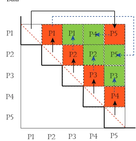
Figure 1: Message passing pattern and parallel symmetric pairwise computa-tion for calculating STRESS values of whole mapping results.

STRESS criteria of Eq. (1) with N points overall, then it re-quiresO(N2_{) computation. Note that we implement our}

hybrid-parallel MI-MDS algorithm as each process has access to only a subset of M interpolated points, without loss of generality M/p

points, as well as the information of all pre-mapped n points. Accessing only a subset of a huge data set spread over clus-ters is a natural way of using a distributed-memory system, e.g. a cluster system, so that each process must communicate with each other for the purpose of accessing all the necessary data to compute STRESS.

In this section we illustrate how to calculate symmetric pair-wise computation efficiently in parallel for the case in which only a subset of data is available for each process. In fact, general MDS algorithms utilize pairwise dissimilarity informa-tion. But suppose we are given N original vectors in the D-dimension, yi, . . . ,yN ∈ Y and yi ∈ RD, instead of a given

dissimilarity matrix like the PubChem fingerprint data that we used for our experiments. In order to calculate the distance in the original D-dimensionδi j =kyi−yjkin Eq. (1), it is

neces-sary to communicate messages between each process to get the required original vectors, say y_iand y_j. Here we used the pro-posed pairwise computation method to measure the STRESS criteria of the MDS problem in Eq. (1), but the proposed par-allel pairwise computation method will be used efficiently for general parallel pairwise computation whose computing com-ponents are independent, such as generating a distance (or dis-similarity) matrix of all data under the condition that each pro-cess can acpro-cess only a subset of the required data.

Fig. 1 describes the proposed scheme when the number of processes (p) is 5, which is an example of the odd number cases. The proposed scheme is an iterative two-step approach, (1) rolling and (2) computing, and the number of iterations is ⌈(1+· · ·+p−1)/p⌉=⌈(p−1)/2⌉. Note that iteration ZERO is calculating the upper triangular part of the corresponding di-agonal block, which does not require message passing. After iteration ZERO is done, each process pi sends the originally

assigned data block to the previous process pi−1 and receives

a data block from the next process pi+1 in a cyclic way. For

instance, process p0 sends its own block to process pp−1 and

receives a block from process p1. This rolling message

pass-ing can be done uspass-ing one spass-ingle MPI primitive per process,

MPI_SENDRECV(), which is efficient. After sending and re-ceiving messages, each process performs computations for the currently assigned pairwise computing block with respect to re-ceiving data and originally assigned block. In Fig. 1 black solid arrows represent each message passings at iteration 1, and or-ange blocks with process IDs are the calculated blocks by the corresponding named process at iteration 1. From iteration 2 to iteration⌈(p−1)/2⌉, the above two-steps are done repeat-edly and the only difference is the sending of a received data block instead of the originally assigned data block. The green blocks and dotted blue arrows show iteration 2, which is the last iteration for the case of p=5.

Also, in case the number of processes is even, the above two-step scheme works in high efficiency. The only difference be-tween the odd number case and the even number case is that two processes are assigned to one block at the last iteration of

Algorithm 2 Parallel Pairwise Computation

1: input: Y=a subset of data;

2: input: p=the number of process;

3: rank⇐the rank of process;

4: sendT o⇐(rank−1) mod p

5: recvFrom⇐(rank+1) mod p

6: k⇐0;

7: Compute upper triangle in the diagonal blocks in Fig. 1;

8: MAX IT ER⇐ ⌈(p−1)/2⌉

9: while k<MAX IT ER do

10: k⇐k+1;

11: if k=1 then

12: MPI_SENDRECV(Y,sendT o,Yr,recvFrom);

13: else

14: Ys⇐Yr;

15: MPI_SENDRECV(Ys,sendT o,Yr,recvFrom); 16: end if

17: Do Computation();

18: end while

even number case, but not in an odd number case. Though two processes are assigned to a single block, it is easy to achieve load balance by dividing two sections of the block and assigning them to each process. Therefore, cases of both odd number and even number processes are parallelized well using the above rolling-computing scheme with minimal message passing over-head. The summary of the above parallel pairwise computation is shown in Alg. 2.

5. Analysis of Experimental Results

To measure the quality and parallel performance of the pro-posed MDS interpolation (MI-MDS) approach discussed in this paper, we have a used 166-dimensional chemical dataset ob-tained from the PubChem project database2, which is an NIH-funded repository for over 60 million chemical molecules and provides their chemical structures and biological activities for the purpose of chemical information mining and exploration. In this paper we have used observations which consist of randomly selected up to 4 million chemical subsets for our testing. The computing cluster systems we have used in our experiments are summarized in Table 1.

In the following, we will mainly show: i) exploration of the optimal number of nearest neighbors; ii) the quality of the pro-posed MI-MDS interpolation approach in performing MDS al-gorithms with respect to various sample sizes – 12500 (12.5k), 25000 (25k), and 50000 (50k) randomly selected from 100000 (100k) dataset as a basis – as well as the mapping results of large-scale data, i.e. up to 4 million points; and iii) parallel per-formance measurements of our parallelized interpolation algo-rithms on our clustering systems as listed in Table 1; and finally, iv) our results from processing up to 4 million MDS maps based on the trained result from 100k dataset.

Table 1: Compute cluster systems used for the performance analysis

Features Cluster-I Cluster-II

# Nodes 8 32

CPU AMD Opteron 8356 2.3GHz Intel Xeon E7450 2.4 GHz

# CPU/# Cores per node 4/16 4/24

Total Cores 128 768

Memory per node 16 GB 48 GB

Network Giga bit Ethernet 20 Gbps Infiniband

Operating System Windows Server 2008 HPC Edition

(Service Pack 2) - 64 bit

Windows Server 2008 HPC Edition (Service Pack 2) - 64 bit

The number of nearest neighbors (k)

STRESS

0.06 0.08 0.10 0.12 0.14 0.16

5 10 15 20

Algorithm

INTP

Figure 2: Quality comparison between interpolated result of 100k with respect to the number of nearest neighbors (k) with 50k sample and 50k out-of-sample result.

5.1. Exploration of optimal number of nearest neighbors

Generally, the quality of k-nearest neighbor (k-NN) classifi-cation (or regression) is related to the number of neighbors. For instance, if we choose a larger number for k, then the algorithm shows a higher bias but lower variance. On the other hand, the

k-NN algorithm shows a lower bias but a higher variance based

on a smaller number of neighbors. For the case of the k-NN classification, the optimal number of nearest neighbors (k) can be determined by the N-fold cross validation method [21] or

leave-one-out cross validation method, and usually a k value

that minimizes the cross validation error is picked.

Although we cannot use the N-fold cross validation method to decide the optimal k value of the proposed MI-MDS algo-rithm, we can compare the mapping results with respect to k value based on STRESS value. In order to explore the optimal number of nearest neighbors, we experimented with the MI-MDS algorithm with different k values, i.e. 2 ≤ k ≤ 20 with 100k pubchem data points.

Fig. 2 shows the comparison of mapping quality between

the MI-MDS results of 100k data with 50k sample data size in terms of different k values. The y-axis of the plot is the

nor-malized STRESS value which is divided byPi<jδ2i j. The

nor-malized STRESS value is equal to one when all the mapping is at the same position, in that the normalized STRESS value de-notes the relative portion of the squared distance error rates of the given data set without regard to various scales ofδi jdue to

data difference. The equation of normalized STRESS is shown in Eq. (19) below:

σ(X)= X

i<j≤N

1 P

i<jδ2i j

(di j(X)−δi j)2. (19)

Fig. 2 shows an interesting result that the optimal number of nearest neighbors is two rather than larger values. The nor-malized STRESS value statically increases as k is increased for

k ≥ 5 and the normalized STRESS value of MI-MDS results with 20-NN is almost double of that with 2-NN.

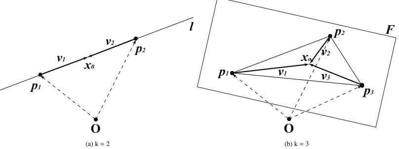
Before we analyze the optimal number of nearest neighbors for the proposed MI-MDS method with the given Pubchem dataset, I would like to mention how the proposed MI-MDS solves the mapping ambiguity problem when k=2,3 for a three dimensional target space. When the target dimension is 3D space, logically, the optimal position of the interpolated points can be in a circle if k=2, and the optimal position of the inter-polated points can be at two symmetric positions with respect to the face containing all three nearest neighbors, as in the case of

k=3. The derivative MI-MDS equation in Eq. (17), however, constrains the interpolation space corresponding to the number of nearest neighbors by setting the initial position as the aver-age of the mappings of nearest neighbors. In the case of k=2, the interpolation space is constructed as a line (l), which in-cludes the mapping positions of the two nearest neighbors when the initial mapping of the interpolation is the center of nearest neighbors ( p). Similarly, the possible mapping position of the interpolated point is constrained within the Face (F) when it contains the three nearest neighbors and k=3.

Fig. 3-(a) and -(b) illustrate the constrained interpolation space in case of k = 2 and 3, respectively. In Fig. 3, x0

O

v

v

l

p

p

x

(a) k=2

O

v

v

F

p

p

x

p

v

(b) k=3

Figure 3: The illustration of the constrained interpolation space when k=2 or k=3 by initialization at the center of the mappings of the nearest neighbors.

target dimension of nearest neighbors. Note that x0(=p) is on

the line l when k=2 and on the face F when k=3. If v1and v2

are on the same line l,αv1+βv2is also on the same line l.

Sim-ilarly, if v1, v2, and v3are on the same face F,αv1+βv2+γv3

is also on the same face F. Thus, the final mapping position of the interpolated point with k=2 or 3 is constrained in the line

l or face F, as shown in Fig. 3. This results in removing the

ambiguity of the optimal mapping position of the small nearest neighbor cases, for example k=2,3 when the target dimension is 3.

We can think of two MI-MDS specific properties as possible reasons for the results of the experiment of the optimal num-ber of nearest neighbors, which is shown in Fig. 2. A distinct feature of the MI-MDS algorithm compared to other k-NN ap-proaches is that the increase of the number of nearest neighbors results in generating a more complicated problem space to find the mapping position of the newly interpolated point. Note that the interpolation approach allows only the interpolated point to be moved and the selected nearest neighbors are fixed in the target dimension. This algorithmic property effects more se-vere constraints to find optimal mapping position with respect to Eq. (4). Also, note that finding the optimal interpolated po-sition does not guarantee that it makes better mapping in terms of full data mapping, but it means that the MI-MDS algorithm works as the algorithm designed.

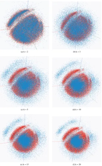
Another specific property of MI-MDS is that the purpose of the MI-MDS algorithm is to find appropriate embeddings for the new points based on the given mappings of the sample data. Thus, it could be better to be sensitive to the mappings of closely-located nearest neighbors of the new point than to be biased to the distribution of the mappings of whole sample points. Fig. 4 illustrates the mapping difference with respect to the number of nearest neighbors used for the MI-MDS al-gorithm with 50k sample and 50k out-of-sample data. The 50k sample data are selected randomly from the given 100k data set, so it is reasonable that the sampled 50k data and out-of-sample 50k show similar distributions. As shown in Fig. 4-(a), the in-terpolated points are distributed similarly to the sampled data as we expected. Also, Fig. 4-(a) is much more similar to the configuration of the full MDS running with 100k data, which

is shown later in this paper, than other results in Fig. 4. On the other hand, Fig. 4-(b) through Fig. 4-(f) are shown in center-biased mapping, and the degree of bias of those mappings in-creases as k inin-creases.

In order to understand more about why biased mappings are generated by larger nearest neighbors cases with the test dataset, we have investigated the given original distance distri-bution of the 50k sampled data set and the trained mapping dis-tance distribution of the sampled data. Also, we have analyzed the training mapping distance between k-NNs with respect to

k. Fig. 5 is the histogram of the original distance distribution

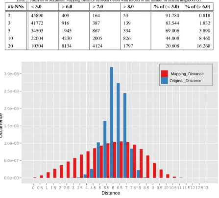
and the trained mapping distance distribution of 50k sampled data used in Fig. 2 and Fig. 4. As shown in Fig. 5, most of the original distances are between 5 and 7, but the trained map-ping distances reside in a broader interval. Table 2 demonstrates the distribution of the maximum mapping distance between se-lected k-NNs with respect to the number of nearest neighbors. The maximum original distance is 10.198 and the maximum mapping distance of the 50k sampled data is 12.960.

As shown in Fig. 18-(a), the mapping of Pubchem data forms a spherical shape. Thus, the maximum mapping distance of the 50k sampled data could be similar to the diameter of the spherical mapping. The distance 3.0 is close to half of radius of the sphere and the distance 6.0 is close to the radius of the sphere. Therefore, in Table 2 the column of “<3.0” represents the cases that nearest neighbors are closely mapped together, and the columns of “>6.0” and others illustrate the cases that some nearest neighbors are far from other nearest neighbors. Note that the entries of “>6.0” column include that of “>7.0” and “>8.0” as well.

The analysis of mapping distances between k-NNs with the tested Pubchem dataset shows interesting results. Initially, we expected that k =5 or k =10 could be small enough numbers of the nearest neighbors, which would position nearest neigh-bors near each other in the target dimension. Contrary to our expectation, as shown in Table 2, even in the case of k = 2, nearest neighbors are not near each other for some interpolated data. The cases of two nearest neighbors positioned more than a 6.0 distance occurred more than 400 times. As we increase

(a) k=2 (b) k=3

(c) k=5 (d) k=10

(e) k=15 (f) k=20

Table 2: Analysis of Maximum Mapping Distance between k-NNs with respect to the number of nearest neighbors (k).

#k-NNs <3.0 >6.0 >7.0 >8.0 % of (<3.0) % of (>6.0)

2 45890 409 164 53 91.780 0.818

3 41772 916 387 139 83.544 1.832

5 34503 1945 867 334 69.006 3.890

10 22004 4230 2005 826 44.008 8.460

20 10304 8134 4124 1797 20.608 16.268

Distance

Occurrence

0.0e+00 5.0e+07 1.0e+08 1.5e+08 2.0e+08 2.5e+08 3.0e+08

0 0.5 1 1.5 2 2.5 3 3.5 4 4.5 5 5.5 6 6.5 7 7.5 8 8.5 9 9.5 10 10.5 11 11.5 12 12.5 13

Mapping_Distance Original_Distance

Figure 5: Histogram of the original distance and the pre-mapping distance in the target dimension of 50k sampled data of 100k. The maximum original distance of the 50k sampled data is 10.198 and the maximum mapping distance of the 50k sampled data is 12.960.

nearest neighbors distanced more than 6.0 increases more than twice what it was when k = 2. On the other hand, the num-ber of the cases of all of the selected nearest neighbors closely mapped decreases in Table 2. The percentage of the cases of all selected neareset neighbors closely mapped is also shown in Table 2. Between the cases of k=2 and k=3, the difference of the all k-NNs closely mapped cases is about 8.2% of a 50k out-of-sample points. For the case of k=20, the occurrence of closely mapped cases drops from 91.8% to 20.6%.

From the above investigation of the mapping distance dis-tribution between selected nearest neighbors, it is found that, even with a small number of nearest neighbors, the neighbors can be mapped relatively far from each other, and the number of those cases is increased as k is increased. The long-distance mappings between nearest neighbors could result in generating center-biased mappings by interpolation. We can think of this as a reason for why the 2-NN case shows better results than

other cases that use the larger number of nearest neighbors with the Pubchem dataset.

In short, as we explored the optimal number of nearest neigh-bors with the Pubchem data set, k = 2 is the optimal case as shown in Fig. 2, and the larger nearest neighbor cases show biased mapping results, as shown in Fig. 4. Therefore, we use 2-NN for the forthcoming MI-MDS experimental analyses with Pubchem datasets in this section.

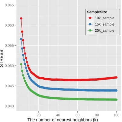
In addition, we would like to test the proposed inter-polation method with totally different dataset, which is a metagenomics sequence dataset with 30000 points (hereafter

MC30000 dataset). We generated the dissimilarity matrix based on a local sequence alignment algorithm called Smith-Waterman (SW) [22].

The number of nearest neighbors (k)

STRESS

0.040 0.045 0.050 0.055 0.060 0.065

20 40 60 80 100

SampleSize

10k_sample

15k_sample

20k_sample

Figure 6: Quality comparison between interpolated result of 30,000 with re-spect to the number of nearest neighbors (k) with various sample and out-of-sample points result.

20000 sample points, and a different number of nearest neigh-bors (k) in Fig. 6. As we expected, the more number of sample points result in the better quality of mappings by the proposed MI-MDS.

The experimental result of the optimal number of nearest neighbors with MC30000 dataset is totally opposite with the above experiments with Pubchem data set. In contrast to Fig. 2, the mapping quality with a smaller number of nearest neighbors is worse than with a larger number of nearest neighbors in Fig. 6 with all tested sample sizes. In detail, the proposed MI-MDS algorithm shows the best mapping quality of MC30000 dataset with 10000 sample points when the number of nearest neigh-bors is 57. As seen in Fig. 6, the mapping quality of MI-MDS with 10000 samples in MC30000 is similar to each other, when

k is in between 40 and around 80. In Fig. 6, the mapping

qual-ity of MI-MDS with 15000 and 20000 samples in MC30000 dataset converges when k is larger than 60.

We could deduce that the contrast results of k-NN experi-ments between pubchem and MC30000 dataset are due to the different property of input data and how to measure dissimilar-ity. For the pubchem dataset case, a dissimilarity between two points is actually a Euclidean distance between two 166-bit bi-nary feature vectors. Thus, a zero dissimilarity occurs if and only if the corresponding two points (a.k.a. two chemical com-pounds) are represented by an identical binary feature vector, and zero dissimilarity between two points means actually that the two points are essentially the same in the original space. In reality, there are only a few cases of zero dissimilarity between two different chemical compounds occur among 100000 pub-chem dataset. Also, if two different points (say point b and c) are significantly close to a point (a), then those points (b and c) are close to each other.

On the other hand, for the MC30000 dataset case,

dissimilar-ity is calculated based on SW local alignment algorithm result. A dissimilarity between two different sequences is measured based on the corresponding two subsequences of the original two different sequences, which are locally-aligned by the SW local alignment algorithm, so it is possible to have zero dissimi-larity between two different sequences when the locally-aligned two subsequences are identical. Practically, there are quite large amounts of non-diagonal zero dissimilarities exist in the given original dissimilarity matrix of the MC30000 dataset. Hence, zero dissimilarity cannot guarantee that the corresponding pair of points (or sequences) should be the same position in the orig-inal space and in the target space. For instance, although point a has zero dissimilarities with the other two points (b and c), the given dissimilarity between point b and c could be larger than zero.

Since the dissimilarity measure of pubchem data is reliable and consistent, a small number of nearest neighbors would be enough to find a mapping for an interpolated point in pubchem dataset. However, when the dissimilarity measurement is un-reliable, such as MC30000 dataset case as mentioned in the above paragraph, a large number of nearest neighbors could be required to compliment the unreliability of each dissimilarity value, as shown in Fig. 6.

5.2. Comparison between MDS and MI-MDS

Sample size

STRESS

0.00 0.02 0.04 0.06 0.08 0.10

2e+04 4e+04 6e+04 8e+04 1e+05

Algorithm

MDS

INTP

Figure 7: Quality comparison between the interpolated result of 100k with re-spect to the different sample sizes (INTP) and the 100k MDS result (MDS)

5.2.1. Fixed Full Data Case

and interpolated results with 50k is only around 0.0038. Even with a small portion of sample data (12.5k is only 1/8 of 100k), the proposed MI-MDS algorithm produces good enough map-ping in the target dimension using a much smaller amount of time than when we ran MDS with the full 100k data.

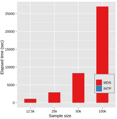
In Fig. 8, we compare the accumulated running time of the

out-of-sample approach, which combines the full MDS running

time of sample data and MI-MDS running time of the out-of-sample data with respect to different sample size, to the run-ning time of the full MDS run with the 100k data. As shown in Fig. 8, the overall running time of the out-of-sample ap-proach is much smaller than the full MDS apap-proach. To be more specific, the out-of-sample approach for the 100k dataset is around 25.1, 9.3, and 3.3 times faster than the full MDS ap-proach with respect to different sample sizes, 12.5k, 25k, and 50k, respectively.

Sample size

Elapsed time (sec)

0 5000 10000 15000 20000 25000

12.5k 25k 50k 100k

MDS

INTP

Figure 8: Running time comparison between the Out-of-Sample approach, which combines the full MDS running time with sample data and the MI-MDS running time with out-of-sample data when N =100k with respect to the dif-ferent sample sizes and the full MDS result of the 100k data.

Fig. 9 shows the MI-MDS interpolation running time only with respect to the sample data using 16 nodes of the Cluster-II in Table 1. The MI-MDS algorithm takes around 8.55, 14.35, and 18.98 seconds with different sample sizes, i.e. 12.5k, 25k, and 50k, to find new mappings of 87500, 75000, and 50000 points based on the pre-mapping results of the corresponding sample data. In Fig. 9 we find the interesting feature that it takes much less time to find new mappings of 87,500 points (8.55 seconds) than to find new mappings of 50,000 points (18.98 seconds). The reason for this is that the computational time complexity of the MI-MDS is O(Mn) where n is the sample size and M=N−n. Thus, the running time of MI-MDS is

pro-portional to the number of new mapping points if the sample size (n) is the same, as in the larger data set case shown below in this paper. However, the above case is the opposite case. The full data size (N) is fixed, so that both the sample data size (n) and the out-of-sample data size (M) are variable and correlated.

We can illustrateO(Mn) as a simple quadratic equation of vari-able n as following: O(n∗(N−n)) = O(N ∗n−n2_{), which}

has a maximum when n = N/2. The above experiment case

N =100k and n =50k is the maximum case, so that the case of 50k sample data of MI-MDS took longer than the case of the 12.5k sample data.

Sample size

Elapsed time (sec)

0 5 10 15 20

12.5k 25k 50k

Algorithm

INTP

Figure 9: Elapsed time of parallel MI-MDS running time of 100k data with respect to the sample size using 16 nodes of the Cluster-II in Table 1. Note that the computational time complexity of MI-MDS isO(Mn) where n is the sample size and M=N−n.

In addition to experiment on pubchem dataset, we also in-vestigated the MI-MDS result with MC30000 dataset. Fig. 10 depicts the mapping quality comparison between the full MDS result of the MC30000 and the MI-MDS results of MC30000 dataset with different sample sizes. The mapping quality of the proposed MI-MDS method with different sample size in Fig. 10 is the result of the best k-NN case of Fig. 6. As similar as in Fig. 7, the mapping quality of the MC30000 dataset by the MI-MDS is getting better as the sample size increases. The difference of the normalized STRESS value between a full MDS result and the MI-MDS result with 20000 sample for the MC30000 dataset is only around 0.00468.

5.2.2. Fixed Sample Data Size

Sample size

STRESS

0.00 0.02 0.04 0.06 0.08 0.10

10000 15000 20000 25000 30000

Algorithm

MDS

INTP

Figure 10: Quality comparison between the interpolated results of 30000 Metagenomics sequence dataset with respect to the different sample sizes (INTP) and the full MDS result (MDS)

Table 3: Large-scale MI-MDS running time (seconds) with 100k sample data

1 Million 2 Million 4 Million

731.1567 1449.1683 2895.3414

based on that 100k mapping; they have about a 0.007 diff er-ence in the normalized STRESS criteria. However, there is not much difference between the normalized STRESS values of the 1M, 2M, and 4M interpolated results, although the sample size is quite a small portion of the total data and the out-of-sample data size increases up to four times larger size. From the above results we could consider that the proposed MI-MDS algorithm works well and is scalable if we are given a good enough pre-configured result that represents the structure of the given data well. Note that it is not possible to run the SMACOF algorithm with only 200k data points due to memory bounds within the systems in Table 1.

We also measure the runtime of the MI-MDS algorithm with a large-scale data set up to 4 million points. Fig. 12 shows the running time of the out-of-sample approach in an accumu-lated bar graph, which represents the full MDS running time of sample data (M =100k) in the red bar and the MI-MDS in-terpolation time of out-of-sample data (n =1M, 2M, and 4M) in the blue bar on top of the red bar. As we expected, the run-ning time of MI-MDS is much faster than the full MDS runrun-ning time in Fig. 12. Although the MI-MDS interpolation running time in Table 3 is much smaller than the full MDS running time (27006 seconds), the MI-MDS deals with a much larger amount of points, i.e. 10, 20, and 40 times larger. Although we can-not run the parallel SMACOF algorithm [7] with even 200,000 points on our current sytsems in Table 1, if we assume that we are able to run the parallel SMACOF algorithm with millions of points on Cluster-II in Table 1, then the parallel SMACOF will

Total size

STRESS

0.00 0.02 0.04 0.06 0.08 0.10

1e+06 2e+06 3e+06 4e+06

Figure 11: The STRESS value change of the interpolation larger data, such as 1M, 2M, and 4M data points, with 100k sample data. The initial STRESS value of MDS result of 100k data is 0.0719.

Total size

Elapsed time (sec)

0 5000 10000 15000 20000 25000

100k 100k+1M 100k+2M 100k+4M MDS INTP

Figure 12: Running time of the Out-of-Sample approach, which combines the full MDS running time with sample data (M=100k) and the MI-MDS running time with different out-of-sample data sizes, i.e. 1M, 2M, and 4M.

take 100, 400, and 1600 times longer with 1M, 2M, and 4M data than the running time of the parallel SMACOF with 100k data, due to theO(N2_{) computational complexity. As opposed}

to the approximated full MDS running time, the proposed MI-MDS interpolation takes much less time to deal with millions of points than the parallel SMACOF algorithm. In numeric terms, MI-MDS interpolation is around 3693.5, 7454.2, and 14923.8 times faster than approximated full parallel MDS running time with 1M, 2M, and 4M data, respectively.

should be proportional to the number of out-of-sample data since the sample data size is fixed. Table 3 shows the exact running time of the MI-MDS interpolation method with respect to the number of the out-of-sample data size (n), based on the same sample data (M =100k). The running time is almost ex-actly proportional to the out-of-sample data size (n), which is as it should be.

5.3. Parallel Performance Analysis of MI-MDS

In the above section we discussed the quality of the con-structed configuration of the MI-MDS approach based on the STRESS value of the interpolated configuration, and the run-ning time benefits of the proposed MI-MDS interpolation ap-proach. Here, we would like to investigate the MPI communi-cation overhead and parallel performance of the proposed par-allel MI-MDS implementation in Section 4.1 in terms of effi -ciency with respect to the running results within Cluster-I and Cluster-II in Table 1.

First of all, we prefer to investigate the parallel overhead, especially the MPI communication overhead, which could be significant for the parallel MI-MDS in Section 4.1. Parallel MI-MDS consists of two different computations, the interpo-lation part and the STRESS calcuinterpo-lation part. The interpointerpo-lation part is pleasingly parallel and its computational complexity is O(M), where M=N−n, if the sample size n is considered as a

constant. The interpolation part uses only two MPI primitives,

MPI_GATHERandMPI_BROADCAST, at the end of interpolation to gather all the interpolated mapping results and spread out the combined interpolated mapping results to all the processes for further computation. Thus, the communicated message amount through MPI primitives isO(M), so it is not dependent on the number of processes but the number of whole out-of-sample points.

For the STRESS calculation, which was applied to the pro-posed symmetric pairwise computation in Section 4.2, each process usesMPI_SENDRECVk times to send an assigned block

or rolled block whose size is M/p, where k =⌈(p−1)/2⌉for communicating required data andMPI_REDUCEtwice for calcu-latingPi<j(di j−δi j)2andPi<jδ2i j. Thus, the MPI communicated

data size isO(M/p×p)=O(M) without regard to the number of processes.

The MPI overhead during the interpolation and the STRESS calculating at Cluster-I and Cluster-II in Table 1 are shown in Fig. 13 and Fig. 14, respectively. Note that the x-axis of both figures is the sample size (n) but not M =N−n. In the figures

the model is generated asO(M) starting with the smallest sam-ple size – here 12.5k. Both Fig. 13 and Fig. 14 show that the actual overhead measurement follows the MPI communication overhead model.

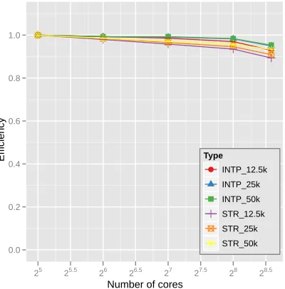
Fig. 15 and Fig. 16 illustrate the efficiency of the interpola-tion and the STRESS calculainterpola-tion of the parallel MI-MDS run-ning results with different sample sizes – 12.5k, 25k, and 50k – with respect to the number of parallel units using Cluster-I and Cluster-II, respectively. Equations for efficiency follow:

Sample size

MPI o

v

erhead time (sec)

0.5 1.0 1.5 2.0 2.5

15000 20000 25000 30000 35000 40000 45000 50000 Type

INTP_model

INTP_Ovhd

STR_model

STR_Ovhd

Figure 13: Parallel overhead modeled from MPI communication in terms of sample data size (m) using Cluster-I in Table 1 and message passing overhead model.

Sample size

MPI o

v

erhead time (sec)

0.4 0.6 0.8 1.0

15000 20000 25000 30000 35000 40000 45000 50000 Type

INTP_model

INTP_Ovhd

STR_model

STR_Ovhd

Figure 14: Parallel overhead modeled from MPI communication in terms of sample data size (m) using Cluster-II in Table 1 and message passing overhead model.

f = pT (p)−T (1)

T (1) (20)

ε= 1

1+f (21)

where p is the number of parallel units, T (p) is the running time with p parallel units, and T (1) is the sequential running time. In practice, Eq. (20) can be replaced with the following:

f =αT (p1)−T (p2)

whereα = p1/p2and p2is the smallest number of used cores

for the experiment, so alpha ≥ 1. We use Eq. (22) for the overhead calculation.

Number of cores

Efficiency

0.0 0.2 0.4 0.6 0.8 1.0

24 24.5 25 25.5 26 26.5 27 Type

INTP_12.5k

INTP_25k

INTP_50k

STR_12.5k

STR_25k

STR_50k

Figure 15: Efficiency of the interpolation part (INTP) and the STRESS evalu-ation part (STR) runtimes in the parallel MI-MDS applicevalu-ation with respect to different sample data sizes using Cluster-I in Table 1. The total data size is 100k.

Number of cores

Efficiency

0.0 0.2 0.4 0.6 0.8 1.0

25 25.5 26 26.5 27 27.5 28 28.5 Type

INTP_12.5k

INTP_25k

INTP_50k

STR_12.5k

STR_25k

STR_50k

Figure 16: Efficiency of the interpolation part (INTP) and the STRESS evalu-ation part (STR) runtimes in the parallel MI-MDS applicevalu-ation with respect to different sample data sizes using Cluster-II in Table 1. The total data size is 100k.

In Fig. 15, 16 to 128 cores are used to measure parallel per-formance with 8 processes, and 32 to 384 cores are used to evaluate the parallel performance of the proposed parallel MI-MDS with 16 processes in Fig. 16. Processes communicate via MPI primitives and each process is also parallelized at the thread level. Both Fig. 15 and Fig. 16 show very good efficiency

with an appropriate degree of parallelism. Since both the inter-polation part and the STRESS calcualtion part are pleasingly parallel within a process, the major overhead portion is the MPI message communication overhead unless load balance is not achieved in the thread-level parallelization within each process. In the previous paragraphs, the MPI communicating over-head is investigated and the MPI communication overover-head showsO(M) relation. Thus, the MPI overhead is constant if we examine it with the same number of processes and the same out-of-sample data sizes. Since the parallel computation time decreases as more cores are used, but the overhead time re-mains constant, this property lowers the efficiency as the num-ber of cores is increased, as we expected. Note that the numnum-ber of processes that lowers the efficiency dramatically is different from Cluster-I to Cluster-II. The reason for this is that the MPI overhead time of Cluster-I is bigger than that of Cluster-II due to different network environments, i.e. Giga bit ethernet and 20Gbps Infiniband. The difference is easily found by compar-ing Fig. 13 and Fig. 14.

5.4. Large-Scale Data Visualization via MI-MDS

Fig. 17 shows the proposed MI-MDS results of a 100k Pub-Chem dataset with respect to the different sample sizes, such as (a) 12.5k and (b) 50k. Sampled data and interpolated points are colored in red and blue, respectively. We have also processed a large volume of PubChem data with our parallel interpolation algorithms for MDS by using our Cluster-II, and the results are shown in Fig. 18. We performed parallel MI-MDS to process datasets from hundreds of thousand up to 4 million by using the 100k PubChem data set as a training set. In Fig. 18 we show the MI-MDS result of a 2 million point dataset based on a 100k point training set, compared to the mapping of 100k training set data. The interpolated points are colored in blue, while the training points are in red. As one can see, our interpolation algorithms have produced a map closest to the training dataset.

6. Conclusion and Future Work

In this paper we have proposed interpolation algorithms for extending the MDS dimension reduction approaches to very large datasets into the millions. The proposed interpolation approach consists of two-phases: (1) the full MDS running with sampled data (n); and (2) the interpolation of out-of-sample data (N−n) based on the mapped position of sampled

data. The proposed interpolation algorithm reduces the com-putational complexity of the MDS algorithm from O(N2_{) to}

O(n×(N−n)). The iterative majorization method is used as an

optimization method for finding mapping positions of the inter-polated point. We have also proposed in this paper the usage of parallelized interpolation algorithms for MDS, which can uti-lize multicore/multiprocessor technologies. In particular, we utilized a simple but highly efficient mechanism for computing the symmetric all-pairwise distances to provide improved per-formance.

(a) MDS 12.5k (b) MDS 50k

Figure 17: Interpolated MDS results of the total 100k PubChem dataset trained by (a) 12.5k and (b) 50k sampled data. Sampled data are colored in red and interpolated points are in blue.

(a) MDS 100k (trained set) (b) MDS 2M+100k

Figure 18: Interpolated MDS results. Based on 100k samples (a), additional 2M PubChem dataset is interpolated (b). Sampled data are colored in red and interpolated points are in blue.

number of k-NN. 2-NN is the best case for the Pubchem data, which we used as a test dataset in this paper. We have shown that our interpolation approach gives results of good quality with high parallel performance. In a quality comparison the ex-perimental results show that the interpolation approach output is comparable to the normal MDS output, while taking much less running time and requiring much less memory than the normal MDS methods. The proposed interpolation algorithm is easy to parallelize since each interpolated point is indepen-dent of the other out-of-sample points, so many points can be interpolated concurrently without communication. The parallel

performance is analyzed in Section 5.3, and it shows very high efficiency as we expected.

the Cluster-II system, it would take around 15,000 times longer than the interpolation approach as mentioned in Section 5.2.

Future research could be the application of these ideas to dif-ferent areas including metagenomics and other DNA sequence visualization. Also, we are working on how to reduce the qual-ity gap between the normal MDS methods and the MDS inter-polating method.

References

[1] G. Fox, S. Bae, J. Ekanayake, X. Qiu, H. Yuan, Parallel Data Mining from Multicore to Cloudy Grids, in: Proceedings of HPC 2008 High Per-formance Computing and Grids workshop, Cetraro, Italy, 2008. [2] C. Bishop, M. Svens´en, C. Williams, GTM: A Principled Alternative to

the Self-Organizing Map, Advances in Neural Information Processing Systems (1997) 354–360.

[3] C. Bishop, M. Svens´en, C. Williams, GTM: The Generative Topographic Mapping, Neural Computation 10 (1) (1998) 215–234.

[4] T. Kohonen, The Self-Organizing Map, Neurocomputing 21 (1-3) (1998) 1–6.

[5] J. B. Kruskal, M. Wish, Multidimensional Scaling, Sage Publications Inc., Beverly Hills, CA, U.S.A., 1978.

[6] I. Borg, P. J. Groenen, Modern Multidimensional Scaling: Theory and Applications, Springer, New York, NY, U.S.A., 2005.

[7] J. Y. Choi, S.-H. Bae, X. Qiu, G. Fox, High Performance Dimension Re-duction and Visualization for Large High-dimensional Data Analysis, in: Proceedings of the 10th IEEE/ACM International Symposium on Cluster, Cloud and Grid Computing (CCGRID) 2010, 2010, pp. 331–340. [8] S.-H. Bae, J. Y. Choi, X. Qiu, G. Fox, Dimension Reduction and

Visu-alization of Large High-dimensional Data via Interpolation, in: Proceed-ings of the 19th ACM International Symposium on High Performance Distributed Computing (HPDC) 2010, Chicago, Illinois, 2010, pp. 203– 214.

[9] Z. Wang, S. Zheng, Y. Ye, S. Boyd, Further Relaxations of the Semidefinite Programming Approach to Sensor Network

Lo-calization, SIAM Journal on Optimization 19 (2) (2008) 655–673. doi:http://dx.doi.org/10.1137/060669395.

[10] Y. Bengio, J.-F. Paiement, P. Vincent, O. Delalleau, N. L. Roux, M. Ouimet, Out-of-Sample Extensions for LLE, Isomap, MDS, Eigen-maps, and Spectral Clustering, in: Advances in Neural Information Pro-cessing Systems, MIT Press, 2004, pp. 177–184.

[11] M. W. Trosset, C. E. Priebe, The Out-of-Sample Prob-lem for Classical Multidimensional Scaling, Computational Statistics and Data Analysis 52 (10) (2008) 4635–4642. doi:http://dx.doi.org/10.1016/j.csda.2008.02.031.

[12] W. S. Torgerson, Multidimensional scaling: I. Theory and method, Psy-chometrika 17 (4) (1952) 401–419.

[13] S. Ingram, T. Munzner, M. Olano, Glimmer: Multilevel MDS on the GPU, IEEE Transactions on Visualization and Computer Graphics 15 (2) (2009) 249–261.

[14] J. B. Kruskal, Multidimensional Scaling by Optimizing Goodness of Fit to a Nonmetric Hypothesis, Psychometrika 29 (1) (1964) 1–27. [15] Y. Takane, F. W. Young, J. de Leeuw, Nonmetric Individual Differences

Multidimensional Scaling: an Alternating Least Squares Method with Optimal Scaling Features, Psychometrika 42 (1) (1977) 7–67.

[16] J. de Leeuw, Applications of Convex Analysis to Multidimensional Scal-ing, Recent Developments in Statistics (1977) 133–145.

[17] J. de Leeuw, Convergence of the Majorization Method for Multidimen-sional Scaling, Journal of Classification 5 (2) (1988) 163–180.

[18] A. Dempster, N. Laird, D. Rubin, Maximum Likelihood from Incomplete Data via the EM Algorithm, Journal of the Royal Statistical Society. Se-ries B (1977) 1–38.

[19] T. M. Cover, P. E. Hart, Nearest Neighbor Pattern Classification, IEEE Transaction on Information Theory 13 (1) (1967) 21–27.

[20] J. Qiu, S. Beason, S. Bae, S. Ekanayake, G. Fox, Performance of Win-dows Multicore Systems on Threading and MPI, in: Proceedings of 10th IEEE/ACM International Conference on Cluster, Cloud and Grid Com-puting, IEEE, 2010, pp. 814–819.

[21] R. Kohavi, A Study of Cross-Validation and Bootstrap for Accuracy Esti-mation and Model Selection, in: International Joint Conference on Artifi-cial Intelligence, Vol. 14, Morgan Kaufmann, 1995, pp. 1137–1145. [22] T. F. Smith, M. S. Waterman, Identification of Common Molecular