This is a single-user version of this eBook.
It may not be copied or distributed.
Unauthorized reproduction or distribution of this eBook
Telecommunications
Demystified
A Streamlined Course in Digital Communications
(and some Analog) for EE Students and
Practicing Engineers
by Carl Nassar
All rights reserved. No part of this book may be reproduced, in any
form or means whatsoever, without written permission of the
pub-lisher. While every precaution has been taken in the preparation of
this book, the publisher and author assume no responsibility for errors
or omissions. Neither is any liability assumed for damages resulting
from the use of information contained herein.
Printed in the United States of America.
ISBN 1-878707-77-9 (eBook)
iii
Contents
Foreword xv
What’s on the CD-ROM? xvii
CHAPTER 1
Introducing Telecommunications ... 1
1.1 Communication Systems ... 1
1.1.1 Definition ... 1
1.1.2 The Parts of a Communication System ... 2
1.1.3 An Example of a Communication System ... 2
1.2 Telecommunication Systems ... 3
1.2.1 Definition ... 3
1.2.2 Four Examples and an Erratic History Lesson ... 4
1.3 Analog and Digital Communication Systems ... 6
1.3.1 Some Introductory Definitions ... 6
1.3.2 Definitions ... 7
1.3.3 And Digital Became the Favorite ... 8
1.3.4 Making It Digital ... 9
1.4 Congrats and Conclusions ... 10
CHAPTER 2
Telecommunication Networks ... 13
2.1 Telecommunication Network Basics ... 13
2.1.1 Connecting People with Telephones ... 13
2.1.2 Connecting More People, Farther Apart ... 14
2.1.3 Multiplexing—An Alternative to a Lot of Wire ... 16
iv
2.2 POTS: Plain Old Telephone System ... 19
2.2.1 Local Calls ... 19
2.2.2 Long Distance Calls ... 20
2.2.3 The Signals Sent from Switching Center to Switching Center ... 21
2.3 Communication Channels ... 24
2.3.1 Transmission Lines (Wires) ... 24
2.3.2 Terrestrial Microwave ... 26
2.3.3 Satellite Connections ... 28
2.3.4 Fiber-optic Links ... 29
2.4 Data Communication Networks ... 31
2.5 Mobile Communications ... 33
2.6 Local Area Networks (LANs) ... 35
2.7 Conclusion ... 37
CHAPTER 3
A Review of Some Important Math, Stats, and Systems ... 39
3.1 Random Variables ... 39
3.1.1 Definitions ... 39
3.1.2 The Distribution Function: One Way to Describe x ... 39
3.1.3 The Density Function: A Second Way to Describe x ... 40
3.1.4 The Mean and the Variance ... 41
3.1.5 Multiple Random Variables ... 44
3.2 Random Processes ... 45
3.2.1 A Definition ... 45
3.2.2 Expressing Yourself, or a Complete Statistical Description .. 47
3.2.3 Expressing Some of Yourself, or a Partial Description ... 47
3.2.4 And in Telecommunications … ... 48
3.3 Signals and Systems: A Quick Peek ... 50
3.3.1 A Few Signals ... 50
3.3.2 Another Way to Represent a Signal: The Fourier Transform ... 51
3.3.3 Bandwidth ... 53
3.3.4 A Linear Time Invariant (LTI) System ... 55
3.3.5 Some Special Linear Time Invariant (LTI) Systems ... 56
v
CHAPTER 4
Source Coding and Decoding: Making it Digital ... 61
4.1 Sampling ... 61
4.1.1 Ideal Sampling ... 61
4.1.2 Zero-order Hold Sampling ... 67
4.1.3 Natural Sampling ... 69
4.2 Quantization ... 71
4.2.1 Meet the Quantizer ... 71
4.2.2 The Good Quantizer ... 77
4.2.3 The Quantizer and the Telephone ... 88
4.3 Source Coding: Pulse Code Modulator (PCM) ... 92
4.3.1 Introducing the PCM ... 92
4.3.2 PCM Talk ... 93
4.3.3 The “Good” PCM... 94
4.3.4 Source Decoder: PCM Decoder ... 95
4.4 Predictive Coding ... 96
4.4.1 The Idea Behind Predictive Coding ... 97
4.4.2 Why? ... 97
4.4.3 The Predicted Value and the Predictive Decoder ... 98
4.4.4 The Delta Modulator (DM) ... 99
4.4.5 The Signals in the DM ... 101
4.4.6 Overload and Granular Noise ... 105
4.4.7 Differential PCM (DPCM) ... 107
4.5 Congrats and Conclusion ... 110
CHAPTER 5
Getting It from Here to There: Modulators and Demodulators ... 115
5.1 An Introduction ... 115
5.2 Modulators ... 116
5.2.1 Baseband Modulators ... 116
5.2.2 Bandpass Modulators ... 124
5.3 Just-in-Time Math, or How to Make a Modulator Signal Look Funny ... 133
5.3.1 The Idea ... 134
vi
5.4.1 What Demodulators Do ... 146
5.4.2 The Channel and Its Noise ... 147
5.4.3 Building a Demodulator, Part I—the Receiver Front End ... 148
5.4.4 The Rest of the Demodulator, Part II—The Decision Makers ... 152
5.4.5 How to Build It ... 156
5.5 How Good Is It Anyway (Performance Measures) ... 161
5.5.1 A Performance Measure ... 161
5.5.2 Evaluation of
P( )
ε
for Simple Cases ... 1625.5.3 Some well-known
P( )
ε
’s ... 1665.6 What We Just Did ... 166
CHAPTER 6
Channel Coding and Decoding: Part 1–Block Coding and Decoding ... 171
6.1 Simple Block Coding ... 172
6.1.1 The Single Parity Check Bit Coder ... 172
6.1.2 Some Terminology ... 175
6.1.3 Rectangular Codes ... 175
6.2 Linear block codes ... 177
6.2.1 Introduction ... 177
6.2.2 Understanding Why ... 179
6.2.3 Systematic Linear Block Codes ... 181
6.2.4 The Decoding ... 182
6.3 Performance of the Block Coders ... 188
6.3.1 Performances of Single Parity Check Bit Coders/Decoders ... 188
6.3.2 The Performance of Rectangular Codes ... 189
6.3.3 The Performance of Linear Block Codes ... 189
6.4 Benefits and Costs of Block Coders ... 192
vii
Channel Coding and Decoding:
Part 2–Convolutional Coding and Decoding ... 197
7.1 Convolutional Coders ... 197
7.1.1 Our Example ... 197
7.1.2 Making Sure We’ve Got It ... 199
7.1.3 Polynomial Representation ... 200
7.1.4 The Trellis Diagram ... 201
7.2 Channel Decoding ... 203
7.2.1 Using a Trellis Diagram ... 204
7.2.2 The Viterbi Algorithm ... 206
7.3 Performance of the Convolutional Coder ... 213
7.4 Catastrophic Codes ... 214
7.5 Building Your Own ... 216
CHAPTER 8
Trellis-Coded Modulation (TCM)
The Wisdom of Modulator and Coder Togetherness ... 221
8.1 The Idea ... 222
8.2 Improving on the Idea ... 225
8.3 The Receiver End of Things ... 230
8.3.1 The Input ... 231
8.3.2 The TCM Decoder Front End ... 233
8.3.3 The Rest of the TCM Decoder ... 234
8.3.4 Searching for the Best Path ... 237
CHAPTER 9
Channel Filtering and Equalizers ... 245
9.1 Modulators and Pulse Shaping ... 245
9.2 The Channel That Thought It Was a Filter ... 249
9.3 Receivers: A First Try ... 251
9.3.1 The Proposed Receiver ... 251
9.3.2 Making the Receiver a Good One ... 254
9.3.3 The Proposed Receiver: Problems and Usefulness ... 256
viii
9.5.1 The Input ... 262
9.5.2 A Problem with the Input, and a Solution ... 264
9.5.3 The Final Part of the Optimal Receiver ... 265
9.5.4 An Issue with Using the Whitening Filter and MLSE ... 271
9.6 Linear Equalizers ... 271
9.6.1 Zero Forcing Linear Equalizer ... 272
9.6.2 MMSE (Minimum Mean Squared Error) Equalizer ... 273
9.7 Other Equalizers: the FSE and the DFE ... 274
9.8 Conclusion ... 275
CHAPTER 10
Estimation and Synchronization ... 279
10.1 Introduction ... 279
10.2 Estimation ... 280
10.2.1 Our Goal ... 280
10.2.2 What We Need to Get an Estimate of a Given r ... 281
10.2.3 Estimating a Given r, the First Way ... 281
10.2.4 Estimating a Given r, the Second Way ... 282
10.2.5 Estimating a Given r, the Third Way ... 283
10.3 Evaluating Channel Phase: A Practical Example ... 285
10.3.1 Our Example and Its Theoretically Computed Estimate .. 285
10.3.2 The Practical Estimator: the PLL ... 290
10.3.3 Updates to the Practical Estimator in MPSK ... 292
10.4 Conclusion ... 294
CHAPTER 11
Multiple Access Schemes:
Teaching Telecommunications Systems to Share ... 299
11.1 What It Is ... 299
11.2 The Underlying Ideas ... 300
11.3 TDMA ... 303
11.4 FDMA ... 305
11.5 CDMA ... 306
11.5.1 Introduction ... 306
ix
11.5.4 MC-CDMA ... 313
11.6 CIMA ... 315
11.7 Conclusion ... 318
CHAPTER 12
Analog Communications ... 321
12.1 Modulation—An Overview ... 321
12.2 Amplitude Modulation (AM) ... 322
12.2.1 AM Modulators—in Time ... 323
12.2.2 AM Modulation—in Frequency ... 326
12.2.3 Demodulation of AM Signals—Noise-Free Case ... 328
12.2.4 An Alternative to AM—DSB-SC ... 330
12.3 Frequency Modulation (FM) ... 334
12.3.1 The Modulator in FM ... 335
12.3.2 The Demodulator in FM ... 339
12.4 The Superheterodyne Receiver ... 339
12.5 Summary ... 341
Annotated References and Bibliography ... 345
xi
Acknowledgments
In this life of mine, I have been blessed with an abundance of
won-derful people. This book would be incomplete without at least a page to
say “thank you,” for these are people alive in me and, therefore, alive in
the pages of this book.
Dr. Reza Soleymani, your careful guidance through the turmoil that
surrounded my Ph.D. days was nothing short of a miracle. You showed
me, through your example, how to handle even the most difficult of
situations with grace and grit, both academically and in all of life.
Dr. Derek Lile, Department Head at CSU—a young faculty could
not ask for better guidance. Your thoughtfulness, caring, and gentle
support have helped nurture the best of who I am. I am grateful.
Steve Shattil, Vice President of Idris Communications, you are indeed
a genius of a man whose ideas have inspired me to walk down new roads
in the wireless world. Arnold Alagar, President of Idris, thank you for
sharing the bigger picture with me, helping guide my research out of
obscure journals and into a world full of opportunity. To both of you, I am
grateful for both our technological partnerships and our friendships.
Bala Natarajan and Zhiqiang Wu, my two long-time Ph.D. students,
your support for my research efforts, through your commitment and
dedication, has not gone unnoticed. Thank you for giving so fully of
yourselves.
Dr. Maier Blostien, who asked me to change my acknowledgments
page in my Ph.D. thesis to something less gushy, let me thank you now
for saving the day when my Ph.D. days looked numbered. I appreciate
your candor and your daring.
Carol Lewis, my publisher at LLH Technology Publishing, thank
you for believing in this project and moving it from manuscript to
“masterpiece.”
xii
me the best of who you are, Mom (Mona), Dad (Rudy), and Christine
(sister)—your love has shaped me and has made this book a possibility.
Wow!
xiii
About the Author
Carl R. Nassar, Ph.D., is an engineering professor
at Colorado State University, teaching
telecommu-nications in his trademark entertaining style. He is
also the director of the RAWCom (Research in
Advanced Wireless Communications) Laboratory,
where he and his graduate students carry out
research to advance the art and science of wireless
telecommunications. In addition, he is the founder
of the Miracle Center, an organization fostering personal growth for
individuals and corporations.
Since Carl’s undergraduate and graduate school days at McGill
University, he has dreamed of creating a plain-English engineering text
with “personality.” This book is that dream realized.
To contact the author, please write or e-mail him at
xv
Foreword
I first met the author of this book, Professor Carl Nassar, after he
presented a paper at a conference on advanced radio technology.
Pro-fessor Nassar’s presentation that day was particularly informative and
his enthusiasm for the subject matter was evident. He seemed especially
gifted in terms of his ability to explain complex concepts in a clear way
that appealed to my intuition.
Some time later, his editor asked me if I would be interested in
reviewing a few chapters of this book and preparing a short preface. I
agreed to do so because, in part, I was curious whether or not his
acces-sible presentation style carried over into his writing. I was not
disappointed.
As you will soon see as you browse through these pages, Professor
Nassar does have an uncanny ability to demystify the complexities of
telecommunications systems engineering. He does so by first providing
for an intuitive understanding of the subject at hand and then, building
on that sound foundation, delving into the associated mathematical
descriptions.
I am partial to such an approach for at least two reasons. First, it has
been my experience that engineers who combine a strong intuitive
under-standing of the technology with mathematical rigor are among the best in
the field. Second, and more specific to the topic of this book, because of
the increased importance of telecommunications to our economic and
social well-being, we need to encourage students and practicing engineers
to enter and maintain their skills in the field. Making the requisite
techni-cal knowledge accessible is an important step in that direction.
In short, this book is an important and timely contribution to the
telecommunications engineering field.
Dale N. Hatfield
xvii
What’s on the CD-ROM?
The CD-ROM accompanying this book contains a fully searchable,
electronic version (eBook) of the entire contents of this book, in Adobe
®pdf format. In addition, it contains interactive MATLAB
®tutorials that
demonstrate some of the concepts covered in the book. In order to run
these tutorials from the CD-ROM, you must have MATLAB installed on
your computer. MATLAB, published by The MathWorks, Inc., is a
powerful mathematics software package used almost universally by the
engineering departments of colleges and universities, and at many
companies as well. A reasonably priced student version of MATLAB is
available from www.mathworks.com. A link to their web site has been
provided on the CD-ROM.
Using the Tutorials
Each tutorial delves deeper into a particular topic dealt with in the
book, providing more visuals and interaction with the concepts
pre-sented. Note that the explanatory text box that overlays the visuals can
be dragged to the side so that you can view the graphics and other aids
before clicking “OK” to move to the next window. Each tutorial
filename reflects the chapter in the book with which it is associated. I
recommend that you read the chapter first, then run the associated
tutorial(s) to help deepen your understanding. To run a particular
tuto-rial, open MATLAB and choose Run Script from the Command Window
File menu. When prompted, locate the desired tutorial on the CD-ROM
using the Browse feature and click “OK.” The tutorials contain basic
descriptions and text to help you use them. Brief descriptions are also
given in the following pages.
xviii
Demonstrates the creation of the DS-1 signal.
ch4_1.m
Shows the different sampling techniques, and the effects of sampling
at above and below the Nyquist rate.
ch4_2.m
Demonstrates quantization, and computation of the MSE.
ch4_3.m
Explains the operation of the DM.
ch5_1.m
Shows the workings of modulation techniques such as BPSK and
BFSK.
ch5_2.m
Explains how three signals are represented by two orthonormal basis
functions.
ch5_3.m
Illustrates the damaging effect of noise and the operation of decision
devices.
ch5_4.m
Demonstrates the performance curve for BPSK signals.
ch7.m
xix
Provides an example of how TCM works at the coder and the
decoder side.
ch9_1.m
Demonstrates how the sinc and raised cosine pulse shapes avoid ISI.
ch9_2.m
Shows how the decision device operates in the optimal receiver.
ch11.m
Provides colorful examples of TDMA, FDMA, MC-CDMA,
DS-CDMA, and CIMA.
ch12.m
Illustrates the different analog modulation techniques.
Please note that the other files on the CD-ROM are subroutines that
are called by the above-named files. You won’t want to run them on
their own, but you will need them to run these tutorials.
For MATLAB product information, please contact:
The MathWorks, Inc.
3 Apple Hill Drive
Natick, MA, 01760-2098 USA
Tel: 508-647-7000
Fax: 508-647-7101
1
Introducing
Telecommunications
I
can still recall sitting in my first class on telecommunications as anundergrad—the teacher going off into a world of technical detail and I in my chair wondering, “What is this stuff called communications and telecommunications?” So, first, some simple definitions and examples—the big picture.
1.1 Communication Systems
1.1.1 Definition
A communication system is, simply, any system in which information is transmitted from one physical location—let’s call it A—to a second physical location, which we’ll call B. I’ve shown this in Figure 1.1. A simple example of a communication system is one person talking to another person at lunch. Another simple example is one person talking to a second person over the telephone.
1.1.2 The Parts of a Communication System
Any communication system is made up of three parts, shown in Figure 1.2. First is the transmitter, the part of the communication system that sits at point A. It includes two items: the source of the information, and the technology that sends the information out over the channel. Next is the channel. The channel is the medium (the stuff) that the information travels through in going from point A to point B. An example of a channel is copper wire, or the atmosphere. Finally, there’s the receiver, the part of the commu-nication system that sits at point B and gets all the information that the transmitter sends over the channel.
We’ll spend the rest of this book talking about these three parts and how they work.
1.1.3 An Example of a Communication System
Now, let’s run through a simple but very important example of a communication system. We’ll consider the example of Gretchen talking to Carl about where to go for lunch, as shown in Figure 1.3.
TRANSMITTER RECEIVER
CHANNEL
A B
Figure 1.2 Parts of a communication system
Figure 1.3
Gretchen talking to Carl at lunch
Channel (the air)
Windpipe
The Transmitter
The transmitter, in this case, is made up of parts of Gretchen, namely her vocal cords, windpipe, and mouth. When Gretchen wants to talk, her brain tells her vocal cords (found in her windpipe) to vibrate at between 100 Hz and 10,000 Hz, depending on the sound she’s trying to make. (Isn’t it cool that, every time you talk, a part of you is shaking at between 100 and 10,000 times per second?) Once Gretchen’s vocal cords begin to vibrate, here are the three things that happen next:
(1) the vibrations of her vocal cords cause vibrations in the air in her windpipe;
(2) these vibrations in the air move up her windpipe to her mouth; and
(3) as the vibrating air moves out through Gretchen’s mouth, the shape of her mouth and lips, and the position of her tongue, work together to create the intended sound.
The Channel
In our example, the channel is simply the air between Gretchen and Carl. The shaped vibrations that leave Gretchen’s mouth cause vibrations in the air, and these vibrations move through the air from Gretchen to Carl.
The Receiver
The receiver in this case is Carl’s eardrum and brain. The vibrations in the air hit Carl’s eardrum, causing it to vibrate in the same way. Carl’s shaking eardrum sends electrical signals to his brain, which interprets the shaking as spoken sound.
The human eardrum can actually pick up vibrations between 50 Hz and 16,500 Hz, allowing us to hear sounds beyond the range of what we can speak, including a variety of musical sounds.
1.2 Telecommunication Systems
1.2.1 Definition
1.2.2 Four Examples and an Erratic History Lesson
Here are four examples of telecommunication systems, ordered chronologically to create what we’ll optimistically call “a brief history of telecommunications.”
Smoking Up In the B.C.’s, smoke signals were sent out using fire and some smoke signal equipment (such as a blanket). The smoke, carried upward by the air, was seen by people far (but not too far) away, who then interpreted this smoke to have some meaning. It is said that a fellow named Polybius (a Greek historian) came up with a system of alphabetical smoke signals in the 100s B.C., but there are no known re-corded codes.
Wild Horses Until the 1850s in the U.S., the fastest way to send a message from one’s home to someone else’s home was by Pony Express. Here, you wrote what you wanted to say (the transmitter), gave the writing to a Pony Express man, who then hopped on his horse and rode to the destination (the channel), where the message would be read by the intended person (the receiver).
Telegraph In 1844, a fellow named Samuel Morse built a device he called the tele-graph, the beginning of the end of the Pony Express. The transmitter consisted of a person and a sending key, which when pressed by the person, created a flow of elec-tricity. This key had three states: “Off” which meant the key was not pressed; “Dot,” which meant the key was pressed for a short time and then released; and “Dash,” which meant the key was pressed for a longer time and then released. Each letter of the alphabet was represented by a particular sequence of dots and dashes. To keep the time to send a message short, the most commonly used letters in the alphabet were represented by the fewest possible dots or dashes; for example, the commonly used “t” was represented by a single dash, and the much- loved “e” was represented by a single dot. This system of representing letters is the well-known Morse code. The channel was an iron wire. The electricity created by the person and the sending key (the transmitter) was sent along this wire to the receiver, which consisted of an audio-speaker and a person. When the electricity entered the audio-audio-speaker from the iron wire, it made a beeping sound. A “Dot” sounded like a short beep, and a “Dash” sounded like a longer beep. The person, upon hearing these beeps, would then decode the letters that had been sent. The overall system could send about two letters a second, or 120 letters a minute. The first words sent over the telegraph, by inventor Morse himself, were “What has God wrought!” (I have since wondered what Morse, who basically invented a simple dot-dash sending system, would have said about, oh, say, a nuclear bomb.)
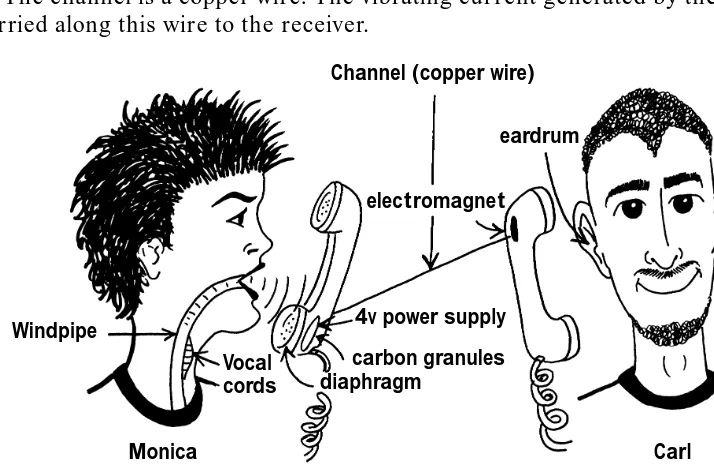
we’ll call Carl and Monica, using the telephone. What follows is a wordy description of how the telephone works. Refer to Figure 1.4 to help you with the terms.
The transmitter consists of Monica (who is talking) and the transmitting (bottom) end of the telephone. Monica speaks, and her vocal cords vibrate. This causes vibra-tions in the air, which travel through and out her mouth, and then travel to the bottom end of the telephone. Inside the bottom end of the telephone is a diaphragm. When the vibrations of the air arrive at this diaphragm, it, like an eardrum, begins to vibrate. Directly behind the diaphragm are a bunch of carbon granules. These gran-ules are part of an electrical circuit, which consists of a 4-V source, copper wire, and the carbon granules. The carbon granules act as a resistor (with variable resistance) in the circuit. When the diaphragm is pushed back by the vibrating air, it causes the carbon granules (right behind it) to mush together. In this case, the granules
act like a low-resistance resistor in the circuit. Hence, the current flowing though the electric circuit is high (using the well-known
V
=
R
⋅
I
rule). When the diaphragm is popped out by the vibrating air, it causes the carbon granules (right behind it) to separate out. In this case, those carbon granules are acting like a high-resistance resistor in the electrical circuit. Hence, the current flowing though the circuit is low. Overall, vibrations in the diaphragm (its “pushing back” and “popping out”) cause the same vibrations (frequencies) to appear in the current of the electrical circuit (via those carbon granules). [image:26.531.51.408.367.604.2]The channel is a copper wire. The vibrating current generated by the transmitter is carried along this wire to the receiver.
Figure 1.4
Monica and Carl talking on a telephone
Channel (copper wire)
Windpipe
Vocal cords
TRANSMITTER RECEIVER
electromagnet eardrum
4v power supply
carbon granules diaphragm
The receiver consists of two parts: the receiving (top) part of the telephone, and Carl’s ear. The current, sent along the copper wire, arrives at the top end of the tele-phone. Inside this top end is a device called an electromagnet and right next to that is a diaphragm. The current, containing all of Monica’s talking frequencies, enters into the electromagnet. This electromagnet causes the diaphragm to vibrate with all of Monica’s talking frequencies. The vibrating diaphragm causes vibrations in the air, and these vibrations travel to Carl’s ear. His eardrum vibrates, and these vibrations cause electrical signals to be sent to his brain, which interprets this as Monica’s sound.
1.3 Analog and Digital Communication Systems
The last part of this chapter is dedicated to explaining what is meant by analog and digital communication systems, and then explaining why digital communication systems are the way of the future.
1.3.1 Some Introductory Definitions
An analog signal is a signal that can take on any amplitude and is well-defined at every time. Figure 1.5(a) shows an example of this. A discrete-time signal is a signal that can take on any amplitude but is defined only at a set of discrete times. Figure 1.5(b) shows an example. Finally, a digital signal is a signal whose amplitude can take on only a finite set of values, normally two, and is defined only at a discrete set of times. To help clarify, an example is shown in Figure 1.5(c).
Figure 1.5 (a) An analog signal; (b) a discrete time signal; and (c) a digital signal
x(t) x(t)
t t
(a) (b)
T 2T 3T 4T ...
x(t)
t
(c) T
0 1
1.3.2 Definitions
An analog communication system is a communication system where the information signal sent from point A to point B can only be described as an analog signal. An example of this is Monica speaking to Carl over the telephone, as described in Section 1.2.2.
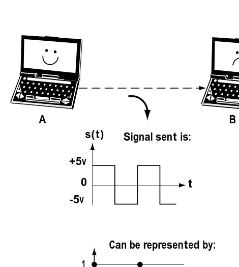
[image:28.531.112.347.292.554.2]A digital communication system is a communication system where the information signal sent from A to B can be fully described as a digital signal. For example, con-sider Figure 1.6. Here, data is sent from one computer to another over a wire. The computer at point A is sending 0s or 1s to the computer at point B; a 0 is being repre-sented by –5 V for a duration of time T and a 1 is being reprerepre-sented by a +5 V for the same duration T. As I show in that figure, that sent signal can be fully described using a digital signal.
Figure 1.6 A computer sending information to another computer
0 +5v
-5v
0 1
s(t)
t t
B A
Signal sent is:
Can be represented by:
1.3.3 And Digital Became the Favorite
Digital communication systems are becoming, and in many ways have already be-come, the communication system of choice among us telecommunication folks. Certainly, one of the reasons for this is the rapid availability and low cost of digital components. But this reason is far from the full story. To explain the full benefits of a digital communication system, we’ll use Figures 1.7 and 1.8 to help.
Let’s first consider an analog communication system, using Figure 1.7. Let’s pretend the transmitter sends out the analog signal of Figure 1.7(a) from point A to point B. This signal travels across the channel, which adds some noise (an unwanted signal). The signal that arrives at the receiver now looks like Figure 1.7(b). Let’s now consider a digital communication system with the help of Figure 1.8. Let’s imagine that the transmitter sends out the signal of Figure 1.8(a). This signal travels across the channel, which adds a noise. The signal that arrives at the receiver is found in Figure 1.8 (b).
Figure 1.7 (a) Transmitted analog signal; (b) Received analog signal
Figure 1.8 (a) Transmitted digital signal; (b) Received digital signal
0 +5v
-5v s(t)
t 0 +5v
-5v s(t)
t 1 0 1
(a) (b)
Noise
s(t) r(t)
t t
(a) (b)
Here’s the key idea. In the digital communication system, even after noise is added, a 1 (sent as +5 V) still looks like a 1 (+5 V), and a 0 (–5 V) still looks like a 0 (–5 V). So, the receiver can determine that the information transmitted was a 1 0 1. Since it can decide this, it’s as if the channel added no noise. In the analog communication system, the receiver is stuck with the noisy signal and there is no way it can recover exactly what was sent. (If you can think of a way, please do let me know.) So, in a digital communication system, the effects of channel noise can be much, much less than in an analog communication system.
1.3.4 Making It Digital
A number of naturally occurring signals, such as Monica’s speech signal, are analog signals. We want to send these signals from one point, A, to another point, B. Because digital communication systems are so much better than analog ones, we want to use a digital system. To do this, the analog signal must be turned into a digital signal. The devices which turn analog signals into digital ones are called source coders, and we’ll spend all of Chapter 4 exploring them. In this section, we’ll just take a brief peek at a simple source coder, one that will turn Monica’s speech signal (and anyone else’s for that matter) into a digital signal. The source coder is shown in Figure 1.9.
It all begins when Monica talks into the telephone, and her vibrations are turned into an electrical signal by the bottom end of the telephone talked about earlier. This electrical signal is the input signal in Figure 1.9. We will assume, as the telephone company does, that all of Monica’s speech lies in the frequency range of 100 Hz to 4000 Hz.
The electrical version of Monica’s speech signal enters a device called a sampler. The sampler is, in essence, a switch which closes for a brief period of time and then opens, closing and opening many times a second. When the switch is closed, the electrical speech signal passes through; when the switch is open, nothing gets
through. Hence, the output of the sampler consists of samples (pieces) of the electrical input.
Figure 1.9 A simple source coder
Quantizer Symbol-to-bit Mapper Sampler
As some of you may know (and if you don’t, we’ll review it in Chapter 4, so have no worries), we want the switch to open and close at a rate of at least two times the maximum frequency of the input signal. In the case at hand, this means that we want the switch to open and close 2 × 4000 = 8000 times a second; in fancy words, we want a sampling rate of 8000 Hz.
After the switch, the signal goes through a device called a quantizer. The quan-tizer does a simple thing. It makes the amplitude of each sample go to one of 256 possible levels. For example, the quantizer may be rounding each sample of the incoming signal to the nearest value in the set {0, 0.01, 0.02, ..., 2.54, 2.55}.
Now, here’s something interesting. There is a loss of information at the quantizer. For example, in rounding a sample of amplitude 2.123 to the amplitude 2.12, informa-tion is lost. That informainforma-tion is gone forever. Why would we put in a device that intentionally lost information? Easy. Because that’s the only way we know to turn an analog signal into a digital one (and hence gain the benefits of a digital communication system). The good news here is engineers (like you and me) build the quantizer, and we can build it in a way that minimizes the loss introduced by the quantizer. (We’ll talk at length about that in Chapter 4.)
After the quantizer, the signal enters into a symbol-to-bit mapper. This device maps each sample, whose amplitude takes on one of 256 levels, into a sequence of 8 bits. For example, 0.0 may be represented by 00000000, and 2.55 by 11111111. We’ve now created a digital signal from our starting analog signal.
1.4 Congrats and Conclusion
Problems
1. Briefly describe the following: (a) telecommunication system (b) communication system
(c) the difference between a communication system and a telecommunication system.
(d) digital communications (e) analog communications
(f) the main reason why digital communications is preferred (to analog communications).
2. Describe the function of the following: (a) source coder
(b) quantizer (c) sampler
1
2 3
4
5 6
Copper wire
2
Telecommunication
Networks
F
irst, and always first, a definition. A telecommunication network is a telecommuni-cation system that allows many users to share information.2.1 Telecommunication Network Basics
2.1.1 Connecting People with Telephones
Let’s say I have six people with telephones. I want to connect them together so they can speak to one another. One easy way to connect everyone is to put copper wires everywhere. By that, I mean use a copper wire to connect person 1 to person 2, a wire to connect person 1 to person 3, ..., a wire to connect person 1 to person 6, ..., and a wire to connect person 5 to person 6. I’ve shown this solution in Figure 2.1. But, ugh, all these wires! In general, I need N(N–1)/2 wires, where N is the number of people. So with only six people I need 15 wires, with 100
people I need 49,950 wires, and with a million people I need 499,999,500,000 wires. Too many wires.
Let’s consider another way to connect users: put a switching center between the people, as shown in Figure 2.2. The early switchboards worked like this: Gretchen picks up her phone to call Carl. A connection is immediately made to Mavis, a sweet elderly operator seated at the switching center. Mavis asks Gretchen who she wants to talk to, and Gretchen says “Carl.” Mavis then physically moves wires at the switch-ing center in such a way that the wire from Gretchen’s phone is directly connected to Carl’s wire, and Gretchen and Carl are now ready to begin
their conversation. Figure 2.1
Figure 2.2
Phones connected by a switching center
1
2 3
4
5 6
Switching Center
The manual switching center, oper-ated by people like Mavis, was the only way to go until a little after 1889 when Almon B. Strowger, a mortician by trade, invented the first automatic switching center. It seems that Almon suddenly found that he was no longer getting any business. Sur-prised, he investigated and discovered that the new telephone operator was also married to the competition ... and she was switching all funeral home calls to her husband. Determined to keep his mortician business alive (no pun intended), Almon created the first automatic switching center. These switching centers do not require anyone (and hence no competitor’s wife) to transfer calls. Entering a 7-digit phone number automatically sets up the connection at the switching center. Today, all switching centers are automatic.
Just briefly, how many wires are needed by a network using a switching center? Only N, where N is the number of users. That’s far fewer than the many-wire system introduced first.
2.1.2 Connecting More People, Farther Apart
Let’s take this switching center idea a bit further. Consider Figure 2.3. A bunch of people are connected together in Fort Collins, Colorado, by a switching center in downtown Fort Collins. Then, in nearby Boulder, another group of people are con-nected together by a second switching center. How does someone in Boulder talk to a friend in Fort Collins? One easy way is to simply connect the switching centers, as shown in Figure 2.3. If we put several wires between the Fort Collins and Boulder switching centers, then several people in Fort Collins can talk to people in Boulder at the same time.
1 1
2 3 2 3
4 4
5 5
6 6
Switching Center Switching Center
Fort Collins, CO Boulder, CO
Figure 2.3 Connections between
Consider now a number of other nearby cities, say Longmont and Denver. The folks in these towns want to talk to their friends in Boulder and Fort Collins. We could connect all the switching centers together, as shown in Figure 2.4. Alternatively, we could have a “super” switching center, which would be a switching center for the switching centers, as shown in Figure 2.5.
Switching Center Switching
Center
Switching Center
Switching Center
Longmont Denver
1 1
1 1
2 2
2 2
3 3
3 3
4 4
4 4
5 5
5 5
6 6
6 6
Boulder Fort Collins
Switching Center Switching
Center
Switching Center
Switching Center
Longmont Denver
1 1
1 1
2 2
2 2
3 3
3 3
4 4
4 4
5 5
5 5
6 6
6 6
Boulder Fort Collins
"Super"
Switching
[image:36.531.44.420.136.340.2]Center
Figure 2.4 Connecting all the switching centers together
2.1.3 Multiplexing—An Alternative to a Lot of Wire
Let’s go back to the Fort Collins and Boulder people in Figure 2.3. Let’s say we’ve connected their switching centers so they can talk to each other. As more people in Fort Collins want to talk to more people in Boulder, more and more wires need to be added between their switching centers. It could get to the point where there are far too many wires running between the switching centers. The skies around Fort Collins could grow dark under the cover of all these wires. This probably wouldn’t be true of a smaller town like Fort Collins, but it was true of big cities like New York.
Finally, someone said, “Something must be done!’’ and multiplexing was invented. Multiplexing refers to any scheme that allows many people’s calls to share a single wire. (We’ll talk more about this in Chapter 11, but a brief introduction now is useful.)
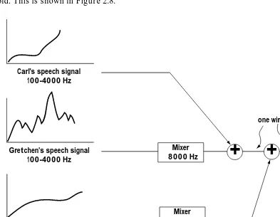
First There Was FDM
FDM, short for frequency division multiplexing, was the first scheme created to allow people’s calls to share a wire. Let’s say Carl, Gretchen, and Monica all want to make a call from Fort Collins to Boulder. We only want to use one wire to connect calls be-tween the two towns. This is shown in Figure 2.6. Carl’s speech, turned into a current on a wire, contains the frequencies 100 to 4000 Hz. His speech is left as is. Gretchen’s speech, turned into an electrical signal on a wire, also contains the frequencies 100 to 4000 Hz. A simple device called a mixer (operating at 8000 Hz) is applied to her speech signal. This device moves the frequency content of her speech signal, and the frequen-cies found at 100 Hz to 4,000 Hz are moved to the frequenfrequen-cies 8,100 Hz to 12,000 Hz, as shown in Figure 2.7.
Switching Center
Switching Center
Boulder Fort Collins
Carl, Gretchen and Monica's voices
[image:37.531.42.388.395.597.2]all on one wire
Figure 2.6
Because Carl and Gretchen’s calls are now made up of different frequency com-ponents, they can be sent on a single wire without interfering with one another. This too is shown in Figure 2.7. We now want to add Monica’s speech signal, since she too is making a call from Fort Collins to Boulder. A mixer, this one operating at 16,000 Hz, is applied to her speech signal. This moves the frequency content of Monica’s speech to 16,100 Hz to 20,000 Hz, as shown in Figure 2.7. Because Monica’s speech signal is now at different frequencies than Carl and Gretchen’s speech signals, her signal can be added onto the same wire as Carl and Gretchen’s, without interfering. (Again, take a peek at Figure 2.7.)
Over in Boulder, we’ve got a wire with Carl, Gretchen, and Monica’s speech on it, and we need to separate this into three signals. First, to get Carl’s signal, we use a device called a low-pass filter (LPF). The filter we use only allows the frequencies in 0 to 4000 Hz to pass through; all other frequency components are removed. So, in our example, this filter passes Carl’s speech, but stops Gretchen’s and Monica’s speech cold. This is shown in Figure 2.8.
Carl's speech signal 100-4000 Hz
Gretchen's speech signal 100-4000 Hz
Monica's speech signal 100-4000 Hz
one wire Mixer
8000 Hz
Mixer 16,000 Hz
[image:38.531.36.429.271.576.2]+
+
Figure 2.7
Next, we want to recover Gretchen’s speech signal. This is a two-part job. First, a bandpass filter (BPF) is applied, with start frequency 8,000 Hz and stop frequency 12,000 Hz. This filter allows only the frequencies between 8,000 Hz and 12,000 Hz to pass through, cutting out every other frequency. In the case at hand, this means that only Gretchen’s speech signal gets through the filter. This is shown in Figure 2.8. We still have one task left. Gretchen’s speech signal has been moved from 100–4,000 Hz to 8,100–12,000 Hz. We want to bring it back to the original 100–4000 Hz. This is done by applying a mixer (operating at 8,000 Hz), which returns Gretchen’s voice signal to its original frequency components.
Monica’s signal is recovered on a single wire in much the same way as Gretchen’s, and, rather than use many words, I’ll simply refer you to Figure 2.8.
Carl, Gretchen and Monica's speech
on one wire
LPF 0-4000 Hz
BPF 8000-12000 Hz
BPF 16000-20000 Hz
Mixer 8000 Hz
Mixer 16000 Hz
Carl's speech signal
Gretchen's speech signal
Monica's speech signal
Figure 2.8 Getting three speech signals back from one wire in FDM
Along Came TDM
TDM, short for time-division multiplexing, is the second commonly used technique to let several people’s speech share a single wire. TDM works like this. Let’s say we’ve again got Carl, Gretchen, and Monica, who all want to make their calls from Fort Collins to Boulder. Carl, Gretchen, and Monica’s speech sounds are first turned into an electrical signal on a wire by their phones, as explained in Chapter 1. Then, their electrical speech signals are turned into digital signals, again as explained in Chapter 1. The digitized, electricized versions of the speech signal are the incoming signals that will share a wire. Figure 2.9 shows these incoming signals.
Gretchen at home
Carl at the office
Class 5 Switching Center
[image:40.531.37.424.52.265.2](end office)
Figure 2.10 Connecting a local call: the local loop
2.2 POTS: Plain Old Telephone System
Enough of the basics. Let me now introduce you to a telecommunication network currently in use. In fact, it’s the most frequently used telecommunication network in the world. It’s called POTS, short for Plain Old Telephone System. We’ll be consider-ing the phone connections exclusively in Canada and the United States, but keep in mind that similar systems exist worldwide.
2.2.1 Local Calls
Let’s say Gretchen, at home in Fort Collins, decides to call Carl, who is hard at work at CSU writing this book. Here’s
how the call gets from Gretchen to Carl. First,
Gretchen’s phone turns her sounds into an analog electrical signal, as explained in Section 1.2.2.
This analog electrical signal is sent along a copper wire (called a twisted-pair cable) to the switching center called the Class 5 switching center, or end office (Figure 2.10).
t
t t T
T T Carl's digital speech
Gretchen's digital speech
Monica's digital speech
...
...
...
... "The Big Switch"
Carl, Gretchen & Monica's digital speech
t
Carl
Gretchen
Monica
T/3
T
The switching center knows Gretchen’s call is a local call to Carl’s office (based on a 7-digit number she initially dialed), and it sends Gretchen’s speech signal down the copper wire that connects to Carl’s office. This signal then enters Carl’s phone, which turns the electrical signal back into Gretchen’s speech sounds, and there we have it. This part of the phone system is called the local loop. There are about 20,000 end offices in Canada and the United States.
2.2.2 Long Distance Calls
Connecting the Call
Let’s say that Carl’s mom, Mona, who lives in the cold of Montreal, Canada, wants to call Carl in Colorado and see if he’s eating well (yes, Mom, I’m eating well). How would the telephone system connect this call? We’ll use Figure 2.11 as our guide. First, Mona’s Are you eating well? sounds are turned into an analog electrical signal by her telephone. This electrical signal is sent along copper wire to the end office (or class 5 switching center). The end office, realizing that this isn’t a local call, does two things: (1) it mixes Mona’s signal with other people’s voice signals (that are also not local calls), using multiplexing; then, (2) it takes the mix of Mona’s speech signal and the other people’s speech signals and sends this mix to a bigger switching center, called a Class 4 switching center, or toll center, shown in Figure 2.11. The toll center is con-nected to three sets of things.
[image:41.531.40.398.351.609.2]Class 5 End Office Class 4 Toll Center Class 4 Toll Center Class 4 Toll Center Class 4 Toll Center Class 4 Toll Center Class 4 Toll Center Class 3 Primary Center Class 3 Primary Center Class 3 Primary Center Class 3 Primary Center Class 2 Class 2 Class 2 Class 2 Class 1 Class 1 Class 5 End Office Class 5 End Office Class 5 End Office Class 5 End Office Class 5 End Office A B C D E F AA BB Multiplexing of Mona's speech and other speech
Figure 2.11 A long-distance call in
First, it’s connected to a number of end offices (A, B, C, and D in Figure 2.11), each end office like the one that Mona’s call came from. If Mona’s call was intended for a phone that was connected to end office C for example, then Mona’s speech would be sent to end office C and from there to the intended phone.
The second thing the Class 4 switching center (toll center) is connected to is other Class 4 switching centers (BB in Figure 2.11). If the call is intended for a phone connected to end office E, then it would likely be sent to toll center BB, then to end office E, and then to the intended telephone.
The third thing a Class 4 switching center is connected to is an even bigger switching center, which is called (no big surprise) a Class 3 switching center (also called a primary center). If Mona’s call is going to a phone not connected to any of the end offices available from toll centers AA or BB, then Mona’s speech moves along to the class 3 switching center.
The good news is that the Class 3 switching center works in pretty much the same way as the Class 4 switching center. Basically, from the Class 3 switching center, Mona’s call can go to: (1) any Class 3, 4, or 5 switching center that is connected to the Class 3 switching center holding Mona’s speech—it will go that route if the intended phone is connected to one of these Class 3, 4, or 5 switching centers; otherwise, (2) the call will be switched to an even bigger switching center, called the Class 2 switching center (and also called the sectional center).
Let’s say Mona’s call heads out to the Class 2 switching center. From here it gets to Carl in one of two ways: (1) if Carl’s phone is connected to a Class 2, 3, 4, or 5 switching center that is directly connected to the Class 2 switching center containing Mona’s voice, then Mona’s voice gets sent to that switching center; otherwise, (2) Mona’s call will go to the last, biggest switching center, the Class 1 switching center (or regional center). The Class 1 switching center will then send the call to either a Class 1, 2, 3, 4, or 5 switching center that it’s connected to, depending on which center is most directly connected to Carl’s phone.
And that, my friends, is how Mona’s concern about Carl’s eating habits gets from Mona in Montreal to Carl in Colorado. It’s a 5-level hierarchy of switching centers. There are some 13,000 toll centers, 265 primary centers, 75 sectional centers, and 12 regional centers.
2.2.3 The Signals Sent from Switching Center to Switching Center
A telephone call starts out with the phone in your hand. That call goes to a Class 5 switching center. If the call is local, it goes from that Class 5 switching center right to the person you’re talking to. If the call is not local, the Class 5 switching center puts the call together with other long-distance calls, and sends them together to a Class 4 switching center. Let’s look at the signal created at a Class 5 switching center that is sent to a Class 4 switching center.
Class 5 to Class 4
The Class 5 switching center gets the call you place. It also gets a lot of other calls from your neighborhood. When the Class 5 switching center realizes there are a bunch of calls that are not in its area (and instead are long-distance calls), it puts these signals together and sends them out. Specifically, it puts the signals together as shown in Figure 2.12:
A A
t
Your call
8000 samples/sec
T=1/8000=0.125ms #1
#2
#3
#24 . . .
. . .
Symbol to bit mapper Quantizer 1
Add bit The
Big Switch
Class 5 Switching Center
Forces each amplitude to the nearest one out of 256 permitted
output amplitudes
To class 4
*
*
. . .
A
t T = 0.125ms Piece from
line #1
Piece from line #2
Piece from line #24
[image:43.531.16.416.248.552.2]T/24
1. First, at the line marked #1, is your call. But that is only one thing coming into the Class 5 switching center. The center takes your call and at the same time takes 23 others, for a total of 24 calls. Those calls incoming to the Class 5 switch-ing center are the lines marked #1 to #24.
2. The switching center puts these 24 calls on a single line using TDM. That idea is explained in Section 2.1.3, but here are some more details explaining exactly what the Class 5 switching center does.
2a. Each voice call is sampled. Specifically, samples of each voice call are taken at a rate of 8000 samples/second (i.e., at 8000 Hz). That means that each sample taken from a voice call lasts a total time of T = 1/8000 = 0.125 ms.
2b. Each sampled voice signal meets “the big switch.” The big switch makes contact with each digital voice signal briefly once every 0.125 ms. As a result, the signal that ends up on the wire following “the big switch” is a collection of all 24 voice signals. This is shown in Figure 2.12 better than my words can explain.
2c. On the wire following the big switch, we have all 24 voice samples
smooshed together in the time T = 0.125 ms. The number of samples in each second is now 24 × 8,000 samples/second = 192,000 samples/second.
3. The 192,000 samples/second on our wire now enter through a device called a quantizer. The quantizer simply changes the amplitude of the incoming samples. Each incoming sample, which has some amplitude A, is mapped to an outgoing sample whose amplitude is one of 256 possible values.
4. Each sample, with an amplitude that is now one of 256 levels, can be fully represented by a set of 8 bits. (This is because with 8 bits we can represent all integers between 1 and 256.) A device called a symbol-to-bit mapper takes each sample with one of 256 possible amplitudes, and represents it with 8 bits. While before we had 24 samples in each 0.125 ms, we now have 24 × 8 = 192 bits in each 0.125 ms.
5. To tell people where each set of 192 bits begins and ends, an extra bit (a 0) is squeezed in so that we now have 193 bits in each 0.125 ms. That means we have a bit rate of 193 bits/0.125 ms = 1.544 Mb/s.
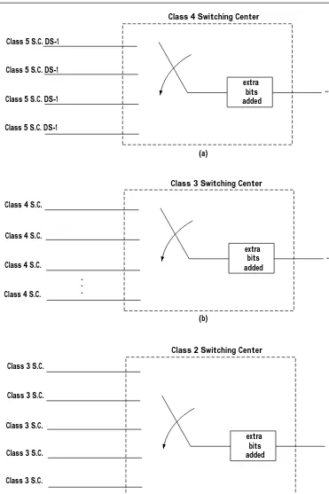
Other Signals between Switching Centers
Figure 2.13 shows the different signals sent between different switching centers. Coming into a Class 4 center is a DS-1 signal. It is likely that this incoming signal will need to be sent to the Class 3 center. If that’s the case, the Class 4 center creates a very special signal for transmission up to Class 3. Specifically, it takes four DS-1 signals that are coming into it (from Class 5 centers) and puts these signals together onto a single wire using TDM. It adds a few extra bits to help the Class 3 center identify the beginning of what it gets and the end of it. When it’s all said and done, the signal that moves from Class 4 to Class 3 is a stream of bits with a bit rate of 6.312 Mb/s. That signal is called a DS-2 signal.
A signal enters into a Class 3 switching center. This signal might need to move up to a Class 2 switching center. In that case, the Class 3 switching center puts together a special signal just for Class 2. It takes seven DS-2 signals that are coming into it (from Class 4 centers), and puts them together on a single wire using TDM. It adds a few extra bits to help the Class 2 office identify places where bit streams begin and end. Ultimately, it sends a signal to Class 2 that is a stream of bits with a bit rate of 44.736 Mb/s. This signal is called a DS-3 signal.
Finally, it is possible in POTS that a signal arriving at a Class 2 switching center might be sent up to a Class 1 switching center. If that’s the case, Class 2 puts together a special signal for Class 1. Specifically, a Class 2 center takes five of the DS-3 signals that come into it (from Class 3 centers), and packages them together on a single wire using TDM. Including a few extra bits to make the package look nice for Class 1, the stream of bits sent to Class 1 has a bit rate of 274.1746 Mb/s. This signal is called DS-4.
What I’ve said so far is true, but not the complete truth. In general, it is possible in POTS that DS-1, DS-2, DS-3, and DS-4 signals could be found between any two switching centers. For example, I presented DS-3 as the signal Class 3 sends to Class 2 switching centers. It is also possible in POTS that Class 3 sends a DS-2 signal to Class 2.
2.3 Communication Channels
So far in our discussion, communication signals have been sent on wires. However, there are a number of different ways in which a communication signal can be sent from one point to another. Using a wire is just one way—POTS likes and embraces this way. In this section, I’ll outline the different ways you can send a signal from one point to another—that is, I’ll outline different communication channels.
2.3.1 Transmission Lines (Wires)
extra bits added
extra bits added
extra bits added
...to class 3 DS-2
...to class 2 DS-3
...to class 1 DS-4 Class 5 S.C. DS-1
Class 4 S.C.
Class 3 S.C. Class 3 S.C. Class 5 S.C. DS-1
Class 4 S.C.
Class 3 S.C. Class 5 S.C. DS-1
Class 4 S.C.
Class 3 S.C. Class 5 S.C. DS-1
Class 4 S.C.
Class 3 S.C.
Class 4 Switching Center
Class 3 Switching Center
Class 2 Switching Center
(c) (b) (a)
[image:46.531.45.416.46.603.2]. . .
Figure 2.13
In twisted-pair cable, a signal is sent from one point to another as a current along a wire. Signals that are sent in the frequency range of 0 to 1 MHz can be supported. The most common use for twisted-pair cables is in POTS. It forms most of the local loop connections. Specifically, in POTS, an insulated twisted-pair cable leaves from a home and is combined with many other twisted-pair cables from neighboring homes. You end up with one, big fat set of twisted-pair cables sent to the end office (Class 5).
Coaxial cables are the second type of “wire” used to send communication signals. In coaxial cables, the communication information is sent as a current along a wire. Coaxial cables can support signals in the 100 kHz to 400 MHz range (a much larger range of frequencies than the twisted-pair cable can support). Perhaps the most common use of coaxial cable is in connections from TV cable providers to your home. Other uses include long-distance lines in POTS and local area networks (LANs), discussed a little later in this chapter.
2.3.2 Terrestrial Microwave
Another way in which information can be sent from one point to another is by use of (1) a modulator, which turns the incoming information signal into a high-frequency electrical signal on a wire; and (2) an antenna, which turns the high-frequency signal into an electromagnetic wave sent through the atmosphere. At the receiver side, you use (1) a receiver antenna, which picks up the incoming electromagnetic wave and turns it back into the high-frequency electrical signal, and (2) a demodulator, which returns the high-frequency electrical signal back to the original information signals. Some examples of communication systems which send information in this way are radio stations, wireless communication systems (later in this chapter), and terrestrial microwave, which I’ll explain right now so you can get a better understanding of this idea.
A terrestrial microwave transmitter is shown in Figure 2.14. I’ll explain its work-ings here in three points.
1. In Figure 2.14 you see the incoming information signal. In this example, the incoming information signal contains voice signals; specifically, it contains two DS-3 signals combined on a single wire using TDM methods.
2. The incoming information signal enters a modulator, and the modulator maps the incoming signal into a high-frequency electrical signal. For example, the modulator may map the incoming signal so that it is now centered around 3 GHz, 11 GHz, or 23 GHz.
Between the transmitter and receiver we place some devices called repeaters, shown in Figure 2.15. Repeaters are placed every 26 miles (40 kilometers). The re-peater may do one of two things: (1) it may simply amplify and retransmit the signal at a higher power (non-regenerative repeater); or (2) it may receive the incoming signal, remove noise as best it can through a demodulation/remodulation process, and then retransmit the signal at a high power (regenerative repeater). We use repeaters for two reasons. First, because of the curvature of the earth, the transmit antenna will be hidden from the receiver if we do not place a repeater between the transmitter and receiver (Figure 2.15). Second, repeaters can be useful in reducing the impact of channel noise.
...
Modula tor
Parabolic dish antenna
High frequency signal (centered around 3 GHz, for example)
EM wave
2 DS-3 signals
26 mi.
26 mi.
26 mi.
Transmitter
Repeater #1
Repeater #2
[image:48.531.43.419.194.559.2]Receiver Figure 2.14 Terrestrial microwave
system transmitter
Receiver antenna
EM wave
High frequency electrical signal
Demodulator
Information-bearing signal
Figure 2.16 Terrestrial microwave receiver
Finally, after travelling through the repeaters, the signal arrives at the receiver, shown in Figure 2.16. First, a receiver antenna is applied to return the signal to an electrical signal of a frequency of 3 GHz. Then, a demodulator is applied that returns the high-frequency signal to the original information signal.
The terrestrial microwave system just described typically operates in frequency ranges of 1 GHz to 50 GHz, and it has been applied in a number of different communication systems. For
example, it has been used as a part of POTS, to connect two Class 2 switching centers separated by terrain such as swamp where it is very difficult to lay wire. This terrestrial
microwave system has also been set up to connect large branches of big companies. It has also been implemented as a backup to fiber-optic links (later in this chapter).
2.3.3 Satellite Connections
With satellite connections, a communication system is set up as shown in Figure 2.17. Here, a transmitter takes the incoming information signal, uses a modulator to turn it into a high-frequency signal, and then uses an antenna to turn the signal into an elec-tromagnetic wave sent through the atmosphere (just as in terrestrial microwave).
Solar panels generating electricity to operate satellite Satellite
Modula
tor Demodula
tor
Information signal
Information signal
High-frequency electrical signal
High-frequency electrical signal Ocean
6 GHz 4 GHz
Figure 2.17 Satellite communication
This signal is then sent up to a satellite in orbit around the earth. Specifically, the satellite is placed at 36,000 km (22,300 miles), and at that altitude it orbits the Earth at 6,870 mph. Moving at this speed, the satellite appears to be stationary when looked at from the equator, and so it is said to be in a geo-stationary orbit. The satellite picks up the signal and does two things:
(1) it acts as a repeater; and
(2) it shifts the frequency (for example, from 6 GHz to 4 GHz) and sends it back down to earth in the direction of the receiver. Modern satellites are being built which can do more signal processing at the satellite itself, but we won’t go into those details here.
The signal leaves the satellite and heads back to the receiver on Earth. At that receiver, an antenna is applied that turns the incoming electromagnetic wave back to an electrical signal, and that electrical signal is returned to the original information signal by a device called a demodulator.
Satellite communications operate in a number of frequency bands. Here are some of them: (1) C-band, which refers to 6-GHz uplink (“up” to the satellite) and 4-GHz downlink (“down” to the receiver); (2) Ku-band, which is 14-GHz uplink/12-GHz downlink; and (3) ACTS which refers to 30-GHz uplink/20-GHz downlink.
Some of the many uses of satellite communications include satellite TV distribu-tion, live TV transoceanic links, telephone communications over the oceans, backup to fiber-optic links, and GPS (Global Positioning System). GPS refers to a system of satellites which enables anyone, using a hand-held device, to determine their exact position on our planet (very useful for ships, backpackers, and companies with large fleets of trucks/cars/aircraft).
2.3.4 Fiber-optic Links
Fiber-optic cable is a revolution in connecting transmitters to receivers. It seems possible to support incredible—and I do mean incredible—rates of information along this cable. Using fiber-optic cable, it appears that we can support 1014 bits/s, at the
very least. Right now, we don’t know how to send information at this high a rate (although we’re moving in that direction)—we also don’t have that much information to send yet!
The fiber-optic cable, which you can also see in Figure 2.18, is made up of two parts: a core and a cladding. The light travels down the core. It remains in the core and never leaves it (never entering the cladding). This is because the two materials chosen for core and cladding are carefully selected to ensure that total internal refrac-tion occurs—that means that as light enters the boundary between core and cladding, it is bent in such a way that it remains in the core. (For more on this, check out a physics book.)
At the receiver side, the light signal, which has made it through the fiber-optic cable, must be returned to an electrical signal. That job is done using a detector, as seen in Figure 2.17. The detector might be, for example, a PIN diode or an APD (avalanche photo diode).
The light sent down the fiber-optic cable corresponds to an electromagnetic wave with a frequency in the range of 1014 to 1015 Hz. As mentioned already, the system
appears capable of sending information at rates of 1014 bits/s.
Because of the incredible promise of fiber-optic cable, these cables are being placed everywhere. They have even been placed on the ocean floor between North America and Europe, competing with and in many cases replacing satellite links. Fiber-optic links are being used to connect switching centers in POTS. They are limiting the use of coaxial cable and twisted-pair cable to areas where they have already been put in place.
Emitter Detector Incoming information
on electrical signal
Outgoing information on a light wave
Original information on electrical signal Cladding
Core
Light signal