ACLAS – a method to define geologically significant lineaments from potential fields data

ACLAS

—

A method to define geologically significant lineaments

from potential-field data

Lorenzo Cascone

, Chris Green

, Simon Campbell

, Ahmed Salem

, and Derek Fairhead

ABSTRACT

Geologic features, such as faults, dikes, and contacts appear as lineaments in gravity and magnetic data. The automated co-herent lineament analysis and selection (ACLAS) method is a new approach to automatically compare and combine sets of lineaments or edges derived from two or more existing enhance-ment techniques applied to the same gravity or magnetic data set. ACLAS can be applied to the results of any edge-detection algorithms and overcomes discrepancies between techniques to generate a coherent set of detected lineaments, which can be more reliably incorporated into geologic interpretation. We have determined that the method increases spatial accuracy, removes artifacts not related to real edges, increases stability, and is quick to implement and execute. The direction of lower density or

susceptibility can also be automatically determined, represent-ing, for example, the downthrown side of a fault. We have evalu-ated ACLAS on magnetic anomalies calculevalu-ated from a simple slab model and from a synthetic continental margin model with noise added to the result. The approach helps us to identify and discount artifacts of the different techniques, although the suc-cess of the combination is limited by the appropriateness of the individual techniques and their inherent assumptions. ACLAS has been applied separately to gravity and magnetic data from the Australian North West Shelf; displaying results from the two data sets together helps in the appreciation of similarities and differences between gravity and magnetic results and indicates the application of the new approach to large-scale structural mapping. Future developments could include refinement of depth estimates for ACLAS lineaments.

INTRODUCTION

The value of gravity and magnetic data to map geologic structures has been long recognized. Over the years, many derivatives and trans-formations of data grids have been developed to help highlight and refine geologic boundaries and lineaments; only a selection are mentioned below. These techniques are often tested on simple geo-metric models, but they have nonetheless been found to assist and speed the map-based interpretation of gravity and magnetic data.

The total horizontal derivative (THD) of pseudogravity was used byCordell and Grauch (1985)to map lineaments from magnetics in a semiautomated manner. The method was also applied to derivatives of gravity data byBlakely and Simpson (1986), who develop an au-tomated approach to picking maxima from derivative grids. The ana-lytic signal or total gradient (Nabighian, 1972;Roest et al., 1992) has

been used to define lineaments at all latitudes. Transformations de-rived from the analytic signal have also been introduced: local wave-number (Thurston and Smith, 1997) and tilt (Miller and Singh, 1994; Verduzco et al., 2004). A range of other techniques using a combi-nation of derivatives has been developed, such as the theta map (Wijns et al., 2005) and TDX (Cooper and Cowan, 2006). Other techniques include magnitude transforms of magnetic data (Stavrev and Gerov-ska, 2000), the multiscale method (Fedi, 2002), curvature-based meth-ods (Hansen and deRidder, 2006; Phillips et al., 2007), and the monogenic signal transformation (Hidalgo-Gato and Barbosa, 2015). All of these methods estimate the locations of lineaments, often edges of geologic bodies or faults, and some can also be used to estimate the depth to the source of the magnetic anomaly. Various authors (Phillips, 2000; Pilkington and Keating, 2004, 2010;

Manuscript received by the Editor 27 June 2016; revised manuscript received 3 February 2017; published ahead of production 1 May 2017; published online 13 June 2017.

1_{Formerly GETECH Group plc, Leeds, UK; presently Repsol Exploration SA, Geophysics Team, Madrid, Spain. E-mail: [email protected].} 2_{GETECH Group plc, Leeds, UK and University of Leeds, Leeds, UK. E-mail: [email protected]; [email protected]; jamesderekfairhead@}

gmail.com.

3_{GETECH Group plc, Leeds, UK. E-mail: [email protected].}

© 2017 Society of Exploration Geophysicists. All rights reserved.

G87

Pilkington, 2007) have analyzed the advantages and disadvantages of the available methods. They find that lineaments from different derivatives and transforms are sensitive in different ways to the short-wavelength noise, line noise, or complexity of the source distribution.

A particular concern with these techniques is highlighted by Pil-kington (2007), who calculates the edge location that would be pre-dicted by various edge-detection algorithms based on a simple block model. The results showed that even for this simple, although not idealized body, there was a discrepancy in the predicted edge loca-tions, which increased with depth of the source. Moreover, the offset for some methods was toward the body; for others it was away from the body. This result could suggest that it is best to use only the tech-niques that give the least offset. However, changes in the simple model (e.g., dip of a contact — McGrath, 1991) will also offset the edge estimate even before considering the complexity of real logic situations. Noise and acquisition footprints from an actual geo-physical survey will further complicate the situation, such that the robustness of the methods may become more significant than their accuracy when tested on simple models. It should be noted here that the results ofPilkington (2007)in terms of the offsets of predicted edge locations do not have general applicability, but they apply only to the shape of the model tested. Most estimates will lie directly over the edge of a body, which continues to infinity horizontally and ver-tically (infinite contact model) because that is essentially the model implied in the development of most of the simple algorithms. The fact that the edge estimates are offset from the edge is because the syn-thetic model does not fit the assumed idealized model on which the estimates are based. However, results from models that differ in dif-ferent ways from the idealized model (e.g., blocks of difdif-ferent widths, interfering sources — also reviewed byPilkington, 2007) will have different offsets from the true locations. Thus, unless we have a re-liable estimate of the shapes of the real geologic bodies that are im-aged by the gravity and magnetic data, we must accept that all estimates include errors that are hard to define and probably impos-sible to fully correct automatically.

In everyday interpretation, individual interpreters are likely to use methods that have been successful for them in the past and those that show clear lineaments in a given situation, possibly combining two or more edge enhancers in their own interpreted model. Our aim with the automated coherent lineament analysis and selection (ACLAS) method is to take different sets of lineaments mapped using different algorithms and integrate them in an objective auto-matic manner.

Another issue with different edge-detection algorithms is that they have different artifacts, which will themselves give problems in the semiautomated mapping of lineaments. Most of the methods rely either on delineating a contour (such as the zero contour of tilt for pole-reduced magnetic data) or on mapping maxima in the grid (such as the maximum horizontal gradient of pseudogravity). A problem with methods based on contours (Fairhead et al., 2011) is that these tend to form closed loops, only parts of which are related to sharp contacts or faults. The method of Blakely and Simpson (1986)is a simple but powerful approach in delineating maxima in data grids, which counts the number of times (N¼0–4) that a grid cell value is higher than the values on either side in each of four directions. In practice, it is found that requiring N >1will leave gaps in lineaments, which the grid suggests are essentially continuous, whereas using all valuesN >0produces

lineaments, which are continuous, but are highly branched with short multiple branches at the ends of detectable lineaments. These branches are also regarded as mostly artifacts of the edge-detection method. Combining the lineament tracking with consid-eration of amplitudes of anomalies and derivatives can help to discriminate against some artifacts, but this approach is not gen-erally successful in discriminating against all artifacts and it also tends to favor the high-amplitude anomalies.

The ACLAS method is not another new edge-detection algo-rithm; instead, it is a new approach to defining significant and ac-curate lineaments from any appropriate combination of existing edge-detection methods. In the ACLAS method, we integrate the picked edges from two or more algorithms applied to the same data set; keeping those that are mapped in more than one method and rejecting others as artifacts. In this way, we aim to generate a robust set of mapped lineaments, which can be interpreted with confidence to map real geologic structures.

In this paper, we describe the ACLAS method, the processes involved, and its application to real data sets. Although, in prin-ciple, any edge-detection algorithms could be combined, in this paper, we integrate THD, tilt, and THD of tilt in the ACLAS method because we found that, by combining these in the correct manner, the accuracy of the fault locations is increased. We also demonstrate that the ACLAS approach increases the stability of the above-mentioned edge detectors in the presence of high-frequency noise.

We demonstrate the method applied to a simple synthetic model and a more complex model of a continental margin with Gaussian random noise added to the magnetic response, and we indicate the significance of the results and their limitations. Finally, we show how the method is integrated into the process for structural map-ping of large areas and suggest how the method might be extended to include data sets of different types. The method can be applied to either gravity or magnetic data sets to identify structures that have either gravity or magnetic responses, but at present, the method has only been applied to different variations of the same gravity or magnetic data set.

THE ACLAS METHOD

The ACLAS method consists of the following stages:

• selection and calculation of different sets of lineaments: calculating individual sets of lineaments from different enhancements,

• coherent lineament location: comparing lineaments from different sets to define the locations of the coherent parts,

• calculation of the strike and down-dip direction: defining in which direction the density or susceptibility decreases, and

• construction of new lineament chains: defining continuous lineaments from the results.

Selection and calculation of different sets of lineaments

At this stage, two or more sets of lineaments from the same grav-ity or magnetic data set must be calculated — e.g., the maxima of THD of the gravity anomaly and the zero contours of tilt of the same gravity data set. This is the stage in which the user has the most choice because there is a range of algorithms that might be used;

this choice is compounded by the range of preprocessing options available, e.g., low-pass filtering or upward continuation to focus on deeper structures. In practice, many pairs of lineament sets can be tested and visualized to help with the choice. There are some general points that should be considered:

• The sets of lineaments should not be derived from similar transformations. If lineaments are from methods very closely linked mathematically, combining them is unlikely to assist in the interpretation.

• As far as possible, lineament sets that are chosen should be compatible; if one set of lineaments is based on a filtered data set, they should probably both be. Some edge-calculation processes will tend to preferentially identify certain linea-ments (e.g., the maximum of the horizontal derivative of pseu-dogravity tends to delineate large, deep structures, whereas the maximum of the horizontal derivative of a reduced to pole [RTP] magnetic field shows more small, shallow structures; zero of tilt maps features regardless of amplitude, but the maximum of the analytic signal prioritizes high-amplitude anomalies).

• Lineaments from methods that generate contours and from methods that trace maxima may generate different artifacts. Using one method that produces contours and one that de-fines maxima can help to reject the artifacts associated with each type.

• Edge estimates will diverge from the true locations in different ways for different methods (Pilkington, 2007). Methods that consistently show small deviation are pre-ferred; combining two methods that tend

to predict either side of the true location may well generate more reliable feature locations after averaging of positions. However, the nature and scale of the mis-estimates will depend on the exact shape of the geologic features and can gener-ally not be reliably predetermined.

• Lineaments should match the geologic features and the data quality. A lineament set that has no coherent pattern will prob-ably not usefully contribute to ACLAS. Some edge-detection methods involving higher order derivatives (such as the local wavenumber) are particularly susceptible to noise — e.g., from flight line misleveling.

Coherent lineament location

In this stage, sets of lineaments from different lineament generation algorithms are combined based on identifying the coherent parts of each. More than two sets of lineaments can be com-bined eventually, but the core of the method is the calculation of the intersection“∩”between two sets of lineaments using a distance threshold. Lineament sections are assessed for coher-ence based on their proximity. That is, linea-ments from two methods that are within a

given distance range will contribute to the output with their mean location; parts of lineaments that are beyond that tolerance will be rejected.

For this process to work, some guidelines should be followed:

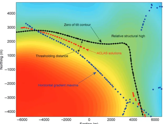
• All the lineaments must be defined as a series of points along either contours or maxima. Each point on each lineament in one set is tested against every nearby point on the other linea-ment set for pairs of points that are within the tolerance dis-tance. Where the points from the two sets of lineaments are within the tolerance distance, the midpoint between the two is chosen as part of the output lineament set (Figure1). The process is repeated for all pairs of nearby points; if the dis-tance between the points is greater than the tolerance, then the midpoint does not contribute to the output lineaments. This process may generate multiple midpoints in a small area, but this is not a problem because they will tend to lie along the average lineament.

• The choice of tolerance distance is important. It must be large enough to produce a coherent output lineament when two input lineaments run adjacent over some distance. It must not, however, be so large that there are spurious coher-ences identified between lineaments that are clearly not re-lated. A practical approach is to start with a small tolerance and gradually increase it for each run until reasonably con-tinuous output lineaments are generated. The tolerance dis-tance should also depend on the character of the gravity or

Figure 1. Illustration of combination of points on individual lineaments to generate ACLAS lineaments. The ACLAS method takes advantage of the deviation between edge-detection methods in the presence of a disrupting source. From the gravity-map derivative (background), it is clear that the edges of the structural high became smoother in the northeast corner. The ACLAS solutions are better suited for geologic fault interpretation than the continuous lines proceeding from single enhancements.

magnetic fields; for lower resolution data or deeper sources, the tolerance distance will necessarily need to be larger.

• Three or more sets of lineaments can be combined based on considering two sets at once. In one approach, coherence is required between every pair of lineament sets. For three sets A, B, and C, the output could be expressed asA∩B∩C, or in practiceðA∩BÞ∩C, such that A and B are compared first and the output is compared with C. Each set of linea-ments has a veto on the output. A larger set of linealinea-ments can be produced by first combining each pair of sets, such that

D¼A∩B;E¼A∩C; andF¼B∩C. The three combi-nations could themselves be combined using the union op-erator∪, where all lineaments from each set are retained, such that the result isD∪E∪F. Thus, any lineament that matches on any two lineament sets will contribute to the ACLAS result.

Calculation of the strike and down-dip direction

The tilt or the vertical derivative of the field can be used to iden-tify the direction of strike of the ACLAS lineaments.Fairhead et al. (2011)show that the direction of fastest descent of the tilt at the zero contour is the direction in which the density or susceptibility de-creases most rapidly. In the case of a simple dip-slip fault and as-suming that density (or magnetization) is increasing with depth, this would generally be the downthrown side of the fault and the perpendicular direction would be the strike direction. An estimate of the dip and strike directions is made at each point along the ACLAS lineaments by taking the direction of fastest descent of the tilt grid; tick marks with this orientation are used at each point to annotate the down-dip direction. Other fields, such as Bouguer gravity or RTP and pseudogravity for magnetics could alternatively be used in this process, but the tilt derivative is generally found to give robust results.

Construction of new lineament chains

Up to this point, the ACLAS lineaments ex-isted purely as a collection of points — calcu-lated as the mean locations of points on coherent original lineaments. In this process, these col-lected points, together with their associated dip values, are collated into chains marking continu-ous features in the data.

The chaining process consists of arranging the solution points in single vectors based on their spatial location. Solution points that are close to each other are considered to belong to the same lineament feature. Points closer to each other than a specified threshold distance are con-nected into lines. A threshold of twice the grid cell size is generally found to be appropriate, but this value needs to be tested in context.

The whole ACLAS method is quick even for large data sets. Comparison and selection of lin-eaments is very fast, less than a minute for 1000 structures, whereas the chaining can take up to 10 min on a standard desktop PC.

APPLICATION TO MODELS

The ACLAS method has been tested on two model data sets; one from a dipping slab model and the other from a synthetic model of a continental margin, both with Gaussian noise added to the magnetic response; both models were developed by Hidalgo-Gato and Bar-bosa (2015).

Slab model

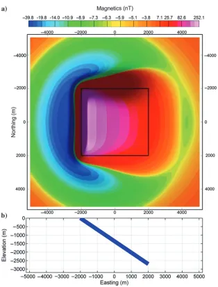
The slab model represents an isolated dipping intrusion (Hidalgo-Gato and Barbosa, 2015), and it is illustrated in Figure 2. The slab is square in map view; it is thin compared with its lateral extent and dips at approximately Figure 2. Slab test model: (a) magnetic anomaly generated by square topped slab and

(b) cross section showing the dip of the slab.

35° to the east. The anomalous magnetic field is calculated based on a vertical ambient field and the slab having vertical induced magnetization with intensity of2 A∕mand no remanent magneti-zation. It should be noted that this model is challenging, and there-fore it is ideal for our purposes because a thin dipping body is not particularly suited to most of the edge-detection methods devel-oped so far and described in the literature. The development of these methods has mostly been based on a model of an infinite contact, which is commonly believed to be a more suitable model for regional structural interpretation.

Maxima of the THD of the magnetic anomaly and maxima of the THD of the tilt were calculated using curvature analysis (Phillips et al., 2007) and combined in ACLAS. For simple 2D model tests, these two edge detectors gave locations on either side of the true position (Pilkington, 2007); this is also observed here with this sim-ple, though not idealized, 3D dipping slab model (Figure3). The ACLAS method takes advantage of this behavior, and the solutions are clearly a better estimate of the 2D position of the edge of the slab than either of the individual sets of solutions (white dots, Figure3a). Combining only lineaments from these two edge detectors, several spurious features not related to the dipping body are still present. When we additionally combine a lineament set derived from zero values of tilt in ACLAS, the spurious solutions are completely elim-inated. The resulting ACLAS solutions show no artifacts and the spatial accuracy is increased (see the comparison of ACLAS

solu-tion with single enhancements in Figure3b). Later, ACLAS solu-tion points were chained into continuous features based on a distance threshold equal to 100 m (two times the cell size; white line, Figure3b). Spurious lineaments have been rejected after inter-secting the early ACLAS solutions with a lineament set derived from zero values of tilt. This secondary application of ACLAS in-troduces a contour method, which is combined with the two maxima-based methods used earlier; as anticipated, this combina-tion is found to be effective in discriminating against spurious lineaments.

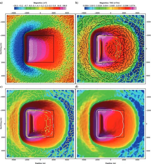
When pseudorandom, zero-mean Gaussian noise with a standard deviation of 10 nT is added to the magnetic response computed from the slab model (Hidalgo-Gato and Barbosa, 2015), picking lineaments becomes more difficult (Figure4). As expected, deriv-atives calculated from the slab-model response corrupted by noise (Figure 4a) are unstable — especially for transformations that include higher order derivatives, such as the THD of the tilt. Deriv-atives have, in fact, been calculated based on a 200 m upward-continued version of the grid; this value is a compromise that reduces noise while limiting the smoothing of anomalies. Even so, the maxima of the THD of the tilt that was effective in the noise-free version of the model, gives a highly complex set of linea-ments (Figure4b), and it is not considered likely to constrain struc-ture location in a useful manner; in fact, ACLAS solutions using this derivative (not shown) were found to be chaotic. Thus, the zero of

Figure 3. The ACLAS results for the slab model without added noise. (a) Tilt THD of the slab-model response. The maxima of the tilt THD are overlaid in black, and the maxima of the THD of the magnetic anomaly are in yellow. The ACLAS-interpolated points are marked in white. (b) Magnetic anomaly overlaid with the maxima of the THD of the tilt (black) and the maxima of the THD of the magnetic anomaly (yellow). Chained ACLAS points (white) were subsequently intersected against zero values of tilt (dashed yellow line) to further remove artifacts.

the tilt was combined with the maxima of the THD of the magnetic anomaly and solutions posted at midpoints to give reasonably coherent ACLAS solutions and more accurately located edges (Fig-ure4cand4d).

It should be noted that, in general, spatial accuracy of retrieved edges is increased, with or without noise added, in compar-ison with results from single enhancements alone (Figures 3 and4).

Figure 4. Slab model magnetic response with added noise. (a) Total field corrupted with 10 nT standard deviation pseudorandom zero-mean Gaussian noise; (b) THD of 200 m upward continued magnetic field overlaid with maxima of THD of upward continued field (yellow) and maxima of tilt THD (black); (c) THD of the upward continued magnetic field overlaid with the maxima of the THD (yellow) and the zero of the tilt (black) with ACLAS lineaments in white; and (d) the chained ACLAS lineaments overlaid on 200 m upward continued field THD.

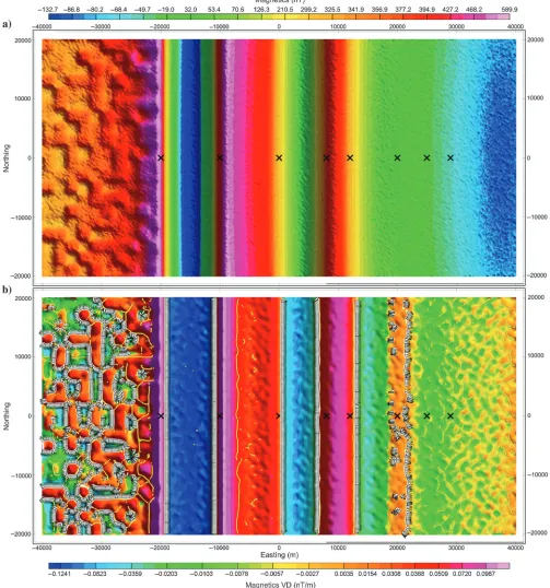
Continental margin model

This model is designed to be a simple but realistic model of a continental margin (Hidalgo-Gato and Barbosa, 2015), and it in-cludes a range of normal and antithetic extensional basement faults (Figure5afterHidalgo-Gato and Barbosa, 2015). In general, faults further east have less displacement and their tops are deeper. The magnetic signal is produced by the basement relief with a vertical ambient field, vertical induced basement magnetization of2 A∕m, and no remanent magnetization; pseudorandom zero-mean Gaussian noise with standard deviation of 10 nT was added to the magnetic field (Figure6a). We apply the same approach tested for the dipping body, and, again, it is found that maxima of THD of magnetic anomaly and zero contour of tilt provide the most coherent lineament sets. These combine into ACLAS lineaments that are very close to the exact location of the faults (black crosses and white lines, Figure6b). Artifacts from both enhancements are removed, and it is seen that for the shallower faults with a larger offset to the west of the grid, ACLAS has produced clean lineaments that match well to the fault locations in the model. The direction of throw is also correctly iden-tified for all delineated faults; however, the smaller, deeper faults fur-ther to the east are not well-imaged. In this area, lineaments from both enhancements are incoherent and match the fault locations less well with some of the faults not being imaged at all.

In general, shallower faults with a bigger offset are resolved most effectively by ACLAS; however, spatial accuracy is also increased for deeper edges. The anomalies of shallower faults are larger and thus have better signal-to-noise ratios, whereas the anomalies re-lated to deeper contacts are affected more by nearby sources. In addition, shallow faults with a large throw are much closer to the infinite contact model, which forms the basis for most of the edge detectors, making them inherently better targets.

ACLAS can reduce artifacts based on the assumption that signals related to the structure should be consistent between lineament sets, whereas noise and artifacts should not. However, if the models that form the basis for the individual lineament algorithms are not ap-propriate in a given situation, then the combined lineaments will be less significant.

In general, both of the models tested are not ideal for the methods that have been applied to them, but coherent ACLAS lineaments have been generated nonetheless. It is observed that for models with noise added, the choice of algorithms to be combined is limited to those that produce reasonably stable results in

their own right: The maxima of the THD of the magnetic anomaly and zero contour of the tilt have worked effectively in both examples.

NORTH WEST AUSTRALIA: APPLICATION TO GRAVITY AND

MAGNETIC GRIDS

To test the effectiveness of the ACLAS method to support the interpretation of large areas, it has been applied to gravity and magnetic grids over part of the Australian North West Shelf. This study area (Figure7) includes a range of structures and includes parts of several geo-logic provinces (Eyles et al., 2001;Gibbons et al., 2012)

• Argo Abyssal Plain: oceanic crust to the north

• Exmouth Plateau: a continental fragment between the Argo Abyssal Plain to the north, the Gascoyne Abyssal Plain to the west, and the Cuvier Abyssal Plain to the southwest

• Pilbara Craton: Archaean cratonic block to the south

• Canning Basin: northwest–southeast-trending Palaeozoic basin to the east.

The area is almost totally covered by good-resolution gravity and magnetic data from Geoscience Australia, so the variability of the data quality is not really a concern. However, the geologic complex-ity, with multiple phases of tectonics, will test how satisfactorily the choices inherent in the ACLAS process can be applied in practice for broad-scale interpretation.

The ACLAS lineaments have been calculated separately for grav-ity (Figures8and9) and magnetic (Figures10and11) grids, based on the Bouguer anomaly (BA) and the RTP magnetic anomaly, re-spectively. Two sets of ACLAS lineaments have been calculated in each case. For gravity, the first is formed from lineaments from the maxima of the THD of BA intersected with lineaments from zero of the tilt of BA (Figure8). This is the combination that was found to be effective for the models, albeit for magnetic data. When plotted on top of the vertical derivative of BA (Figure9), it is apparent that these lineaments (in black) are delineating the main structures across the area. There are, however, some other minor features in the gravity grid and some places where the black lineaments are discontinuous. A second set of ACLAS lineaments was there-fore calculated based on the maxima of the THD of BA intersected with lineaments from the maxima of the THD of tilt of BA. As ob-served earlier with the slab model, this combination is more com-plex than the first set. These lineaments include most of the ACLAS lineaments defined in the first set, but also a large number of other smaller scale lineaments. Some of the additional lineaments mark clear features in the gravity grids; most of these are the lower am-plitude features, often in different directions to the first set of linea-ments, which do not continue for such great distances as for the first set of lineaments. To simplify Figure9, we displayed this second set of lineaments only where the vertical gradient of BA is positive, the implication being that in this case, we are more interested in seg-mentations of structural highs rather than lows. We observed that this second set of lineaments (here referred to as second-order linea-ments) complements the first lineament set and connects across

Figure 5. Continental margin model afterHidalgo-Gato and Barbosa (2015). This is a basement relief model with a vertical ambient field, vertical induced basement magneti-zation of 2 A/m, and no remanent magnetimagneti-zation.

gaps in the first set of lineaments (e.g., the arrow in the central part of Figure9connects a gap probably due to the influence of a lo-cal high).

Based on these observations, it has therefore been decided not to choose between the two sets of ACLAS lineaments, nor to

com-bine them all into one set, but to recognize the first set as“ first-order” lineaments and the second set as “second-order” ments, but only where they do not overlie the first-order linea-ments. Thus, the first-order lineaments appear to define the main structures, whereas the second-order lineaments add some

Figure 6. (a) Magnetic anomaly fromHidalgo-Gato and Barbosa (2015)model with 10 nT standard deviation noise added. Crosses mark the center points of the faults in the model. (b) Tilt of the magnetic anomaly with ACLAS lineaments and dips marked in white.

minor features and fill in some gaps, making the structures more continuous. The filling of gaps in a lineament set is considered to be significant because the segments apparently all form part of a continuous structure, but the gaps in the first-order lineaments are probably due to disturbances from crosscutting structures. This is potentially useful additional information available to the inter-preter by recognizing two sets of lineaments. Overall, the first-and second-order lineaments have fewer of the artifacts that are common in individual lineament sets from a single data-enhance-ment map. It should be noted that the approach described here is not a formula for ideal edge mapping, but it illustrates the type of approaches that can be applied within the ACLAS method to ex-tract lineaments that are robust and applicable to the interpretation needs of a particular area.

First- and second-order ACLAS lineaments have been calcu-lated from the magnetic data in a similar manner (Figures 10 and11). The first-order lineaments (black in Figure 11) are the ACLAS intersection of lineaments from the maxima of the THD of RTP and lineaments from the zero contour of the tilt of RTP. Second-order ACLAS lineaments (gray in Figure 11) are generated from the maxima of the THD of RTP and the maxima of THD of the tilt of RTP. In this case, the second-order lineaments are mostly short features or longer features subparallel to first-order lineaments. These latter might be related to low-am-plitude features, which are too subtle to be seen in the first-order lineament set.

A substantial number of the features match reasonably well be-tween gravity and magnetic results, which is to be expected as the gravity and magnetic data are imaging the same geology, and the aim of the ACLAS process is to discriminate in favor of the most significant lineaments from each data type. These include several longer secondary magnetic lineaments, but overall, they are mostly the intermediate-size features. The smaller, second-order lineaments from the gravity and magnetic data appear mostly to relate to local features that might be described as showing

tex-ture rather than major structex-ture. On the other hand, many of the major gravity anomalies, es-pecially those delineating the boundaries be-tween the geologic provinces, do not correlate with clear linear features from the magnetic data. This relates to the different ways in which geo-logic boundaries are expressed in gravity and magnetic data; in magnetic data, boundaries of geologic provinces are often texture boundaries (as observed in the vertical derivative map, Fig-ure 11), which do not generate strong linear anomalies. The main exception is the boundary between the Pilbara Craton and the Canning Ba-sin, which shows clear lineaments from the grav-ity and magnetic data sets. An interesting case in which a strong magnetic lineament does not cor-relate with gravity lineaments is the north–south first-order magnetic lineament from approxi-mately 121.5E, 18.5S to approxiapproxi-mately 121.5E, 17S (white arrow, Figure11). In fact, this feature appears to correlate with the termination of some west–northwest/east–southeast gravity lin-eaments; this suggests that the magnetic linea-ment is marking a structure that terminates,

offsets, or otherwise interferes with the structures defined by the gravity lineaments. This highlights an important general point with interpretation of automatically generated lineaments, which is that disturbances or terminations of lineaments are often themselves important structural features, possibly delineating strike-slip or wrench faults that are not clearly imaged in their own right because of limited physical property contrast across the faults, along much of their length.

Chained lineaments from gravity and magnetic data are summa-rized in rose diagrams in which in the upper side, we display grav-ity lineaments and in the lower part magnetic lineaments in such a way that when lineaments from the gravity and magnetic data have the same orientation, they are collinear on the diagram; the linea-ment directions are nondirectional, such that north–northwest is considered the same as south–southeast (Figure12). These show the distribution of fault directions for three of the main geologic provinces and give an insight into the prevailing structural con-figurations in the study area. It is interesting to note that the gen-eral distributions in each area are similar for gravity and magnetic lineaments. It can also be seen that the three areas have somewhat different statistics:

• Exmouth Plateau: A strong north–south to north–northeast/ south–southwest to northeast–southwest trend is observed in the rose diagrams (Figure12) and the lineament maps (Fig-ures 9 and 11). This is consistent with the orientation of many prominent geologic features associated with this part of the Northern Carnarvon Basin. These include structures associated with the development, and subsequent reactiva-tion, of the Dampier, Barrow, and Exmouth subbasins, formed when this part of the margin rifted away from India in the early Cretaceous (e.g.,Gibbons et al., 2012). A sec-ondary east–west to west–northwest/east–southeast trend with some very prominent anomalies is also observed. These features may define conduits for the ocean opening to the

Figure 7. Study area on the Australian North West Shelf. Topography/bathymetry with major geologic provinces identified — Argo Abyssal Plain, Exmouth Plateau, Pilbara Block, and Canning Basin.

north (note the significant anomaly separating the Exmouth Plateau from the Argo Abyssal Plain). The north–northeast/ south–southwest lineaments in places, truncate or crosscut the east–west-trending features indicating that the east–west trend is older.

• Canning Basin: The primary lineament orientation observed in both the rose diagrams, and the lineament maps is west– northwest/east–southeast to northwest–southeast consistent with the primary structural trend of the basin. Prominent intrabasin components, such as the Fitzroy Trough, the

Broome Platform, and the Samphire Depression, and asso-ciated structures, are all consistent with the ACLAS deter-mined trend (Cadman et al., 1993). Some of these primary structures are apparently truncated against a north-east–southwest trend, which is also visible as a subtle sec-ondary trend in the rose diagram, possibly related to the rifting away from India event outlined above.

• Pilbara Craton: The dominant lineament orientations are generally less clear in this area with a more chaotic anomaly pattern observed. This is related to the dominance of

high-Figure 8. Gravity data and enhancements used to produce and display the ACLAS lineament map with the coastline (white). (a) Bouguer gravity, (b) vertical derivative, (c) THD, (d) tilt derivative, and (e) THD of tilt.

frequency anomalies from shallow, heterogeneous basement rocks in this ancient, cratonic block.

Overall, the ACLAS lineaments from the gravity and magnetic data provide a valuable input to the first phase structural mapping of the area highlighting the similarities and differences between the informa-tion content of the two data sets. However, these only form a frame-work on which interpretation can be developed; this is best done in a GIS system, together with input from other available data sources.

DISCUSSION

Based on the synthetic models and the Australian North West Shelf example, it appears that the ACLAS method has been success-ful in generating easy-to-read lineament maps with a reduced num-ber of artifacts; indeed, in the synthetic slab case, it is explicitly clear that known artifacts associated with each single enhancement have been cleaned up by ACLAS. From the models with noise, it is apparent that the choice of lineament methods to combine with ACLAS is important. The more stable results tend to be generated from methods in which the order of differentiation is limited; how-ever, real data will not necessarily have excessive acquisition noise as in the synthetic case. The combination of the maxima of the THD of the gravity or magnetic field and the zero of the tilt of the gravity or magnetic field appears generally quite robust. In the real-data example, the addition of ACLAS lineaments from higher order derivatives is seen to add useful information to the resulting linea-ment set. The infilling of broken linealinea-ments is considered helpful, but also diagnostic of crosscutting features and the addition of small-scale features helps to add texture to the interpretation. In these second-order lineaments, there remain some short lineaments that appear incoherent; these could possibly be due to spurious cor-relations of individual lineaments, which do not really correlate from one lineament set to the other, but on occasion they come close enough to be picked by ACLAS.

All examples shown in this paper are combinations of gravity lineaments or combinations of magnetic lineaments, but not combinations of gravity lineaments and magnetic lineaments

to-gether, although there could be correlations between gravity and magnetic lineament sets. The North West Australia example shows that there is a correlation between many gravity and mag-netic ACLAS lineaments, but not all. In general, there are three main reasons that gravity and magnetic lineaments will not match consistently:

1) Acquisition issues: One or another data set may be of low res-olution or anisotropically sampled, such that not all features can be properly imaged. As long as data sets are reasonably well-sampled and the interpretation is not overoptimistic, this should not be a major problem.

2) Susceptibility and density do not correlate: Some geologic boundaries may have a density contrast, but no susceptibility contrast or vice versa. Simple geologic structures may well show similar variations, but boundaries between geologic prov-inces are likely to be complex changes of structural style and texture as well as bulk changes of physical properties. 3) Gravity and magnetic fields image physical property changes in

different ways: Even for simple geologic shapes, the gravity and magnetic anomalies are different.

All these points would need to be considered before attempting to intersect gravity lineaments with magnetic lineaments using ACLAS. The first point should not be a major issue if the data qual-ity is reasonably adequate. The second point is an inevitable effect of geologic complexity, but it would in practice be a major purpose of attempting to find a correlation. The third point can be addressed by choosing appropriate lineament sets. For example, integrating the maxima of the THD of gravity with the maxima of the THD of pseudogravity should provide two lineament sets that correlate with the physical properties in the same way. Possibly, the process of combining gravity and magnetic lineaments with ACLAS will be more stable if it is based on lineament sets that are themselves the output of ACLAS; i.e., only the more coherent gravity features would be correlated with the more coherent magnetic features.

Further developments of the method could include estimation of depths for the ACLAS lineaments. Several methods that

Figure 9. The ACLAS gravity lineaments for the Australian North West Shelf area overlain on ver-tical derivative of the BA. First-order lineaments (black) are generated from the maxima of the THD of BA and the zero of the tilt of BA. Sec-ond-order lineaments (gray) are generated from the maxima of the THD of BA and the maxima of the THD of tilt of BA. Second-order lineaments are only shown where they are complementary to the first-order lineaments. White arrows indicate two places where second-order lineaments help to complete major trends seen in the vertical derivative grid.

generate lineaments can also be used to estimate depths to fea-tures. The attraction of this approach is that the ACLAS linea-ments should consist of only the most robust of the original lineaments and therefore the set of depth solutions should be less contaminated by depths from sections that are themselves spu-rious. For this approach to work in practice and produce depth values along all the lineaments, it is best to use one of the meth-ods that are used to generate the lineaments in the first place. For example, if the zero contour of the tilt or the maxima of the THD of the tilt have been used, then the tilt-depth method (Salem et al., 2007) would be a natural choice that could readily be

imple-mented to assign depths along all the lineaments. For depth es-timation, consideration should be given to the assumptions inherent in the depth-estimation process. As noted previously, many methods assume an infinite depth contact model in their development. In practice, a finite depth-contact model is consid-ered more likely, and thus depths will generally be somewhat underestimated (Flanagan and Bain, 2013;Salem et al., 2013). The extent of the errors will, in practice, depend on the types of structures generating anomalies in the area; this will not nec-essarily be worse than for a general depth-estimation process ap-plied to a large area.

Figure 10. Magnetic data and enhancements used to produce and display the ACLAS lineament map with the coastline (white). (a) The RTP magnetics, (b) vertical derivative, (c) THD, (d) tilt derivative, and (e) THD of tilt.

CONCLUSION

The ACLAS method has largely met its objective of mapping the most reliable edges or lineaments from different edge-detection techniques. The method is fast to implement and execute, and it increases the stability of the edge-detection techniques and the

spa-tial accuracy of the solutions. In addition, it is observed to produce consistent lineaments that are largely free from the typical artifacts seen in standard data enhancements, such as closed contours and multiply branched lineaments. Strike and dip can be calculated automatically, and a clean, coherent set of geologically meaningful lineaments is produced, which can be interpreted with greater con-Figure 12. Rose diagrams showing distribution and length of structural trends for gravity (blue) and magnetic (red) ACLAS lineaments. Three areas are shown separately: (a) Canning Basin, (b) Exmouth Plateau, and (c) Pilbara Block. A very good correlation between the gravity and magnetic structures orientation is observed for the three areas (note: graphs are divided in two in such a way that 0 = 180° orientation).

Figure 11. The ACLAS magnetic lineaments for the Australia North West Shelf area overlain on the vertical derivative of the RTP magnetic anomaly. First-order lineaments (black) are generated from the maxima of the THD of RTP and the zero of the tilt of RTP. Second-order lineaments (gray) are generated from the maxima of the THD of RTP and the maxima of the THD of tilt of RTP. Sec-ond-order lineaments are only shown where they are complementary to the first-order lineaments.

fidence compared with edges or lineaments from standard data en-hancements.

The method is still dependent on the effectiveness of the edge-detection methods used, and ensuring that the choice is appropriate is an important part of the process. It is apparent that the ACLAS method can work effectively in the presence of noise, but the choice of input edge or lineament sets will need to be restricted to those that involve relatively low-order derivatives.

Using different combinations of original lineament sets to gen-erate first- and second-order ACLAS lineaments is seen to be a use-ful approach for real gravity and magnetic data sets. The ability to highlight the continuity of structures and the disturbances along them facilitates the interpretation of dip-slip and strike-slip struc-tures. However, it must be recognized that the ACLAS results are themselves just a tool that needs to be developed into a geologic model together with other available data.

ACKNOWLEDGMENTS

Synthetic magnetic data sets based on models were provided by M. Hidalgo-Gato and V. Barbosa. Gravity and magnetic data sets for Australia have been downloaded from Geoscience Australia and are copyright of the Commonwealth of Australia. We are grateful for constructive comments on a previous version by M. Pilkington, the two unknown reviewers, and associate editor V. Barbosa; they have all helped us to develop the paper. We also want to thank E. Biegert, M. A. Abbas, the unknown reviewers, and the anonymous associate editor for additional constructive comments proposed dur-ing the revision of this version of the paper.

REFERENCES

Blakely, R. J., and R. W. Simpson, 1986, Approximating edges of source bodies from magnetic or gravity anomalies: Geophysics,51, 1494–1498, doi:10.1190/1.1442197.

Cadman, S. J., L. Pain, V. Vuckovic, and S. R. le Poidevin, 1993, Canning Basin, W. A.: Bureau of Resource Sciences, Australian Petroleum Accu-mulations Report 9.

Cooper, G. R. J., and D. R. Cowan, 2006, Enhancing potential field data using filters based on the local phase: Computers and Geosciences,

32, 1585–1591, doi:10.1016/j.cageo.2006.02.016.

Cordell, L. E., and V. J. S. Grauch, 1985, Mapping basement magnetization zones from aeromagnetic data in the San Juan Basin, New Mexico,inW. J. Hinze ed., The utility of regional gravity and magnetic anomaly maps: SEG, 181–197.

Eyles, N., C. H. Eyles, S. N. Apak, and G. M. Carlsen, 2001, Permian-Carboniferous tectono-stratigraphic evolution and petroleum potential of the northern Canning basin, Western Australia: AAPG Bulletin,85, 989–1006.

Fairhead, J. D., A. Salem, L. Cascone, M. Hammill, S. Masterton, and E. Samson, 2011, New developments of the magnetic tilt-depth method to improve structural mapping of sedimentary basins: Geophysical Prospec-ting,59, 1072–1086, doi:10.1111/gpr.2011.59.issue-6.

Fedi, M., 2002, Multiscale derivative analysis: A new tool to enhance gravity source boundaries at various scales: Geophysical Research Letters,29, 16-1–16-4.

Flanagan, G., and J. E. Bain, 2013, Improvements in magnetic depth esti-mation: application of depth and width extent nomographs to standard depth estimation techniques: First Break, 31, 41–51, doi: 10.3997/ 1365-2397.2013028.

Gibbons, A. D., U. Barckhausen, P. van den Bogaard, K. Hoernle, R. Werner, J. M. Whitaker, and R. D. Müller, 2012, Constraining the Jurassic extent of Greater India: Tectonic evolution of the West Australian margin: Geochemistry Geophysics Geosystems, 13, Q05W13, doi: 10.1029/ 2011GC003919.

Hansen, R. O., and E. deRidder, 2006, Linear feature analysis for aeromag-netic data: Geophysics,71, no. 6, L61–L67, doi:10.1190/1.2357831. Hidalgo-Gato, M. C., and V. C. F. Barbosa, 2015, Edge detection of

poten-tial-field sources using scale-space monogenic signal: Fundamental prin-ciples: Geophysics,80, no. 5, J27–J36, doi:10.1190/geo2015-0025.1. McGrath, P. H., 1991, Dip and depth extent of density boundaries using

horizontal derivatives of upward-continued gravity data: Geophysics,

56, 1533–1542, doi:10.1190/1.1442964.

Miller, H. G., and V. Singh, 1994, Potential field tilt—A new concept for location of potential field sources: Journal of Applied Geophysics,32, 213–217, doi:10.1016/0926-9851(94)90022-1.

Nabighian, M. N., 1972, The analytic signal of two dimensional magnetic bodies with polygonal cross-section: Its properties and use for automated anomaly interpretation: Geophysics, 37, 507–517, doi: 10.1190/1 .1440276.

Phillips, J. D., 2000, Locating magnetic contacts: A comparison of the hori-zontal gradient, analytic signal, and local wavenumber methods: 70th An-nual International Meeting, SEG, Expanded Abstracts, 402–405. Phillips, J. D., R. O. Hansen, and R. J. Blakely, 2007, The use of curvature in

potential-field interpretation: Exploration Geophysics,38, 111–119, doi:

10.1071/EG07014.

Pilkington, M., 2007, Locating geological contacts with magnitude trans-forms of magnetic data: Journal of Applied Geophysics, 63, 80–89, doi:10.1016/j.jappgeo.2007.06.001.

Pilkington, M., and P. Keating, 2004, Contact mapping from gridded mag-netic data—A comparison of techniques: Exploration Geophysics,35, 306–311, doi:10.1071/EG04306.

Pilkington, M., and P. Keating, 2010, Geologic applications of magnetic data and using enhancements for contact mapping: Presented at the 72nd An-nual International Conference and Exhibition, EAGE.

Roest, W. R., J. Verhoef, and M. Pilkington, 1992, Magnetic interpretation using the 3-D analytic signal: Geophysics,57, 116–125, doi:10.1190/1 .1443174.

Salem, A., R. Blakely, C. Green, J. D. Fairhead, and D. Ravat, 2014, Es-timation of depth to top of magnetic sources using the local-wavenumber approach in an area of shallow Moho and Curie depth—The Red Sea: Interpretation,2, no. 4, SJ1–SJ8, doi:10.1190/INT-2013-0196.1. Salem, A., S. Campbell, L. Moorhead, and J. D. Fairhead, 2013, An enhanced

tilt depth method for interpreting magnetic data over vertical contacts of finite extent: 75th Annual International Conference and Exhibition, EAGE, Extended Abstracts, doi:10.3997/2214-4609.20130595.

Salem, A., S. E. Williams, J. D. Fairhead, D. Ravat, and R. Smith, 2007, Tilt-depth method: A simple Tilt-depth estimation method using first order mag-netic derivatives: The Leading Edge, 26, 1502–1505, doi: 10.1190/1 .2821934.

Stavrev, P., and D. Gerovska, 2000, Magnetic field transforms with low sensitivity to the direction of source magnetization and high centricity: Geophysical Prospecting,48, 317–340, doi:10.1046/j.1365-2478.2000 .00188.x.

Thurston, J. B., and R. S. Smith, 1997, Automatic conversion of magnetic data to depth, dip, and susceptibility contrast using the SPI method: Geo-physics,62, 807–813, doi:10.1190/1.1444190.

Verduzco, B., J. D. Fairhead, C. M. Green, and C. MacKenzie, 2004, New insights to magnetic derivatives for structural mapping: The Leading Edge,23, 116–119, doi:10.1190/1.1651454.

Wijns, C., C. Perez, and P. Kowalczyk, 2005, Theta map: Edge detection in magnetic data: Geophysics,70, no. 4, L39–L43, doi:10.1190/1.1988184.