behaviour analysis
.
White Rose Research Online URL for this paper:
http://eprints.whiterose.ac.uk/115076/
Version: Published Version
Article:
Isupova, O., Kuzin, D. and Mihaylova, L. (2018) Learning methods for dynamic topic
modeling in automated behaviour analysis. IEEE Transactions on Neural Networks and
Learning Systems, 29 (9). pp. 3980-3993. ISSN 2162-237X
https://doi.org/10.1109/TNNLS.2017.2735364
[email protected] https://eprints.whiterose.ac.uk/
Reuse
This article is distributed under the terms of the Creative Commons Attribution (CC BY) licence. This licence allows you to distribute, remix, tweak, and build upon the work, even commercially, as long as you credit the authors for the original work. More information and the full terms of the licence here:
https://creativecommons.org/licenses/ Takedown
If you consider content in White Rose Research Online to be in breach of UK law, please notify us by
Learning Methods for Dynamic Topic Modeling in
Automated Behavior Analysis
Olga Isupova, Danil Kuzin, and Lyudmila Mihaylova,
Senior Member, IEEE
Abstract— Semisupervised and unsupervised systems provide operators with invaluable support and can tremendously reduce the operators’ load. In the light of the necessity to process large volumes of video data and provide autonomous decisions, this paper proposes new learning algorithms for activity analysis in video. The activities and behaviors are described by a dynamic topic model. Two novel learning algorithms based on the expectation maximization approach and variational Bayes inference are proposed. Theoretical derivations of the posterior estimates of model parameters are given. The designed learning algorithms are compared with the Gibbs sampling inference scheme introduced earlier in the literature. A detailed comparison of the learning algorithms is presented on real video data. We also propose an anomaly localization procedure, elegantly embedded in the topic modeling framework. It is shown that the developed learning algorithms can achieve 95% success rate. The proposed framework can be applied to a number of areas, including transportation systems, security, and surveillance.
Index Terms— Behavior analysis, expectation maximization, learning dynamic topic models, unsupervised learning, varia-tional Bayesian approach, video analytics.
I. INTRODUCTION
B
EHAVIOR analysis is an important area in intelligentvideo surveillance, where abnormal behavior detection is a difficult problem. One of the challenges in this field is informality of the problem formulation. Due to the broad scope of applications and desired objectives, there is no unique way, in which normal or abnormal behavior can be described. In general, the objective is to detect unusual events and inform in due course a human operator about them.This paper considers a probabilistic framework for anomaly detection, where less probable events are labeled as abnormal. We propose two learning algorithms and an anomaly localiza-tion procedure for spatial deteclocaliza-tion of abnormal behaviors.
A. Related Work
There is a wealth of methods for abnormal behavior detection, for example, pattern-based methods [1]–[3]. These
Manuscript received July 28, 2016; revised March 5, 2017; accepted July 25, 2017. Date of publication September 27, 2017; date of current version August 20, 2018. The work of O. Isupova was supported by the EC Seventh Framework Programme [FP7 2013-2017] TRAcking in compleX sensor systems under Grant 607400. The work of L. Mihaylova was supported in part by the EC Seventh Framework Programme [FP7 2013-2017] TRAcking in compleX sensor systems under Grant 607400 and in part by the U.K. Engineering and Physical Sciences Research Council for the support through the Bayesian Tracking and Reasoning over Time under Grant EP/K021516/1.
(Corresponding author: Olga Isupova.)
The authors are with the Department of Automatic Control and Sys-tems Engineering, University of Sheffield, Sheffield S10 2TN, U.K. (e-mail: [email protected]; [email protected]; l.s.mihaylova@ sheffield.ac.uk).
Color versions of one or more of the figures in this paper are available online at http://ieeexplore.ieee.org.
Digital Object Identifier 10.1109/TNNLS.2017.2735364
methods extract explicit patterns from data and use them as behavior templates for decision-making. In [1], the sum of the visual features of a reference frame is treated as a normal behavior template. Another common approach for representing normal templates is using clusters of visual features [2], [3]. Visual features can range from raw intensity values of pixels to complex features that exploit the data nature [4].
In the testing stage, new observations are compared with the extracted patterns. The comparison is based on some similarity measure between observations, e.g., the
Jensen–Shannon divergence in [5] or the Z-score value in [2]
and [3]. If the distance between the new observation and any of the normal patterns is larger than a threshold, then the observation is classified as abnormal.
Abnormal behavior detection can be considered as a clas-sification problem. It is difficult in advance to collect and label all kind of abnormalities. Therefore, only one-class label can be expected and one-class classifiers are applied to abnormal behavior detection, e.g., a one-class support vector machine [6], a support vector data description algorithm [7], a neural network approach [8], and a level set method [9] for normal data boundary determination [10].
Another class of methods relies on the estimation of probability distributions of the visual data. These estimated distributions are then used in the decision-making process. Different kinds of probability estimation algorithms are pro-posed in the literature, e.g., based on nonparametric sample histograms [11], Gaussian distribution modeling [12]. Spatio-temporal motion data dependence is modeled as a coupled Hidden Markov Model (HMM) in [13]. Autoregressive process modeling based on self-organized maps is proposed in [14].
An efficient approach is to seek for feature sets that tend to appear together. These feature sets form typical activi-ties or behaviors in the scene. Topic modeling [15], [16] is an approach to find such kinds of statistical regularities in a form of probability distributions. The approach can be applied for abnormal behavior detection (see [17]–[19]). A number of variations of the conventional topic models for abnormal behavior detection have been recently proposed: clustering of activity distributions [20]; modeling temporal dependencies among activities [21]; and a continuous model for an object velocity [22].
Within the probabilistic modeling approach [12], [13], [17], [18], [20], [22] the decision about abnormality is mainly made by computing likelihood of a new observation. The comparison of the different abnormality measures based on the likelihood estimation is provided in [19].
Topic modeling is originally developed for text
mining [15], [16]. It aims to find latent variables called
“topics” given the collection of unlabeled text documents
consisted ofwords. In probabilistic topic modeling documents
are represented as a mixture of topics, where each topic is assumed to be a distribution over words.
There are two main types of topic models: probabilistic latent semantic analysis (PLSA) [15] and latent Dirichlet allo-cation (LDA) [16]. The former considers the problem from the frequentist perspective, while the later studies it within the Bayesian approach. The main learning techniques proposed for these models include maximum likelihood estimation via the Expectation–Maximization (EM) algorithm [15], variational Bayes (VB) inference [16], Gibbs sampling (GS) [23], and maximum a posteriori (MAP) estimation [24].
B. Contributions
In this paper, inspired by ideas from [21], we propose an unsupervised learning framework based on a Markov Clustering Topic Model (MCTM) for behavior analysis and anomaly detection. It groups possible topic mixtures of visual documents and forms a Markov chain for the groups.
The key contributions of this paper consist in developing new learning algorithms, namely MAP estimation using the EM algorithm and VB inference for the MCTM, and in proposing an anomaly localization procedure that follows con-cepts of probabilistic topic modeling. We derive the likelihood expressions as a normality measure of newly observed data. The developed learning algorithms are compared with the GS scheme proposed in [21]. A comprehensive analysis of the algorithms is presented over real video sequences. The empirical results show that the proposed methods provide more accurate results than the GS scheme in terms of anomaly detection performance.
Our preliminary results with the EM algorithm for behavior analysis are published in [25]. In contrast to [25] we now consider a fully Bayesian framework, where we propose the EM algorithm for MAP estimates rather than the maximum likelihood ones. We also propose here a novel learning algo-rithm based on VB inference and a novel anomaly localization procedure. The experiments are performed on more challeng-ing data sets in comparison to [25].
The rest of this paper is organized as follows. Section II describes the overall structure of visual documents and visual words. Section III introduces the dynamic topic model. The new learning algorithms are presented in Section IV, where the proposed MAP estimation via the EM algorithm and VB algorithm are introduced first and then the GS scheme is reviewed. The methods are given with a detailed discussion about their similarities and differences. The anomaly detection procedure is presented in Section V. The learning algorithms are evaluated with real data in Section VI, and Section VII concludes this paper.
II. VIDEOANALYTICSWITHIN THETOPIC
MODELINGFRAMEWORK
Video analytics tasks can be formulated within the frame-work of topics modeling. This requires a definition of visual documents and visual words (see [20], [21]). The whole video sequence is divided into nonoverlapping short clips. These clips are treated as visual documents. Each frame is divided next into grid cells of pixels. Motion detection is applied to each of the cells. The cells where motion is detected are called moving cells. For each of the moving cells the motion direction is determined. This direction is further quantized into four dominant ones—up, left, down, and right (see Fig. 1). The position of the moving cell and the quantized direction of its motion form a visual word.
Fig. 1. Structure of the visual feature extraction. From an input frame (left), a map of local motions is calculated (center). The motion is quantized into four directions to get the feature representation (right).
Each of the visual documents is then represented as a sequence of visual words’ identifiers, where identifiers are obtained by some ordering of a set of unique words. This discrete representation of the input data can be processed by topic modeling methods.
III. MARKOVCLUSTERINGTOPICMODEL FOR
BEHAVIORALANALYSIS
A. Motivation
In topic modeling, there are two main kinds of distributions—the distributions over words, which correspond to topics, and the distributions over topics, which charac-terize the documents. The relationship between documents and words is then represented via latent low-dimensional entities called topics. Having only an unlabeled collection of documents, topic modeling methods restore a hidden structure of data, i.e., the distributions over words and the distributions over topics.
Consider a set of distributions over topics and a topic distribution for each document is chosen from this set. If the cardinality of the set of distributions over topics is less than the number of documents, then documents are clustered into groups such that documents have the same topic distribution within a group. A unique distribution over topics is called a behavior in this paper. Therefore, each document
corre-sponds to one behavior. In topic modeling, a document is fully described by a corresponding distribution over topics, which means in this case a document is fully described by a corresponding behavior.
There are a number of applications where we can observe documents clustered into groups with the same distribution over topics. Let us consider some examples from video ana-lytics where a visual word corresponds to a motion within a tiny cell. As topics represent words that statistically often appear together, in video analytics applications topics define some motion patterns in local areas.
Let us consider a road junction regulated by traffic lights. A general motion on the junction is the same with the same traffic light regime. Therefore, the documents associated with the same traffic light regimes have the same distributions over topics, i.e., they correspond to the same behaviors.
[image:3.612.330.548.64.142.2]Each action in real life lasts for some time, e.g., a traffic light regime stays the same and people get on and off a train for several seconds. Moreover, often these different types of motion or behaviors follow a cycle and their changes occur in some order. These insights motivate to model a sequence of behaviors as a Markov chain, so that the behaviors remain the same during some documents and change in a predefined order. The model that has these described properties is called an MCTM in [21]. The next section formally formulates the model.
B. Model Formulation
This section starts from the introduction of the main
nota-tions used through this paper. Denote by X the vocabulary
of all visual words, by Y the set of all topics, byZ the set
of all behaviors, and x, y, and z are used for elements from
these sets, respectively. When an additional element of a set is required, it is denoted with a prime, e.g.,z′is another element
from Z.
Let xt = {xi,t}Ni=t1 be a set of words for the document t, where Nt is the length of the documentt. Letx1:Ttr = {xt}
Ttr t=1
denote a set of all words for the whole data set, where Ttr
is the number of documents in the data set. Similarly, denote by yt = {yi,t}iN=t1 andy1:Ttr = {yt}
Ttr
t=1 a set of topics for the
document t and a set of all topics for the whole data set,
respectively. Let z1:Ttr = {zt} Ttr
t=1be a set of all behaviors for
all documents.
Note that x, y, and z without subscript denote possible
values for a word, topic, and behavior from X, Y, and Z,
respectively, while the symbols with subscript denote word, topic, and behavior assignments in particular places in a data set.
Here, is a matrix corresponding to the distributions
over words given the topics, is a matrix
correspond-ing to the distributions over topics given behaviors. For
a Markov chain of behaviors, a vector π for a
behav-ior distribution for the first document and a matrix for
transition probability distributions between the behaviors are introduced
= {φx,y}x∈X,y∈Y, φx,y =p(x|y), φy = {φx,y}x∈X = {θy,z}y∈Y,z∈Z, θy,z= p(y|z), θz = {θy,z}y∈Y
π = {πz}z∈Z, πz = p(z)
= {ξz′,z}z′∈Z,z∈Z, ξz′,z= p(z′|z), ξz = {ξz′,z}z′∈Z
where the matrices , , and and the vector π are
formed as follows. An element of a matrix on the ith row
and jth column is a probability of the ith element given
the jth one, e.g., φx,y is a probability of the word x in the topic y. The columns of the matrices are then distributions for
corresponding elements, e.g., θz is a distribution over topics for the behavior z. Elements of the vectorπ are probabilities
of behaviors to be chosen by the first document. All these distributions are categorical.
The introduced distributions form a set
= {,,π,} (1)
of model parameters, and they are estimated during a learning procedure.
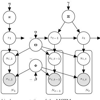
Fig. 2. Graphical representation of the MCTM.
Prior distributions are imposed to all the parameters. Conjugate Dirichlet distributions are used
φy ∼Dir(φy|β), ∀y∈Y
θz ∼Dir(θz|α), ∀z∈Z
π ∼Dir(π|η)
ξz ∼Dir(ξz|γ), ∀z∈Z
where Dir(·)is a Dirichlet distribution andβ,α,η, andγ are
the corresponding hyperparameters. As topics and behaviors are not known a priori and will be specified via the learning procedure, it is impossible to distinguish two topics or two behaviors in advance. This is the reason why all the prior distributions are the same for all topics and all behaviors.
The generative process for the model is as follows. All the parameters are drawn from the corresponding prior Dirichlet distributions. At each time momentt, a behaviorzt is chosen first for a visual document. The behavior is sampled using the
matrix according to the behavior chosen for the previous
document. For the first document, the behavior is sampled using the vector π.
Once the behavior is selected, the procedure of choosing visual words repeats for the number of times equal to the length of the current documentNt. The procedure consists of two steps—sampling a topicyi,t using the matrixaccording to the chosen behavior zt followed by sampling a word xi,t using the matrixaccording to the chosen topicyi,t for each token i ∈ {1, . . . ,Nt}, where a token is a particular place inside a document where a word is assigned. The generative process is summarized in Algorithm 1. The graphical model, showing the relationships between the variables, can be found in Fig. 2.
The full likelihood of the observed variablesx1:Ttr, the
hid-den variablesy1:Ttr andz1:Ttr, and the set of parameters can
be written then as follows:
p(x1:Ttr,y1:Ttr,z1:Ttr, |β,α,η,γ)
= p(π|η)p(|γ)p(|α)p(|β)
Priors
×p(z1|π)
Ttr
t=2
p(zt|zt−1,) Ttr
t=1
Nt
i=1
p(xi,t|yi,t,)p(yi,t|zt,)
Likelihood
.
[image:4.612.355.517.55.216.2]Algorithm 1 Generative Process for the MCTM
Require: The number of clips – Ttr, the length of each clip – Nt ∀t = {1, . . . ,Ttr}, the hyperparameters –β,α,η,γ;
Ensure: The data setx1:Ttr = {x1,1, . . . ,xi,t, . . . ,xNTtr,Ttr};
1: for all y∈Y do
2: draw a word distribution for the topicy:
φy ∼Dir(φy|β);
3: for all z∈Z do
4: draw a topic distribution for behaviorz:
θz ∼Dir(θz|α);
5: draw a transition distribution for behaviorz:
ξz ∼Dir(ξz|γ);
6: draw a behavior probability distribution for the initial
document
π ∼Dir(φ|η);
7: for all t∈ {1, . . . ,Ttr}do
8: if t =1 then
9: draw a behavior for the document from the initial
distribution: zt ∼Cat(zt|π)1;
10: else
11: draw a behavior for the document based on the
behav-ior of the previous document:zt ∼Cat(zt|ξzt−1); 12: for alli ∈ {1, . . . ,Nt}do
13: draw a topic for the token i based on the chosen
behavior: yi,t ∼Cat(yi,t|θzt);
14: draw a visual word for the tokeni based on the chosen
topic: xi,t ∼Cat(xi,t|φyi,t);
an EM algorithm for the MAP estimates of the parameters and based on VB inference to estimate posterior distributions of the parameters. We introduce the proposed learning algorithms below and briefly reviewed the GS scheme.
IV. PARAMETERSLEARNING
A. Learning: EM Algorithm Scheme
We propose a learning algorithm for MAP estimates of the parameters based on the EM algorithm [26]. The algorithm consists of repeating E- and M-steps. Conventionally, the EM algorithm is applied to get maximum likelihood estimates. In that case, the M-step is
Q( , old)−→max (3)
where old denotes the set of parameters obtained at the
previous iteration, and Q( , old) is the expected logarithm
of the full likelihood function of the observed and hidden variables
Q( , old)
=Ep(y1:Ttr,z1:Ttr|x1:Ttr, old)logp(x1:Ttr,y1:Ttr,z1:Ttr| ). (4)
1Here,Cat(·|v)denotes a categorical distribution, where components of a vectorvare probabilities of a discrete random variable to take one of possible
values.
The subscript of the expectation sign means the distribu-tion, with respect to which the expectation is calculated. During the E-step, the posterior distribution of the hidden variables is estimated given the current estimates of the parameters.
In this paper, the EM algorithm is applied to get MAP estimates instead of traditional maximum likelihood ones. The M-step is modified in this case as
Q( , old)+logp( |β,α,η,γ)−→max (5)
where p( |β,α,η,γ)is the prior distribution of the parame-ters.
As the hidden variables are discrete, the expectation con-verts to a sum of all possible values for the whole set of the hidden variables {y1:Ttr,z1:Ttr}. The substitution of the
likelihood expression from (2) into (5) allows to marginalize some hidden variables from the sum. The remaining
distrib-utions that are required for computing theQ-function are as
follows:
• p(z1 = z|x1:Ttr,
old)—the posterior distribution of a
behavior for the first document;
• p(zt =z′,zt−1 =z|x1:Ttr,
old)—the posterior
distribu-tion of two behaviors for successive documents;
• p(yi,t = y|x1:Ttr,
old)—the posterior distribution of a
topic assignment for a given token;
• p(yi,t = y,zt = z|x1:Ttr,
old)—the joint posterior
distribution of a topic and behavior assignments for a given token.
With the fixed current values for these posterior distributions the estimates of the parameters that maximize the required functional of the M-step (5) can be computed as
φxEM,y =
βx+ ˆnxEM,y −1
+
x′∈X
βx′+ ˆnxEM′,y−1
+
, ∀x∈X, y∈Y (6)
θyEM,z =
αy+ ˆnyEM,z −1
+
y′∈Y
αy′+ ˆnEM y′,z−1
+
, ∀y∈Y, z∈Z (7)
ξzEM′,z =
γz′+ ˆnEM z′,z −1
+
ˇ
z∈Z
γzˇ+ ˆnzˇEM,z −1
+
, ∀z′, z∈Z (8)
πzEM=
ηz+ ˆnzEM−1
+
z′∈Z
ηz′ + ˆnEM z′ −1
+
, ∀z∈Z (9)
where(a)+def=max(a,0)[27];βx,αy, andγz′ are the elements
of the hyperparameter vectors β, α, and γ, respectively;
ˆ
nxEM,y = Ttr
t=1iN=t1p(yi,t = y|x1:Ttr,
old)I(x
i,t = x)is the
expected number of times, when the word x is associated
with the topic y, whereI(·)is the indicator function;nˆyEM,z =
Ttr
t=1iN=t1p(yi,t = y,zt = z|x1:Ttr, old) is the expected
number of times, when the topic y is associated with the
behavior z; nˆzEM = p(z1 = z|x1:Ttr, old) is the “expected
number of times,” when the behaviorz is associated with the
first document, in this case the “expected number” is just a probability, the notation is used for the similarity with the rest of the parameters; and nˆzEM′,z =Tt=tr2p(zt = z′,zt−1 = z|x1:Ttr,
old) is the expected number of times, when the
behaviorz is followed by the behavior z′.
During the E-step with the fixed current estimates of the
parameters old, the updated values for the posterior
derivation of the updated formulas for these distributions is similar to the Baum–Welch forward–backward algorithm [28], where the EM algorithm is applied to the maximum likelihood estimates for a HMM. This similarity appears because the generative model can be viewed as extension of a HMM.
For effective computation of the required posterior distri-butions, the additional variables α´z(t) and β´z(t) are intro-duced. A dynamic programming technique is applied for computation of these variables. Having the updated values for α´z(t) and β´z(t), one can update the required posterior distributions of the hidden variables. The E-step is then formulated as follows (for simplification of notation the super-script “old” for the parameters variables is omitted inside the formulas): ⎧ ⎪ ⎪ ⎪ ⎪ ⎪ ⎪ ⎪ ⎪ ⎪ ⎨ ⎪ ⎪ ⎪ ⎪ ⎪ ⎪ ⎪ ⎪ ⎪ ⎩ ´ αz(t)=
Nt
i=1
y∈Y
φxi,t,yθy,z
×
z′∈Z
´
αz′(t−1)ξz,˜z, if t ≥2
´
αz(1)=πz N1
i=1
y∈Y
φxi,1,yθy,z
(10) ⎧ ⎪ ⎪ ⎪ ⎪ ⎪ ⎪ ⎨ ⎪ ⎪ ⎪ ⎪ ⎪ ⎪ ⎩ ´ βz(t)=
z′∈Z
´
βz′(t+1)ξz′,z
× Nt+1
i=1
y∈Y
φxi,t+1,yθy,z′, ift <Ttr
´
βz(Ttr)=1
(11)
K = z∈Z
´
αz(1)β´z(1) (12)
p(z1|x1:Ttr,
old)= α´z1(1)β´z1(1)
K (13)
p(zt,zt−1|x1:Ttr,
old)= α´zt−1(t−1)β´zt(t)ξzt,zt−1 K
× Nt
i=1
y∈Y
φxi,t,yθy,zt (14)
⎧ ⎪ ⎪ ⎪ ⎪ ⎪ ⎪ ⎪ ⎪ ⎪ ⎪ ⎪ ⎪ ⎪ ⎪ ⎪ ⎪ ⎨ ⎪ ⎪ ⎪ ⎪ ⎪ ⎪ ⎪ ⎪ ⎪ ⎪ ⎪ ⎪ ⎪ ⎪ ⎪ ⎪ ⎩
p(yi,t,zt|x1:Ttr,
old)= φxi,t,yi,tθyi,t,ztβ´zt(t)
K
×
z′∈Z
´
αz′(t−1)ξz t,z′
Nt
j=1
j=i
y′∈Y
φxj,t,y′θy′,zt, if t≥2
p(yi,1,z1|x1:Ttr, old)=
φxi,1,yi,1θyi,1,z1β´z1(1) K
×πz1
N1
j=1
j=i
y′∈Y
φxj,1,y′θy′,z
1
(15)
p(yi,t|x1:Ttr,
old)=
z∈Z
p(yi,t,z|x1:Ttr,
old) (16)
where K is a normalization constant for all the posterior
distributions of the hidden variables.
Starting with some random initialization of the parameter estimates, the EM algorithm iterates the E- and M-steps until convergence. The obtained estimates of the parameters are used for further analysis.
B. Learning: Variational Bayes Scheme
We also propose a learning algorithm based on the VB approach [29] to find approximated posterior distributions for both the hidden variables and the parameters.
In the VB inference scheme, the true posterior distribution, in this case the distribution of the parameters and the hidden variables p(y1:Ttr,z1:Ttr, |x1:Ttr,η,γ,α,β), is approximated
with a factorized distribution—q(y1:Ttr,z1:Ttr, ). The
approx-imation is made to minimize the Kullback–Leibler divergence between the factorized distribution and true one. We factorize the distribution in order to separate the hidden variables and the parameters
ˆ
q(y1:Ttr,z1:Ttr, )
= ˆq(y1:Ttr,z1:Ttr)qˆ( )
def
= argmin KL(q(y1:Ttr,z1:Ttr)q( )||
p(y1:Ttr,z1:Ttr, |x1:Ttr,η,γ,α,β)) (17)
where KL denotes the Kullback–Leibler divergence. The min-imization of the Kullback–Leibler divergence is equivalent to the maximization of the evidence lower bound. The maximiza-tion is done by coordinate ascent [29].
During the update of the parameters, the approximated distributionq( )is further factorized
q( )=q(π)q()q()q(). (18) Note that this factorization of approximated parameter distributions is a corollary of our model and not an assumption.
The iterative process of updating the approximated dis-tributions of the parameters and the hidden variables can be formulated as an EM-like algorithm, where during the E-step, the approximated distributions of the hidden variables are updated and during the M-step, the approximated distrib-utions of the parameters are updated.
The M-like step is as follows:
⎧ ⎨ ⎩
q()= y∈Y
Dir(φy; ˜βy)
˜
βx,y =βx+ ˆnxVB,y, ∀x∈X,y∈Y
(19)
⎧ ⎨ ⎩
q()= z∈Z
Dir(θz; ˜αz)
˜
αy,z =αy+ ˆnyVB,z, ∀y∈Y,z∈Z
(20)
q(π)=Dir(π; ˜η) ˜
ηz =ηz+ ˆnzVB, ∀z∈Z
(21)
⎧ ⎨ ⎩
q()= z∈Z
Dir(ξz; ˜γz)
˜
γz′,z =γz′ + ˆnVB
z′,z, ∀z′,z∈Z
(22)
whereβ˜
y,α˜z, η˜, andγ˜z are updated hyperparameters of the corresponding posterior Dirichlet distributions, and nˆxVB,y =
Ttr
t=1iN=t1I(xi,t =x)q(yi,t =y)is the expected number of times, when the wordxis associated with the topicy. Here and
below the expected number is computed with respect to the approximated posterior distributions of the hidden variables;
ˆ
nyVB,z =Ttr t=1
Nt
i=1q(yi,t =y,zt =z)is the expected number of times, when the topic y is associated with the behavior z;
ˆ
nzVB = q(z1 = z) is the “expected number” of times,
and nˆzVB′,z =
Ttr
t=2q(zt = z′,zt−1 = z) is the expected
number of times, when the behavior z is followed by the
behavior z′.
The following additional variables are introduced for the E-like step:
˜
πz =exp
⎛
⎝ψ(η˜z)−ψ
⎛
⎝
z′∈Z
˜ ηz′
⎞ ⎠
⎞
⎠ (23)
˜
ξ˜z,z =exp
⎛
⎝ψ(γ˜z˜,z)−ψ
⎛
⎝
z′∈Z
˜ γz′,z
⎞ ⎠ ⎞
⎠ (24)
˜
φx,y =exp
ψ(β˜x,y)−ψ
x′∈X
˜ βx′,y
(25)
˜
θy,z =exp
⎛
⎝ψ(α˜y,z)−ψ
⎛
⎝
y′∈Y
˜ αy′,z
⎞ ⎠ ⎞
⎠ (26)
whereψ(·)is the digamma function.
Using these additional notations, the E-like step is formu-lated the same as the E-step of the EM algorithm, replac-ing everywhere the estimates of the parameters with the corresponding tilde introduced notation and true posterior distributions of the hidden variables with the corresponding approximated ones in (10)–(16).
The point estimates of the parameters can be obtained by expected values of the posterior approximated distributions. An expected value for a Dirichlet distribution (a posterior distribution for all the parameters) is a normalized vector of hyperparameters. Using the expressions for the hyperparame-ters from (19)–(22), the final paramehyperparame-ters’ estimates can be obtained by
φxVB,y = βx+ ˆn
VB
x,y
x′∈X
βx′+ ˆnVB x′,y
, ∀x∈X,y∈Y (27)
θyVB,z = αy+ ˆn
VB
y,z
y′∈Y
αy′+ ˆnyVB′,z
, ∀y∈Y,z∈Z (28)
ξzVB′,z =
γz′+ ˆnVB z′,z
ˇ
z∈Z
γˇz+ ˆnˇzVB,z
, ∀z′,z∈Z (29)
πzVB = ηz + ˆn
VB
z
z′∈Z
ηz′+ ˆnVB z′
, ∀z∈Z. (30)
C. Learning: Gibbs Sampling Algorithm
In [21], the collapsed version of GS is used for parameter learning in the MCTM. The Markov chain is built to sample only the hidden variables yi,t and zt, while the parameters
,, andare integrated out (note that the distribution for
the initial behavior choice π is not considered in [21]).
During the burn-in stage, the hidden topic and behav-ior assignments to each token in the data set are drawn from the conditional distributions given all the remaining variables. Following the Markov Chain Monte Carlo frame-work, it would draw samples from the posterior distribution
p(y1:Ttr,z1:Ttr|x1:Ttr,β,α,η,γ). From the whole sample for
{y1:Ttr,z1:Ttr}, the parameters can be estimated as in [23] φxGS,y = nˆ
GS
x,y+βx
x′∈XnˆxGS′,y+βx′
, ∀x ∈X,y∈Y (31)
θyGS,z = nˆ
GS
y,z +αy
y′∈Y
ˆ
nyGS′,z+αy′
, ∀y∈Y,z∈Z (32)
ξzGS′,z =
ˆ
nzGS′,z+γz′
ˇ
z∈Z
ˆ
nzˇGS,z +γˇz
, ∀z′,z∈Z (33)
where nˆxGS,y is the count for the number of times, when the word x is associated with the topic y; nˆyGS,z is the count for the topic y and the behavior z pair; nˆzGS′,z is the count for
the number of times, when the behavior z is followed by the
behaviorz′.
D. Similarities and Differences of the Learning Algorithms
The point parameter estimates for all three learning algo-rithms (6)–(9), (27)–(30), and (31)–(33) have a similar form. The EM algorithm estimates differ up to the hyperparameters reassignment—adding one to all the hyperparameters in the VB or GS algorithms ends up with the same final equations for the parameters estimates in the EM algorithm. We explore this in the experimental part. This “-1” term in the EM algo-rithm formulas (6)–(8) occurs because it uses modes of the posterior distributions, while the point estimates obtained by the VB and GS algorithms are means of the corresponding posterior distributions. For a Dirichlet distribution, which is a posterior distribution for all the parameters, mode and mean expressions differ by this “-1” term.
The main differences of the methods consist in the ways the countsnx,y,ny,z, andnz′,z are estimated. In the GS algorithm,
they are calculated by a single sample from the posterior dis-tribution of the hidden variablesp(y1:Ttr,z1:Ttr|x1:Ttr,β,α,γ).
In the EM algorithm, the counts are computed as expected numbers of the corresponding events with respect to the posterior distributions of the hidden variables. In the VB algo-rithm, the counts are computed in the same way as in the EM algorithm up to replacing the true posterior distributions with the approximated ones.
Our observations for the dynamic topic model confirm the comparison results for the vanilla PLSA and LDA models provided in [30].
V. ANOMALYDETECTION
This paper presents on-line anomaly detection with the MCTM in video streams. The decision-making procedure is divided into two stages. At a learning stage, the parameters are
estimated using Ttr visual documents by one of the learning
algorithms, presented in Section IV. After that during a testing stage a decision about abnormality of new upcoming testing documents is made comparing a marginal likelihood of each document with a threshold. The likelihood is computed using the parameters obtained during the learning stage. The thresh-old is a parameter of the method and can be set empirically, for example, to label 2% of the testing data as abnormal. This paper presents a comparison of the algorithms (Section VI) using the measure independent of threshold value selection.
information about anomalies, while documents labeled as abnormal provide temporal detection. The following sections introduce both the anomaly detection procedure on a document level and the anomaly localization procedure within a video frame.
A. Abnormal Documents Detection
The marginal likelihood of a new visual document xt+1
given all the previous data x1:t can be used as a normality measure of the document [21]
p(xt+1|x1:t) =
p(xt+1|x1:t,,,)p(,,|x1:t)ddd. (34) If the likelihood value is small it means that the current document cannot be fit to the learnt behaviors and topics, which represent typical motion patterns. Therefore, this is an indication for an abnormal event in this document. The decision about abnormality of a document is then made by comparing the marginal likelihood of the document with the threshold.
In real world applications, it is essential to detect anomalies as soon as possible. Hence an approximation of the integral in (34) is used for efficient computation. The first approxi-mation is based on the assumption that the training data set is representative for parameter learning, which means that the posterior probability of the parameters would not change if there is more observed data
p(,,|x1:t)≈ p(,,|x1:T r) ∀t ≥Ttr. (35) The marginal likelihood can be then approximated as
p(xt+1|x1:t,,,)p(,,|x1:t)ddd ≈
p(xt+1|x1:t,,,)p(,,|x1:Ttr)ddd.
(36) Depending on the algorithm used for learning the integral in (36) can be further approximated in different ways. We con-sider two types of approximation.
1) Plug-in Approximation: The point estimates of the
para-meters can be plug-in in the integral (36) for approximation
p(xt+1|x1:t,,,)p(,,|x1:T r)ddd ≈
p(xt+1|x1:t,,,)δˆ()δˆ(), δˆ()ddd
= p(xt+1|x1:t,ˆ,ˆ,ˆ) (37) whereδa(·)is the delta-function with the center ina;ˆ,ˆ,ˆ are point estimates of the parameters, which can be computed by any of the considered learning algorithms using (6)–(8), (27)–(29), or (31)–(33).
The product and sum rules, the conditional independence equations from the generative model are then applied and the final formula for the plug-in approximation is as follows:
p(xt+1|x1:t)≈ p(xt+1|x1:t,ˆ,ˆ,ˆ)
=
zt
zt+1
[p(xt+1|zt+1,ˆ,ˆ)p(zt+1|zt,ˆ) ×p(zt|x1:t,ˆ,ˆ,ˆ)] (38)
where the predictive probability of the behavior for the current document, given the observed data up to the current document, can be computed via the recursive formula
p(zt|x1:t,ˆ,ˆ,ˆ)
=
zt−1
p(xt|zt,ˆ,ˆ)p(zt|zt−1,ˆ)p(zt−1|x1:t−1,ˆ,ˆ,ˆ) p(xt|x1:t−1,ˆ,ˆ,ˆ)
.
(39)
The point estimates can be computed for all three learning algorithms; therefore, a normality measure based on the plug-in approximation of the margplug-inal likelihood is applicable for all of them.
2) Monte Carlo Approximation: If samples {s,s,s} from the posterior distribution p(,,|x1:Ttr)of the
para-meters can be obtained, the integral (36) is further approxi-mated by the Monte Carlo method
p(xt+1|x1:t,,,)p(,,|x1:Ttr)ddd
≈ 1
S
S
s=1
p(xt+1|x1:t,s,s,s) (40)
where S is the number of samples. These samples can
be obtained: 1) from the approximated posterior distribu-tions q(), q(), and q() of the parameters, computed by the VB learning algorithm or 2) from the independent samples of the GS scheme. For the conditional likelihood
p(xt+1|x1:t,s,s,s), the formula (38) is valid.
Note that for the approximated posterior distribution of the parameters, i.e., the output of the VB learning algorithm, the integral (36) can be resolved analytically, but it would be computationally infeasible. This is the reason why the Monte Carlo approximation is used in this case.
Finally, in order to compare documents of different lengths
the normalized likelihood is used as a normality measures
s(xt+1)= 1
Nt+1p(xt+1|x1:t). (41)
B. Localization of Anomalies
The topic modeling approach allows to compute a likelihood function not only of the whole document but of an individual word within the document too. Recall that the visual word contains the information about a location in the frame. We pro-pose to use the location information from the least probable words (e.g., 10 words with the least likelihood values) to localize anomalies in the frame. Note, we do not require anything additional to a topic model, e.g., modeling regional information explicitly as in [31] or comparing a test document with training ones as in [32]. Instead, the proposed anomaly localization procedure is general and can be applied in any topic modeling-based method, where spatial information is encoded to visual words.
The marginal likelihood of a word can be computed in a similar way to the likelihood of the whole document. For the point estimates of the parameters and plug-in approximation of the integral, it is
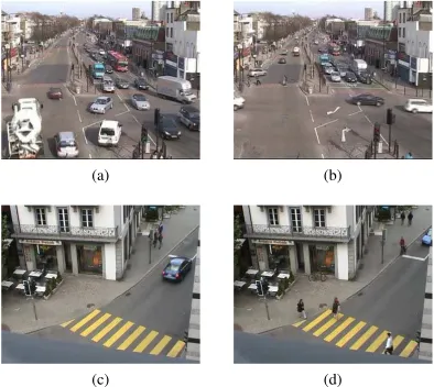
Fig. 3. Sample frames of the real data sets. (a) and (b) Two sample frames from the QMUL data. (c) and (d) Two sample frames from the Idiap data.
For the samples from the posterior distributions of the para-meters and the Monte Carlo integral approximation, it is
p(xi,t+1|x1:t)≈ 1
S
S
s=1
p(xi,t+1|x1:t,s,s,s). (43)
VI. PERFORMANCEVALIDATION
We compare the two proposed learning algorithms, based on EM and VB, with the GS algorithm, proposed in [21], on two real data sets.
A. Setup
The performance of the algorithms is compared on the QMUL street intersection data [21] and Idiap traffic junc-tion data [19]. Both data sets are 45-min video sequences, captured busy traffic road junctions, where we use a 5-min video sequence as a training data set and others as a testing one. The documents that have less than 20 visual words are discarded from consideration. In practice, these documents can be classified to be normal by default as there is no enough information to make a decision. The frame size for both data
sets is 288×360. Sample frames are presented in Fig. 3.
The size of grid cells is set to 8 ×8 pixels for spatial
quantization of the local motion for visual word determination. Nonoverlapping clips with a 1-s length are treated as visual documents.
We also study the influence of the hyperparameters on the learning algorithms. In all the experiments, we use the symmetric hyperparameters:α= {α, . . . , α};β= {β, . . . , β};
γ = {γ , . . . , γ}; and η = {η, . . . , η}. The three groups of
the hyperparameters settings are compared: {α = 1, β = 1,
γ = 1, η = 1} (referred as “prior type 1”); {α = 8,
β = 0.05, γ = 1, η = 1} (“prior type H”); and
{α = 9, β = 1.05, γ = 2, η = 2} (“prior type H +1”).
Note that the first group corresponds to the case when in the EM algorithm learning scheme the prior components are canceled out, i.e., the MAP estimates in this case are equal to the maximum likelihood ones. The equations for the point estimates in the EM learning algorithm with the
prior type H+1 of the hyperparameters’ settings are equal
[image:9.612.340.533.54.133.2]to the equations for the point estimates in the VB and GS
Fig. 4. Dirichlet distributions with different symmetric parameters ξ. For the representation purposes, the 3-D space is used. Colors correspond to the Dirichlet probability density function values in the area (top row). Samples generated from the corresponding density functions (bottom row). The sample size is 500.
learning algorithms with the prior type H of the settings. The corresponding Dirichlet distributions with all used parameters are presented in Fig. 4.
Note that parameter learning is an ill-posed problem in topic modeling [27]. This means there is no unique solution for parameter estimates. We use 20 Monte Carlo runs for all the learning algorithms with different random initializations resulting with different solutions. The mean results among these runs are presented below for comparison.
All three algorithms are run with three different groups of hyperparameters’ settings. The number of topics and behaviors is set to 8 and 4, respectively, for the QMUL data set, 10 and 3 are used for the corresponding values for the Idiap data set. The EM and VB algorithms are run for 100 iterations. The GS algorithm is run for 500 burn-in iterations and independent samples are taken with a 100-iterations delay after the burn-in period.
B. Performance Measure
Anomaly detection performance of the algorithms depends on threshold selection. To make a fair comparison of the different learning algorithms, we use a performance measure, which is independent of threshold selection.
In binary classification, the following measures [28] are used: TP—true positive, a number of documents, which are correctly detected as positive (abnormal in our case); TN—true negative, a number of documents, which are correctly detected as negative (normal in our case); FP—false positive, a number of documents, which are incorrectly detected as positive, when they are negative; FN—false negative, a number of documents, which are incorrectly detected as negative, when they are positive; precision = (TP/(TP+FP))—a fraction of correct detections among all documents labeled as abnormal by an
algorithm; recall = (TP/(TP+FN))—a fraction of correct
detections among all truly abnormal documents.
The area under the precision-recall curve is used as a performance measure in this paper. This measure is more informative for detection of rare events than the popular area under the receiver operating characteristic curve [28].
C. Parameter Learning
We visualize the learnt behaviors for the qualitative assess-ment of the proposed framework (Figs. 5 and 6). For illus-trative purposes, we consider one run of the EM learning
algorithm with the prior type H+1 of the hyperparameters
settings.
[image:9.612.76.273.58.234.2]Fig. 5. Behaviors learnt by the EM learning algorithm for the QMUL data. The arrows represent the visual words: the location and direction of the motion. (a) First behavior corresponds to the vertical traffic flow. (b) Second and (c) third behaviors correspond to the left and the right traffic flow, respectively. (d) Fourth behavior corresponds to turns that follow the vertical traffic flow.
Fig. 6. Behaviors learnt by the EM learning algorithm for the Idiap data. The arrows represent the visual words: the location and direction of the motion. (a) First behavior corresponds to the pedestrian motion. (b) Second and (c) third behaviors correspond to the upward and downward traffic flows, respectively.
of a behavior are used). One can notice that the algorithm cor-rectly recognizes the motion patterns in the data. The general motion of the scene follows a cycle: a vertical traffic flow [the first behavior in Fig. 5(a)], when cars move downward and upward on the road; left and right turns [the fourth behavior in Fig. 5(d)]: some cars moving on the “vertical” road turn to the perpendicular road at the end of the vertical traffic flow; a left traffic flow [the second behavior in Fig. 5(b)], when cars move from right to left on the “horizontal” road; and a right traffic flow [the third behavior in Fig. 5(c)], when cars move from left to right on the “horizontal” road. Note that the ordering numbers of behaviors correspond to their internal representation in the algorithm. The transition probability matrixis used to recognize the correct behaviors
[image:10.612.78.534.57.158.2]order in the data.
Fig. 6 presents the behaviors learnt for the Idiap data. In this case, the learnt behaviors have also a clear semantic meaning. The scene motion follows a cycle: a pedestrian flow [the first behavior in Fig. 6(a)], when cars stop in front of the stop line and pedestrians cross the road; a downward traffic flow [the third behavior in Fig. 6(c)], when cars move downward along the road; and an upward traffic flow [the second behavior in Fig. 6(b)], when cars from left and right sides move upward on the road.
D. Anomaly Detection
In this section, the anomaly detection performance achieved by all three learning algorithms is compared. The data sets contain the number of abnormal events, such as jaywalking, car moving on the opposite lane, and disruption of the traffic flow (see Fig. 7).
For the EM learning algorithm, the plug-in approximation of the marginal likelihood is used for anomaly detection. For both the VB and GS learning algorithms, the plug-in and Monte Carlo approximations of the likelihood are used. Note that for the GS algorithm, samples are obtained during the learning stage, the more samples are used for integral approximation the more computational cost of the learning stage. We test 5
Fig. 7. Examples of abnormal events. (a) Car moving on the opposite lane. (b) Disruption of the traffic flow. (c) Jaywalking. (d) Car moving on the sidewalk.
and 100 independent samples. For the VB learning algorithm, samples are obtained after the learning stage from the posterior distributions, parameters of which are learnt. This means that the number of samples that are used for anomaly detection does not influence on the computational cost of learning. We test the Monte Carlo approximation of the marginal like-lihood with 5 and 100 samples for the VB learning algorithm. As a result, we have 21 methods to compare: obtained by three learning algorithms; three different groups of hyperpa-rameters’ settings; one type of marginal likelihood approx-imation for the EM learning algorithm; and two types of marginal likelihood approximation for the VB and GS learning algorithms, where two Monte Carlo approximations are used with 5 and 100 samples. The list of methods’ references can be found in Table I.
[image:10.612.106.507.197.298.2] [image:10.612.338.536.333.507.2]TABLE I METHODS’ REFERENCES
is made for approximately 0.0044 s / visual document by
the plug-in approximation of the marginal likelihood, for
0.0177 s / document by the Monte Carlo approximation with
5 samples and for 0.3331 s / document by the Monte Carlo
approximation with 100 samples.2
The mean areas under precision-recall curves for anomaly detection for all 21 compared methods can be found in Fig. 8. Below we examine the results with respect to hyperparameters sensitivity, an influence of the likelihood approximation on the final performance, we also compare the learning algorithms and discuss anomaly localization results.
1) Hyperparameters Sensitivity: This section presents
sen-sitivity analysis of the anomaly detection methods with respect to changes of the hyperparameters.
The analysis of the mean areas under curves (Fig. 8) suggests that the hyperparameters almost do not influence on the results of the EM learning algorithm, while there is a significant dependence between hyperparameters’ changes and results of the VB and GS learning algorithms. These con-clusions are confirmed by examination of the individual runs of the algorithms. For example, Fig. 9 presents the precision-recall curves for all 20 runs with different initializations of four methods for the QMUL data: the VB learning algorithm using the plug-in approximation of the marginal likelihood with the prior types 1 and H of the hyperparameters’ settings and the EM learning algorithm with the same prior groups of the hyperparameters’ settings. One can notice that the variance of the curves for the VB learning algorithm with the prior type 1 is larger than the corresponding variance with the prior type H, while the similar variances for the EM learning algorithm are very close to each other.
Note that the results of the EM learning algorithm with the prior type 1 do not significantly differ from the results with the
2The computational time is provided for a laptop computer with i7-4702HQ CPU with 2.20GHz, 16 GB RAM using MATLAB R2015a implementation.
Fig. 8. Results of anomaly detection. (a) Mean areas under precision-recall curves for the QMUL data. (b) Mean areas under precision-recall curves for the Idiap data.
Fig. 9. Hyperparameters sensitivity of the precision-recall curves. Indepen-dent runs of the VB learning algorithm with (a) prior type 1 and (b) prior type H. Independent runs of the EM learning algorithm with (c) prior type 1 and (d) prior type H. The red color highlights the curves with the maximum and minimum areas under curves.
other priors, despite of the fact that the prior type 1 actually cancels out the prior influence on the parameters’ estimates and equates the MAP and maximum likelihood estimates. We can conclude that the choice of the hyperparameters’ settings is not a problem for the EM learning algorithm and we can even simplify the derivations considering only the maximum likelihood estimates without the prior influence.
[image:11.612.331.544.57.322.2] [image:11.612.53.296.79.340.2]TABLE II
MEANAREAUNDERPRECISION-RECALLCURVES
Fig. 10. Precision-recall curves with the maximum and minimum areas under curves for the three learning algorithms (maximum and minimum are among all the runs with different initializations for all groups of hyperparameters’ settings and all types of marginal likelihood approximations). (a) “Best” curves for the QMUL data, i.e., the curves with the maximum area under a curve. (b) “Worst” curves for the QMUL data, i.e., the curves with the minimum area under a curve. (c) “Best” curves for the Idiap data. (d) “Worst” curves for the Idiap data.
performed empirically or with the type II maximum likelihood approach [28].
2) Marginal Likelihood Approximation Influence: In this
section, the influence of the type of the marginal likelihood approximation on the anomaly detection results is studied.
The average results for both data sets (Fig. 8) demonstrate that the type of the marginal likelihood approximation does not influence remarkably on anomaly detection performance. As the plug-in approximation requires less computational resources both in terms of time and memory (as there is no need to sample and store posterior samples and average among them), this type of approximation is recommended to be used for anomaly detection in the proposed framework.
3) Learning Algorithms Comparison: This section
com-pares the anomaly detection performance obtained by three learning algorithms.
The best results in terms of a mean area under a precision-recall curve are obtained by the EM learning algorithm, the worst results are obtained by the GS learning algo-rithm (Fig. 8 and Table II). In Table II, for each learning algorithm the group of hyperparameters’ settings and the type of marginal likelihood approximation is chosen to have the maximum of the mean area under curves, where a mean is taken over independent runs of the same method and maximum is taken among different settings for the same learning algorithm.
Fig. 10 presents the best and the worst precision-recall curves (in terms of the area under them) for the individual runs of the learning algorithms. The figure shows that among the individual runs the EM learning algorithm also demonstrates
TABLE III
BESTCLASSIFICATIONACCURACY FOR THEEM LEARNINGALGORITHM
Fig. 11. Example of anomalies localization. The red rectangle is the manual localization. The arrows represent the visual words with the smallest marginal likelihood, the locations of the arrows are the results of the algorithmic anomaly localization. (a) and (b) Examples of anomaly localization for the QMUL data. (c) and (d) Samples of anomaly localization for the Idiap data.
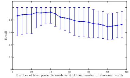
Fig. 12. Recall results of the proposed anomaly localization procedure.
the most accurate results. Although, the minimum area under the precision-recall curve for the EM learning algorithm is less than the area under the corresponding curve for the VB algorithm. It means that the variance among the individual curves for the EM learning algorithm is larger in comparison with the VB learning algorithm.
The variance of the precision-recall curves for both VB and GS learning algorithms is relatively small. However, the VB learning algorithm has the curves higher than the curves obtained by the GS learning algorithm. It can be con-firmed by examination of the best and worst precision-recall curves (Fig. 10) and the mean values of the area under curves (Fig. 8 and Table II).
We also present the results of classification accuracy, i.e., the fraction of the correctly classified documents, for anomaly detection, which can be achieved with some fixed threshold. The best classification accuracy for the EM learning algorithm in both data sets can be found in Table III.
4) Anomaly Localization: We apply the proposed method
[image:12.612.328.541.368.496.2]the EM learning algorithm with the prior type H +1 on both data sets in Fig. 11. The red rectangle is manually set to locate the abnormal events within the frame, the arrows correspond to the visual words with the smallest marginal likelihood computed by the algorithm. It can be seen that the abnormal events correctly localized by the proposed method. For quantitative evaluation, we analyze 10 abnormal events (5 from each data set). For each clip, for a given
number Ntop of the least probable words, we measure the
recall: recall=(TP/Nan), whereNanis the maximum possible
number of abnormal words among Ntop, i.e., Nan = Ntop if
Ntop≤ Ntotal an, whereNtotal anis the total number of abnormal
words, and Nan=Ntotal an if Ntop>Ntotal an. Fig. 12 presents
the mean results for all events. One can notice, for exam-ple, that when the localization procedure can possibly detect 45% of the total number of abnormal words, it correctly finds
≈90% of them.
VII. CONCLUSION
This paper presents two learning algorithms for the dynamic topic model for behavior analysis in video: the EM algorithm is developed for the MAP estimates of the model parameters and a VB inference algorithm is developed for calculating the posterior distributions of them. A detailed comparison of these proposed learning algorithms with the GS-based algorithm developed in [21] is presented. The differences and the similar-ities of the theoretical aspects for all three learning algorithms are well emphasized. The empirical comparison is performed for abnormal behavior detection using two unlabeled real video data sets. Both proposed learning algorithms demonstrate more accurate results than the algorithm proposed in [21] in terms of anomaly detection performance.
The EM learning algorithm demonstrates the best results in terms of the mean values of the performance measure, obtained by the independent runs of the algorithm with different random initializations. Although it is noticed that the variance among the precision-recall curves of the individual runs is relatively high, the VB learning algorithm shows the smaller variance among the precision-recall curves than the EM algorithm. The results show that the VB algorithm answers are more robust to different initialization values. However, it is shown that the results of the algorithm are significantly influenced by the choice of the hyperparameters. The hyperparameters require additional tuning before the algorithm can be applied to data. Note that the results of the EM learning algorithm only slightly depend on the choice of the hyperparameters’ settings. More-over, the hyperparameters can be even set in such a way as the EM algorithm is applied to obtain the maximum likelihood estimates instead of the MAP ones. Both the proposed learning algorithms—EM and VB—provide more accurate results in comparison to the GS-based algorithm.
We also demonstrate that consideration of marginal like-lihoods of visual words rather than visual documents can provide satisfactory results about locations of anomalies within a frame. To our best knowledge, the proposed localization procedure is the first general approach in probabilistic topic modeling that requires only the presence of spatial information encoded in visual words.
APPENDIXA
EM ALGORITHMDERIVATIONS
This appendix presents the details of the proposed EM learning algorithm derivation. The objective function in the
EM algorithm is
Q( , old)+logp( |β,α,η,γ)
=
y1:Ttr
z1:Ttr
(p(y1:Ttr,z1:Ttr|x1:Ttr,
Old)
×logp(x1:Ttr,y1:Ttr,z1:Ttr| ,α,β,γ,η))
+logp( |β,α,η,γ)
=Const+
z1∈Z
(logπz1 p(z1|x1:Ttr,
Old))
+ Ttr
t=2
zt∈Z
zt−1∈Z
(logξzt,zt−1 p(zt,zt−1|x1:Ttr,
Old))
+ Ttr
t=1
Nt
i=1
yi,t∈Y
(logφxi,t,yi,t p(yi,t|x1:Ttr,
Old))
+ Ttr
t=1
Nt
i=1
zt∈Z
yi,t∈Y
(logθyi,t,zt p(yi,t,zt|x1:Ttr,
Old))
+
z∈Z
(ηz−1)logπz+
z∈Z
z′∈Z
(γz−1)logξz,z′
+
z∈Z
y∈Y
(αy−1)logθy,z+
y∈Y
x∈X
(βx−1)logφx,y.
(44) On the M-step, the function (44) is maximized
with respect to the parameters with fixed
values for p(z1|x1:Ttr,
Old), p(z
t,zt−1|x1:Ttr,
Old),
p(yi,t|x1:Ttr,
Old), p(y
i,t,zt|x1:Ttr,
Old). The optimization
problem can be solved separately for each parameter, which leads to (6)–(8).
On the E-step, for the efficient implementation, the forward– backward steps are developed for the auxiliary variablesα´z(t) andβ´z(t)
´
αz(t)def= p(x1, . . . ,xt,zt =z| Old)
=
z1:t−1
πzOld1
⎡ ⎣
t−1
´
t=2
ξzOld´t,z´t−1
⎤ ⎦
⎡ ⎣
t−1
´
t=1
Nt´
i=1
y∈Y φxOldi,t´,yθ
Old
y,zt´
⎤ ⎦
×ξzOldt=k,zt−1 Nt
i=1
y∈Y
φxOldi,t,yθOldy,zt=z. (45)
Reorganization of the terms in (45) leads to the recursive expressions (10).
Similarly forβ´z(t)
´
βk(t)def= p(xt+1, . . . ,xTtr|zt =z,
Old)
=
zt+1:Ttr ξzOldt+1,z
t=z
⎡ ⎣
Ttr
´
t=t+2
ξzOld ´ t,zt−´ 1
⎤ ⎦ × Ttr ´
t=t+1
Nt´
i=1
y∈Y
φxOld i,t´,yθ
Old
y,zt´. (46)
The recursive formula (11) is obtained by interchanging the terms in (46).
The required posterior of the hidden variables
terms p(z1|x1:Ttr,
Old), p(z
t,zt−1|x1:Ttr,