Rochester Institute of Technology
RIT Scholar Works
Theses
Thesis/Dissertation Collections
7-2017
Comparing Economic, Environmental, and Social
Effects of Central Air Conditioner Size and
Thermostat Schedule Interactions
Briana Elizabeth Amoroso
Follow this and additional works at:
http://scholarworks.rit.edu/theses
This Thesis is brought to you for free and open access by the Thesis/Dissertation Collections at RIT Scholar Works. It has been accepted for inclusion in Theses by an authorized administrator of RIT Scholar Works. For more information, please [email protected].
Recommended Citation
DEPARTMENT OF INDUSTRIAL AND SYSTEMS ENGINEERING KATE GLEASON COLLEGE OF ENGINEERING
ROCHESTER INSTITUTE OF TECHNOLOGY ROCHESTER, NEW YORK
CERTIFICATE OF APPROVAL
M.S. DEGREE THESIS
The M.S. Degree Thesis of Briana Elizabeth Amoroso has been examined and approved by the thesis committee as satisfactory for
the thesis requirement for the Master of Science degree
Approved By:
Dr. Katie McConky, Co-Advisor – Industrial & Systems Engineering Department
Dr. Eric Hittinger, Co-Advisor – Public Policy Department
Dr. Brian Thorn – Industrial & Systems Engineering Department
COMPARING ECONOMIC, ENVIRONMENTAL, AND SOCIAL EFFECTS OF CENTRAL AIR CONDITIONER SIZE AND THERMOSTAT SCHEDULE INTERACTIONS
A Thesis
Submitted in partial fulfillment of the requirements for the degree of Master of Science in Sustainable Engineering
in the
Department of Industrial and System Engineering Kate Gleason College of Engineering
by
Briana Elizabeth Amoroso
ABSTRACT
Selecting the capacity of a central air conditioning (AC) system is based on a long list of structural factors within a home, but is normally chosen without considering effects on stakeholders outside of the home. Energy use by residential air conditioners is relevant to consumers as an expense, but also to utilities as a contributor to peak demand and to society by the resultant carbon dioxide and other emissions. In this article, we investigate how size and operational patterns of central residential air conditioners interact with stakeholder benefits and costs. The case study analyzes energy use for systems sized from 3.0-5.5 tons in single family homes in Phoenix, Arizona and quantifies the costs and benefits to homeowners, electric utilities, and society. For homeowners, larger units are preferred due to lower energy
consumption, leading to lower net costs, and the ability to cool the house quickly. However, under the same conditions, a smaller AC system can provide double the potential profit to the utility from reduced generation and peak load costs. As a result of lower energy consumption, larger units have lower environmental externality costs from carbon and criteria pollutant emissions. However, a social perspective that considers homeowner, utility and externality costs together results in an overall preference for smaller units with setback schedules, driven by the value of peak demand reduction.
ACKNOWLEDGMENTS
This document has taken a village to write and edit, ideate and solidify, cry and leap for joy.
My most humble thanks to my advisors who helped me through this extensive process. Dr. McConky kept me from losing my sanity when it was most important. I appreciate her attention to detail, expansive systems thinking, and the selfless time she spent helping me. Dr. Hittinger provided the basis of this work and a look into a new world I knew little about, but have come to fully embrace as an exciting new career. Dr. Thorn simply kept me laughing, which is essential for this and all journeys. Many other professors
kept me on track and provided invaluable insights along the way.
I’m indebted to my friends at RIT and especially those in the Sustainable Engineering program and the Industrial and Systems Department for staying late, going in early, sharing meals, conducting coding
sessions, and enjoying the occasional walk. Thanks especially to Kathleen, Teija, Manu, and Glenn!
To my family and friends, thank you for lending your ears and editing skills and helping me see it through. You are the best!
Sometimes in the early morning on my way to class, I walked past the sign for Kate Gleason College of Engineering. I could hardly believe I had the honor to enter these halls, after dreaming of becoming an engineer for many years. Addressing the KGCOE students on stage at graduation was the first time I truly
Table of Contents
1. Introduction ... 1
2. Problem Statement & Purpose ... 1
3. Background ... 3
3.1 The State of Central AC in the Home... 3
3.1.1 Energy Consumption ... 3
3.1.2 Current State of AC Sizing ... 3
3.1.3 Role of Thermostats and AC system Efficiency Characteristics ... 5
3.2 Peak Power and Peak Power Management... 6
3.2.1 Peak Power ... 7
3.2.2 Load Shedding & Load Shifting ... 9
3.2.3 Demand Response ... 9
3.2.4 Central AC Peak Power Example: Oklahoma Gas & Electric ... 10
3.3 Significance ... 10
4. Literature Review ... 11
4.1 Air Conditioner Sizing ... 11
4.2 Thermostat Schedules... 12
4.2.1 Human Behavior ... 12
4.2.2 Smart Technologies ... 13
4.3 Economic Costs ... 13
4.4 Environmental and Social Costs ... 14
5. Methodology ... 15
5.1 Simulation & Data Collection ... 16
5.1.1 EnergyPlus ... 16
5.1.2 AC system ... 16
5.1.3 Thermostat Schedule ... 17
5.2 Location, House Design and Construction ... 18
5.3 Economic Analyses ... 20
5.3.1 Electricity Cost To The Consumer ... 21
5.3.2 Net Present Cost ... 21
5.3.3 Peak Load Costs ... 22
5.3.4 Cost of Generation ... 23
5.4 Environmental Analysis ... 23
5.4.1 Marginal Emissions Factors ... 23
5.5 Social Cost Analysis ... 24
5.5.1 The APEEP Model ... 24
5.5.2 Net Benefit for Society ... 24
6. Results ... 26
6.1 Outcomes for Homeowners ... 26
6.1.1 Direct Energy Consumption & Cost... 26
6.1.2 Unmet Loads ... 27
6.1.3 Net Present Cost ... 29
6.2 Outcomes for the Utilities ... 30
6.2.1 Generation Cost ... 30
6.2.2 Peak Loads ... 31
6.3 Emissions and Social Outcomes ... 32
6.3.1 Emissions ... 32
6.3.2 Total Social Cost ... 40
7. Discussion ... 42
7.1 Impacts of Individual Output Metrics ... 42
7.1.1 Energy Consumption and Electricity Cost to the Homeowner ... 42
7.1.2 Unmet Loads ... 44
7.1.3 Net Present Cost ... 52
7.1.4 Cost of Generation ... 53
7.1.5 Peak Load Costs ... 54
7.1.6 Marginal Emissions Factors ... 55
7.1.7 Social Costs ... 56
7.2 Impacts to Stakeholders ... 57
7.2.1 Homeowners ... 57
7.2.2 Utilities ... 59
7.2.3 Society ... 63
8. Conclusions and Future Work ... 66
List of Figures
Figure 1: A 4-ton AC system, indoor temperature versus cooling set point over one summer day ... 5
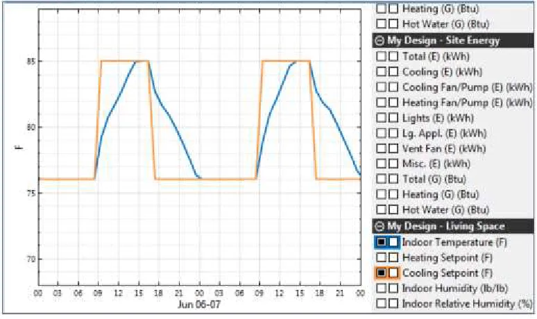
Figure 2: A 2-ton AC system, indoor temperature versus cooling set point over one summer day ... 5
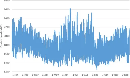
Figure 3: 2015 Hourly Load for Western NY ... 7
Figure 4: Example of peak power over 24 hours [15] ... 8
Figure 5: Using large (5.5 ton) and small (4.0 ton) capacity AC systems, average hourly energy consumption is shown over a typical 2-day period (June 4-5) in Phoenix, AZ. ... 9
Figure 6: NREL's TMY outdoor temperatures used in the simulation against the three set point starting temperatures ... 19
Figure 7: Capital investment cost of AC systems used to calculate economic analysis. ... 22
Figure 8: Energy consumption of each scenario ... 26
Figure 9: Direct cost of energy consumption to homeowner for one year. ... 27
Figure 10: Hours and magnitude of unmet load in the older home... 28
Figure 11: Hours and magnitude of unmet load in the newer home ... 29
Figure 12: Net present cost to the homeowner ... 30
Figure 13: Cost to local utility to generate power for one year. ... 31
Figure 14: Marginal carbon dioxide emissions for all scenarios ... 33
Figure 15: Dollar value impacts from particulate matter emissions of 2.5 microns or less ... 34
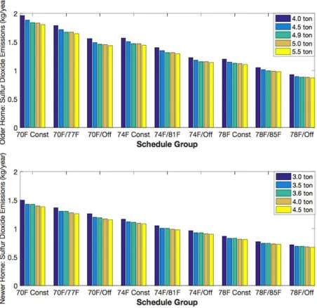
Figure 16: Marginal emissions results for sulfur dioxide ... 35
Figure 17: Impacts in dollars for yearly sulfur dioxide emissions ... 36
Figure 18: Marginal nitrogen oxides emissions for all scenarios ... 37
Figure 19: Impacts in dollars for yearly nitrogen oxides emissions ... 38
Figure 20: Social impact in dollars of ammonia emissions for all scenarios ... 39
Figure 21: Impacts in dollars of yearly VOC emissions ... 40
Figure 22: Older home: The change in overall total societal cost (TSC) components relative to the Manual J baseline for its three components: utility costs (generation and peak load costs), homeowner (initial investment cost), and emissions (social cost of emissions). ... 41
Figure 23: Newer home: The change in overall total societal cost (TSC) components for the newer home relative to the Manual J baseline for its three components: utility costs (generation and peak load costs), homeowner (initial investment cost), and emissions (social cost of emissions). ... 41
Figure 24: Comparing costs for a 5-ton & 4.5-ton system across schedules in an older home ... 44
Figure 25: Three capacities running to meet the set point in the older home for a 70°F/77°F setback schedule ... 45
Figure 26: Three capacities running to meet the set point in the older home for a 70°F/Off setback schedule. ... 45
Figure 27: The indoor temperature of the older home using a 4.9-ton system during the second week of each summer month for the 70°F/Off schedule. ... 46
Figure 28: Maximum indoor temperatures for all combinations ... 47
Figure 29: Comparing earlier setback for the 70°F/Off schedule at 4.9-tons in the older home over two summer days ... 48
Figure 30: Unmet Loads (deg-hrs/yr) and Electricity Consumption (kWh/yr) for a smart thermostat and various hours of setback for a 70°F/Off schedule in the older home, using the middle range 4.9-ton Manual J size... 50
Figure 31: The number of unmet loads as expressed in degree-hours for every $100 of net present cost, arranged by AC system capacity. Data is for both homes and the 70°F/Off schedule group that had the largest unmet loads of any schedule group. ... 53
Figure 32: Annual generation cost as a percentage of the price of electricity consumption for both house types. ... 54
Figure 34: Total Societal Cost in the older home against unmet load hours. ... 64 Figure 35:Total societal cost (bars) with unmet load hours (lines) for the newer home ... 65
List of Tables
Table 1: Energy model inputs ... 16 Table 2: Summary of simulated thermostat schedules with three schedule types and three starting set point temperatures. These nine schedules were used for each AC capacity and both new and old home
construction type over the weekday from 1 March – 30 November. ... 18 Table 3: Older Home BEopt specifications based on the modeled home from Walsh et al. ... 20 Table 4: Purchase prices used in this study. Average prices for commercially available AC systems in sizes 3.0-, 3.5-, 4.0-, 5.0-ton and interpolated prices for non-commercially available 3.6-, 4.9-, 5.5-ton AC systems. ... 22 Table 5: Peak load costs for the old home. ... 32 Table 6: Peak load costs for the new home. ... 32 Table 7: Comparing annual unmet loads and electricity consumption by switching from a 10-hour (8am-6pm) to 8-hour (8am-4pm) setback schedule in the older home using the 70°F/Off schedule. ... 48 Table 8: Results from using a smart thermostat and various setback schedules. ... 51 Table 9: The difference in net benefits of the smallest system over the largest system, for both the
electrical utility and the homeowner. ... 63 Table 10: Stakeholders and their individual priorities, which are either a output metric or part of a output metric examined in this study. The differences between each stakeholder lead to various tradeoffs
1. Introduction
The number of U.S. homes with central air conditioning (AC) grew from 68% in 1993 to 87% in 2009. These homeowners spend $11 billion on air conditioning each year [1], [2] corresponding to about 13% of their household energy consumption. In addition to economic costs, there are environmental impacts from the pollutants released due to electricity generation. The average central AC system uses 2,000 kWh annually, with consequential emissions of 3,500 pounds of carbon dioxide and 31 pounds of sulfur dioxide [3]. These and other pollutants are associated with measurable human health effects. The aggregate of homes with air conditioning also contributes significantly to electrical loads. In warmer climates such as California, 30% of the peak electricity demand during the summer months is created by air conditioning use [4]. These economic, environmental, and social effects will continue to grow, as almost 90% of newly built homes in the U.S. have central AC [2].
The size of an AC system and its thermostat schedule, i.e. its operational pattern based on user preferences, jointly affect energy consumption and consumer costs. A large capacity central AC system maintaining a constant temperature in the home has the potential to consume more energy than a smaller one since it has a higher rated power. However, the amount of energy consumed depends on its
operational pattern, which in turn is determined by its thermostat setting. Additionally, AC systems are often oversized, leading to various inefficiencies and wasted energy. The benefits of a larger AC include faster cooling whereas the benefit of a smaller unit includes lower capital cost and lower peak demand. For example, a homeowner with a smaller system that turns off the AC while away must wait longer for their living space to return to their desired temperature when they return. Although these general trends are understood, the tradeoffs between the larger and smaller capacities have not been quantified. The additional layer of homeowner’s thermostat schedule further complicates the tradeoffs. Current AC sizing guidelines do not consider these tradeoffs, nor do they consider the impacts to the major stakeholders from the three-dimensional sustainability (social, environmental, economic) point of view.
This research investigated the interaction between the capacity of a central air conditioning system, thermostat schedule and set point temperature for Phoenix, AZ. The results revealed the AC size and schedule combination that realized optimal economic, environmental and human health outcomes for three main stakeholders: the electrical utilities, society, and the residential consumer.
2. Problem Statement & Purpose
system design features and its operation settings” [5]. This research aims to close a piece of that gap. The following sections review previous research around this topic. As Solaimani et al. noted, in order to motivate energy reduction, more research exploring the role of each stakeholder is needed [6]. Expanding the selection criteria of power-hungry equipment is needed, given the context of climate change and increases in renewable energy sources that can destabilize the grid.
AC size and thermostat schedule interact in a variety of ways. For example, larger AC systems initially cost more, but enable faster temperature control with shorter duty cycles. Small air conditioners cost less upfront, but have less flexible thermostat scheduling ability because they take longer than a larger system to cool a given load. A homeowner using setbacks must set a desired temperature earlier in the day for a smaller system to reach that temperature. Smaller systems run for longer at lower power than that of a larger system because they take longer to reach a desired temperature. However, a small unit may be inefficient at cooling the house. If a smaller system is recommended for a home and the consumer will save money by using a certain thermostat schedule, what will be the associated burden placed on the transmission and distribution (T&D) utility and power generators? These smaller units consume more energy over time than larger ones since they must run for longer, meaning more electricity will need to be produced. What health costs are associated with this choice? Emissions change depending on the energy mix of the region as well as the amount of electricity consumed and the time at which it was consumed. The answer to these questions can inform decisions made by each stakeholder to reduce costs and undesired effects. For example, potential policy by way of subsidies or other incentives will be explored for the utility stakeholders.
The purpose of the research developed and presented in this thesis is to identify the tradeoffs between economic and environmental outcomes depending on an AC system’s capacity and thermostat schedule. This work explored how the combinations of various AC capacities and thermostat set points affect energy consumption from the centralized grid. In order to motivate energy reduction, more research exploring the individual role surrounding each stakeholder is needed [6]. The homeowner is the first stakeholder. The power generation utility and transmission and distribution (T&D) utility are treated as another stakeholder. The third stakeholder is society as a whole. The thesis research considered each stakeholder’s priorities to fill knowledge gaps in both economic effects and avoided emissions. Results will be in terms of factors such as human health costs, private costs, effects of peak usage, and marginal environmental emissions.
choose the AC size given thermostat scheduling preferences. Although the scenarios that save the most energy may be obvious, the lifetime costs and tradeoffs between money and comfort is not. By
understanding these interdependencies, consumer motives can be leveraged. Utilities benefit through demonstrated rebates on AC capacities that can decrease their costs and increase net revenues.
3. Background
In this section, homeowner energy demand and consumption is explored in terms of AC usage as well as the utility’s role in peak power production, management, and attempts at curtailment.
3.1
The State of Central AC in the Home
The following sections explore the role of central AC use in residential U.S. homes within the context of overall energy consumption as well as how thermostats influence consumption. Similarly, there is a discussion on how the capacity of a household’s AC system is typically determined, as this is one of the two main parameters analyzed in the research.
3.1.1 Energy Consumption
One-fifth of the US housing stock, or 11.9 million homes, were built in the 1980s [7] and have AC equipment over 20 years old. These older systems have lower efficiencies, which increases energy consumption. Even houses with AC systems that are just 10 years old could be saving as much as 20- 40% on their energy consumption by using a newer model [3]. This increase in cost does not include the impacts associated with the construction of older homes, which tend to leak conditioned air more than newer homes. To curb these inefficiencies, the Environmental Protection Agency (EPA) and Department of Energy (DOE) as well as state governments have mandatory energy standards for new homes. Energy efficiency is further impacted because only 42% of homes using AC perform regular maintenance on their equipment [2]. Electrical energy consumption from AC systems is also determined through efficiency characteristics. For example, increases in recirculation rate, supply and return duct leakage, fan power draw, and relative humidity increase the operating time of the equipment, which is the ultimate driver of electricity consumption [8].
3.1.2Current State of AC Sizing
recommend an AC capacity that will cool the home for all but 1%, or 88 hours, of the year given a location’s typical 30-year hottest temperature. This method is widely used as the national standard either alone or as a basis for a contractor’s calculations.
Before government standards became stricter, Heating Ventilation and Air Conditioning (HVAC) contractors developed their own rules-of-thumb to choose how large of a system will provide sufficient cooling to the house. Many contractors still use these self-developed guidelines [9], one reason being to avoid customer callbacks. When these practices take place, oversizing occurs most of the time [10]. Oversizing can also be due to contractors adjusting their calculations to be closer to the generic “400 square feet” rule-of-thumb that designates one ton or 12,000 Btu-hours of air conditioning capacity will
cool about 400 ft2 [9]. Further overcorrection occurs when a contractor adjusts for poor construction that does not meet building codes. ENERGY STAR notes that improperly oversized ACs are “recognized as a common industry problem” [11]. ENERGY STAR’s manual on correctly sizing ACs explains that oversized units lead to more expensive initial and lifetime costs. Systems are less frequently undersized, leading to other problems such as insufficient cooling capacity and decreased comfort. An example of how sizing affects indoor temperatures is seen in Figure 1 and Figure 2 generated using the BEopt software discussed in the Literature Review. The graphs of temperature over time show the simulated difference between a given cooling load as handled by a 4-ton AC system and a 2-ton AC system
Figure 1: A 4-ton AC system, indoor temperature versus cooling set point over one summer day
Figure 2: A 2-ton AC system, indoor temperature versus cooling set point over one summer day
3.1.3Role of Thermostats and AC system Efficiency Characteristics
[image:13.612.118.505.350.580.2]unit will cycle on and off. The length of time for which the AC runs is called its duty cycle.
With programmable thermostats, users have the option to create programs, or schedules, in which the set point will change at specified times and dates. The thermostat follows predetermined set point guidelines based on the sensed environment. In the U.S., programmable thermostat usage is split mostly by region. Of the 38% of homes that have programmable thermostats in the warmer south, 67% use their central AC every day during the summer [2]. Unfortunately, research has shown that a consumer owning a programmable thermostat does not mean that the thermostat is used correctly or even at all. Pritoni et al. used a crowd sourced online survey, asking participants to upload photos of their programmable
thermostat to prove their actions were consistent with reported behaviors. The researchers found that one-third of participants did not use the programming capacity of their thermostat. Misuse of the thermostat was prevalent. Examples included incorrect current time and date thereby nullifying the effects of the thermostat schedule, confusing the current temperature of the room for the set point temperature on the display, or accidentally placing the thermostat on “hold” when reporting that it was set to a program. A “hold” is when the user overrides the system’s programmed thermostat schedule manually. This action keeps the desired temperature at a constant degree until the user manually removes the “hold”. Consumers often don’t understand how AC technology works. One-third of participants in the study believed the myth that setting back the temperature when no one is home during warmer months uses more energy than holding at a constant lower temperature [12]. The authors ended their paper by estimating that internet-connected programmable thermostats are installed in over 4 million North American homes and that the number of misused thermostats will continue to grow, an important insight given the next topic.
More recently, smart thermostats have appeared on the market bringing more energy savings potential than their predecessors [13]. This technology allows users to switch the set point remotely from a smartphone or computer. The technology aligns the thermostat schedule more closely to the user’s habits. One type of smart thermostat called a learning thermostat, such as Google’s Nest, learns user-preferred behavior and self-corrects. Smart thermostats also attempt to optimize thermostat schedule based on external inputs of electricity price to assist the user in avoiding costs. These optimizations can be manually overridden at any time by the user. Additionally, smart thermostats assist with the problems associated with programmable thermostats by providing transparency and higher usability to increase user comprehension, these features can help the user take advantage of the benefits provided by a
programmable thermostat.
3.2
Peak Power and Peak Power Management
for western New York State over the year 2015 [14]. This data was chosen as it is more readily available than other locations. The figure shows that not only is there more load in the warmer summer months, but the peaks are higher as well. Electricity use during this time contributes to higher impacts on the
[image:15.612.89.524.214.476.2]environment and a transmission and distribution utility’s bottom line. The impact on the utility is so great that utilities use various means to avoid consumption and lower the need of a power generator utility to generate electricity during this time. The reasons for this are discussed in the following subsections. An example of a utility’s peak demand avoidance using demand response (DR) programs is also detailed.
Figure 3: 2015 Hourly Load for Western NY
3.2.1Peak Power
demand because it makes the grid less stable and increases the chance of outages. To keep the grid stable, the electrical grid is built to have a larger capacity than necessary, leading to environmental burdens [17]. Since peak power is also more expensive to generate, those increased prices and environmental burdens are passed to the customer.
[image:16.612.150.463.261.471.2]The activity for this period is especially high during the summer months when homeowners turn on their ACs or lower their thermostat settings in anticipation of returning home. For example, in Texas two-thirds of electricity use (peak and non-peak) in the summer is from AC usage [18]. This high use creates a higher demand on the grid [15]. There are dedicated power plants, called peaker plants that are used to increase electrical generation to meet peak demand.
Figure 4: Example of peak power over 24 hours [15]
on but quickly decline in hourly energy consumption because they reach the cooling set point faster than the smaller unit. Since smaller systems are unable to cool quickly, their peak consumption period is lower but spread over more time.
Figure 5: Using large (5.5 ton) and small (4.0 ton) capacity AC systems, average hourly energy consumption is shown over a typical 2-day period (June 4-5) in Phoenix, AZ.
3.2.2Load Shedding & Load Shifting
To manage peak demand, a strategy called peak shifting or load shifting can be used. Load shifting is when the load usually needed during peak time is demanded at a different time [17]. One way to shift load from an AC during peak times is by precooling the home, simply meaning that the house is cooled ahead of peak demand. Precooling is more efficient in terms of reducing peak power demand and therefore avoids environmental impacts due to power generation infrastructure and extra energy
production [17]. Load shedding is when the load during that time is no longer demanded.
3.2.3Demand Response
3.2.4Central AC Peak Power Example: Oklahoma Gas & Electric
The SmartHours program used by the utility Oklahoma Gas & Electric (OGE) illustrates how much utilities value removing peak demand. Air conditioning units turn on at similar times throughout a given region and therefore contribute to peak power load. Due to this effect, OGE provided incentives to their customers to move their demand to hours outside of peak times. By the simple distribution and free installation of a free programmable thermostat that alerts users to changes in upcoming energy pricing, a total of 2 kW peak demand per home was avoided since the program began [22]. In 2012, a total of 70 MW peak demand was removed from the 40,000 homes in the program [23]. Aside from the
programmable thermostats, the SmartHours program experimented with smart metering, web portals for online management, and in-home displays to monitor energy consumption. OGE concluded that smart thermostats provide the most control over reduction in electricity consumption. OGE aims to defer investment in 170 MW of power plant infrastructure through such programs [24].
3.3 Significance
The results of this thesis identified the effects of the interactions between AC system size and thermostat schedule. In recent years, the method to curb residential energy has leaned toward managing energy demand at the point of consumption, such as with Demand Side Management (DSM). DSM is used by utilities to invest in reducing demand instead of investing in new infrastructure. As Palensky et al. explains, the main advantage of DSM is economic. Rather than build a new power plant or infrastructure to keep up with new demand, it is cheaper to lower the demand itself [25]. This idea is reflected in the motivation for the Oklahoma Gas & Electric free thermostat program. Palensky et al. states that the most important DSM type is Energy Efficiency, however the best option overall is the optimized combination of all categories as determined by economic incentives [25]. This research offers the beginning steps to fill this gap.
Finding ways to better control the consequences of power hungry equipment is more important than ever given the context of climate change, increases in renewable energy sources that destabilize the grid, and the trend in the reduction of coal mining [26], a common fuel for baseline energy production. Additionally, the International Energy Agency [27] has demonstrated that overall peak load will continue to increase over the next 35 years. Due to the challenges associated with generating and consuming peak power, efforts should be made to reduce and manage its generation and consumption. An improved understanding of the changes in greenhouse gas emissions from peak power reduction is important to the continued commitment to stricter emissions standards [28].
make more informed decisions, positively impacting their wallet and environment. Socially focused policy makers and profit driven utility companies alike can evaluate tradeoffs to find incentives for consumers to reduce energy use, spare T&D losses, lower pollution emission rates, and save money.
4. Literature Review
This section explores existing literature surrounding the two main parameters to be analyzed, AC size and thermostat schedule. The human health, economic, and environmental aspects of using power from the central electrical grid is also discussed.
4.1
Air Conditioner Sizing
The American Society of Heating, Refrigerating, and Air-Conditioning Engineers (ASHRAE) 2013 Handbook of Fundamentals explains the major methods of AC sizing. The previously mentioned,
Manual J of ACCA (8th edition) standard is widely used in the U.S. The calculations for the Manual J is based on experiments performed at the University of Illinois in the 1950s. Other methods include older versions of the ASHRAE Fundamentals Handbook between 1985 and 2001 that were the result of research performed in 1984. The research model included outdoor temperature swings, an important consideration for thermostat schedules. The final method noted in the Handbook is the Canada F280 method, which is based on the same research of the older ASHRAE versions [29].
An HVAC sizing strategy guideline from the DOE [9] does not consider how the operational pattern may affect sizing. The guide explains how oversizing for the house can be detrimental for the
system and the user. For example, the guide offers the analogy of a car’s improved gas mileage on the highway to explain that the longer an AC system runs, the better. Short duty cycles stress AC equipment and decrease both efficiency and effectiveness. According to the guidelines, the most efficient and optimized mode for the AC equipment is to run for longer periods of time. Shorter cycles disallow for proper dehumidification because the unit is not running long enough for the coil to obtain the necessary temperature.
Electric utilities occasionally release recommendations for HVAC contractors to avoid this problem [31], but complaints of oversizing are still pervasive throughout discussions of AC sizing. Complaints are so common that the major influencers of energy efficiency in the U.S. have released their own literature both to raise awareness for consumers and to dissuade contractors from making poor calculations. Some of these institutions include the National Renewable Energy Lab (NREL) [9], ENERGY STAR [11], and ASHRAE [10].
4.2
Thermostat Schedules
Aside from AC size, the other major parameter analyzed in this study is the operational pattern of a programmable thermostat. According to the DOE, a seven to 10°F setback (or increase) of temperature for at least eight hours a day can save about 10% on home cooling and heating costs [32]. The following sections describe how thermostat usage is affected by a user’s behavioral patterns and how the emerging field of smart technology is important to reducing residential energy consumption.
4.2.1 Human Behavior
4.2.2 Smart Technologies
Smart technology is a new way to control thermostat schedules. Manufacturers promise larger energy reductions by more precise control over the runtime of an AC system. A smart home technology literature review points out that the technology is “not commercially exploited [which] makes it clear that there must be plenty of strategic, organizational and financial issues that require further attention” [27]. Exploring the issues that surround the smart thermostat more in-depth is important to motivate the customer stakeholder to see reduced energy usage across the grid. There are many papers that investigate how to extend the smart home with individual appliance use [35] or integrate the whole smart home system, such as in [38] and [39]. Studies often explore these network designs [38]–[40] while others form a schedule to avoid peak demand [41], although do not consider AC size. There is clearly a lack of research informing AC size and smart scheduling interactions.
4.3 Economic Costs
This thesis research considers costs associated with the generation of peak power. Peak load literature often explores user-response to peak demand pricing changes such as [20] and [42]. Using a simulation of 900 homes, Cole et al. found a new peak is not created when a community responds to changing electricity prices through load shifting [43]. They explored various strategies to reduce peak demand [43]. End-users respond to price changes as a motivator to reduce consumption during certain hours of the day. Enabling technologies, or technologies that help the consumer avoid peak prices such as a smart thermostat, have substantial opportunity to further enhance potential savings. For example, Faruqui et al. found that when enabling technologies respond to Critical Peak Pricing, whole house energy consumption dropped by 27-44% [44]. The potential savings from reducing energy use through timing is significant. As Newsham et al. describe it, the potential value to the customer is clear [20]. Reducing energy consumption 2-5% during peak hours can reduce the price charged to the customer by 50% or more. That reduction can become $3 billion in annual savings across the grid if the top 1% of peak consumption is reduced by only 5% [45]. Electric utilities are willing to pay for reduction in peak power through demand response programs, such as “Power Manager” from Duke Energy, which pays $32/year to customers to allow the utility to control their AC systems for a predetermined number of times. ConEdison promises commercial customers up to $18,000 per year for reducing energy usage during peak times in their demand response program [46]. According to electrical utility software
company Opower, utilities spent $580 million in 2013 on demand response programming in an attempt to avoid peak loads, which is worth $94/year for one kilowatt of peak power on national average [47].
modeled [48]. Rhodes et al. examined energy audit data in Austin, Texas and showed that 31% of the 5,000 reviewed houses had oversized AC systems, leading to excess peak power load of 41 MW. Rhodes et al. then retrofitted the ACs to the correct size and implemented other efficiency improvements as suggested by the ENERGY STAR Home Performance program from the DOE and EPA. The authors quantified the amount of excess load that could be removed by comparing that year’s data to historical peak power data. The resulting peak power demand savings were expressed as a benefit to the utility by equating the total potential load removal to the generating capacities of locally operating power plants [49]. The benefit of peak removal is also examined in this study, although the savings are in terms of dollars per year and consider an AC’s peak power over a year, reflecting overall peak demand costs to the utility on a magnified scale.
Electrical utilities, especially the T&D companies, gain value from reduced peak. The U.S. average of T&D losses is 6% [50]. Load shifting from peak to non-peak would reduce T&D losses from centralized power generation because losses are proportional to the square of current flow [51]. Nourai et al. found economic benefits from reducing T&D loads during peak hours [51]. Using battery storage to shift load from peak to off-peak, they calculated a net present value of a few hundred dollars over several hours due to the reduction in T&D losses. The authors also found that reducing load across multiple sites realizes higher T&D efficiencies than if reduced in only a few places, further motivating T&D companies to promote peak load reduction.
4.4
Environmental and Social Costs
Erol-Kantarci et al. explored emissions reductions by moving appliance use to off peak times [52]. Peaker plants run on fossil fuels that generate greenhouse gas emissions. Consumers can lower these emissions by improving energy management. Therefore, the study shows that lower electricity
consumption during peak hours not only lowers electricity bills, but also lowers carbon dioxide equivalent (CO2eq) emissions of a household. However, in the study, air conditioning was not part of the simulated appliances.
One method to determine social costs associated with atmospheric pollution is called the Air Pollution Emission Experiments and Policy analysis (APEEP) model. Social costs can be measured in
across different scenarios and to compare the economic costs against the social costs. The model uses
county-specific data in the units of dollars per ton of the following individual pollutants: PM2.5, SO2 (Sulfur Dioxide), Volatile Organic Compounds (VOCs), NOx (Nitrogen Oxides), and NH3 (Ammonia).
The damages included in the dollar value are the “adverse effects on human health, reduced yields of agricultural crops and timber, reductions in visibility, enhanced depreciation of man-made materials, and damages due to lost recreation services” [55]. APEEP has been used in various studies including one that considers electrical grid emissions [56].
According to the EPA, the smaller the particle size, the greater the potential damage. This is because smaller particles can not only enter a person’s lungs, but also their bloodstream. Potential health effects include asthma, heart attacks, premature death and increased respiratory symptoms. Haze and acidification of local ecosystems is another effect of small particulate matter as well as material or aesthetic damage to surrounding environments [57]. Common health effects from VOC exposure range from fatigue and dizziness to more extreme effects such as damage to the liver, kidney and central nervous system, and are also suspected of causing cancer in humans [58]. At less than a dollar per year, VOCs and ammonia both have a minimal impact whereas sulfur dioxide and nitrogen oxides make up most of the social costs.
The total kilograms of three pollutants resulting from the electricity generation of each scenario are calculated in this thesis. The first of these is carbon dioxide. Carbon dioxide is released from the burning of fossil fuels and is globally monitored as a pollutant due to its known potential to retain heat in our atmosphere beyond levels that would otherwise naturally exist. This trait is called global warming potential. In the U.S., carbon emissions make up 80% of all such greenhouse gas (GHG) emissions due to human activity, such as generating electricity to run air conditioning. As of 2014, electricity generation is the largest source of carbon dioxide emission in the United States and accounts for 30% of all GHG emissions [59]. The second pollutant considered is sulfur dioxide. The EPA describes the health effects of atmospheric sulfur dioxide as a stressor or even a cause of respiratory diseases. It can also contribute to “increased hospital admission and premature death” by complicating existing heart disease [60]. Lastly
are nitrogen oxides. Together nitric oxide (NO) and nitrogen dioxide (NO2) are nitrogen oxides commonly referred to as (NOx). Exposure to NO2 can worsen asthma as well as inflame the airway.
Ammonia reacts with NOx in the atmosphere to create small particles that the human body is more susceptible to absorbing deep into the lungs [61].
5. Methodology
the 90 simulations and associated analyses show economic costs to the homeowners and utilities, energy use, pollution emissions and social costs for each AC-thermostat schedule combination. Together, the three types of analyses create a triple bottom line sustainability analysis.
5.1
Simulation & Data Collection
This section overviews the energy modeling software and details the major inputs examined during the research. The five major simulation inputs are shown in Table 1. The two inputs detailed here are the air conditioning system to be observed and the thermostat schedules they will be matched against.
Table 1: Energy model inputs
Constant Location, weather data
Variable AC system size, thermostat schedule, age of house construction
5.1.1EnergyPlus
EnergyPlus is a building energy simulation software funded by the U.S. Department of Energy Building Technologies Office [62]. NREL’s graphical user interface to EnergyPlus is BEopt version 2.6 and was used for the simulations. BEopt was used in residential energy usage studies [45], [52], and [53].
Sousa [65] recognizes that EnergyPlus is an “integrated solution” that contributes to precise space-temperature predictions, an important step to understanding and modeling accurate system sizing. EnergyPlus is used globally and accepted by researchers as a valid tool to analyze building energy consumption and potential alternatives to promote energy reduction. Heat transfers are determined using algorithms that consider building physics. EnergyPlus has been updated twice a year since debuting in 2001 [66]. The Energy Plus software is categorized as an engineering method bottom-up technique. BEopt’s many inputs, such as climate data, temperatures, and AC system characteristics makes this technique a strong choice to model new technologies [67].
5.1.2AC system
EnergyPlus allows users to model using time step simulations for HVAC systems. This detail was necessary for this research and results were displayed in singular kilowatt-hours for the entire 8,760 hours of a year. EnergyPlus comes preloaded with HVAC systems that can be altered by individual
components. Creating a new HVAC system is also possible using an independent data set for efficiency ratings, number of speeds, capacity ratio, condenser type, fan speed ratio, rated and installed supply fan power, etc.
The modeled AC capacities ranged from the BEopt Manual J calculation for the home described in the next section, to larger systems often chosen by contractors as well as smaller capacities for comparison. The calculated Manual J value in EnergyPlus does not round to the nearest half-ton when performing its analyses. Therefore, the resulting Manual J sizes are in between commercially available sizes. Five sizes total were modeled for each thermostat schedule. The sizes included the Manual J size itself and the four choices available to an AC installation contractor: the two sizes larger than and the two sizes below the Manual J value, in increments of commercially available 0.5-tons. If a residence requires beyond a 5.0-ton capacity, common practice is to have two smaller sized units. In this study, the older construction type home, described in Section 5.2, had a Manual J value of 4.9-tons. For consistency, 5.0- and 5.5-ton units were used for the two sizes beyond the Manual J 4.9-ton value.
5.1.3Thermostat Schedule
The cooling schedules used in the simulations are detailed in Table 2. The three starting temperatures for these schedules were chosen based on industry standards and DOE recommendations. The 2013 ASHRAE Fundamentals Handbook suggests indoor temperature designs use 75.2°F as the dry bulb temperature with a maximum 50-65% relative humidity. The ASHRAE Standard 55-2013, Thermal Environmental Conditions for Human Occupancy, suggests a comfortable thermal range is between approximately 67°F and 82°F. ACCA’s Manual J uses 75°F as the desired indoor temperature for their design calculations. ENERGY STAR suggests all cooling set points are 78°F or more during occupancy [32]. To account for variance of human comfort, data from the 2009 US EIA Residential Energy
Consumption Survey (RECS) Table HC7.11 were used to choose three starting set point temperatures of 70°F, 74°F and 78°F.
temperature. A summary of these schedules is found in Table 2. A total of three schedule types (Constant, Plus Seven, Off) were modeled for each of the three starting temperatures (70°F, 74°F and 78°F). Those nine scheduling scenarios were modeled for each AC capacity described in the previous section, resulting in 45 combinations for a single home, or 90 scenarios total for the two construction types.
Table 2: Summary of simulated thermostat schedules with three schedule types and three starting set point temperatures. These nine schedules were used for each AC capacity and both new and old home construction type over the weekday from 1 March – 30 November.
Starting Set Point Temperature (set point/setback)
Schedule Type (setback period) 70°F 74°F 78°F
“Constant” (NA) 70°F/70°F 74°F/74°F 78°F/78°F
“Plus Seven” (8am-6pm) 70°F/77°F 74°F/81°F 78°F/85°F
“Off” (8am-6pm) 70°F/Off 74°F/Off 78°F/Off
5.2
Location, House Design and Construction
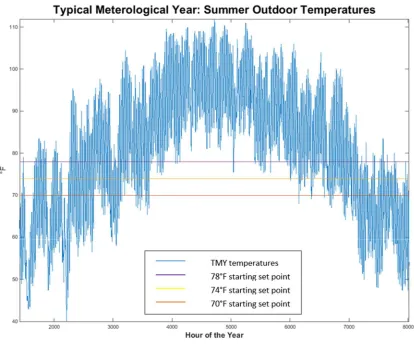
Figure 6: NREL's TMY outdoor temperatures used in the simulation against the three set point starting temperatures
The city of Phoenix’s Planning and Development Department tends to adopt national and international standards and not create other measures [60]. Therefore, the house design specification was based on local average residential units and DOE recommended values. Two overall cases will be considered to represent both new construction since 2010 and older construction that make up houses from 1980 – 2009, about 1.2 million homes in Arizona (Arizona - Table HC2.11 Structural and
Geographic Characteristics of Homes in West Region, Divisions, and States, 2009) [70]. For houses built since 2010, Building America’s B10 benchmark design, which includes 2009 IECC housing codes, was used to inform new construction. The necessary R-values for insulation and other characteristics of the B10 Benchmark is an option within the BEopt software for new construction and therefore
straightforward to model.
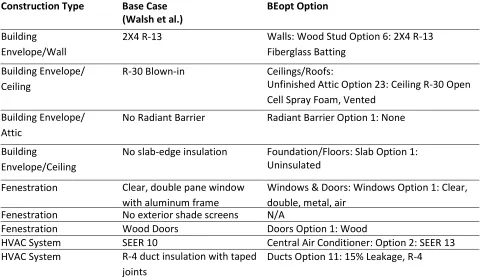
al. scenario that needed to be defined within BEopt to represent an older home. BEopt’s retrofit options informed those other characteristics as follows. Air leakage of 10 ACH50, or ten air changes per hour at a pressure difference of 50 Pascals, is considered “typical” by research cited within BEopt. Duct leakage is a significant contributor to the building envelope. The standard 15% leakage with R-4 insulation was used in this research. The refrigerator type was chosen to have the freezer on top and an Efficiency Factor of 15.9, a value between 17.6 from the B10 Case and closer to the least efficient retrofit option of 14.1. For both cases, the DOE Housing Simulations Protocols set the standard operating conditions of the house such as refrigeration, lighting, manual ventilation (such as opening windows).
Table 3: Older Home BEopt specifications based on the modeled home from Walsh et al.
Construction Type Base Case
(Walsh et al.) BEopt Option
Building Envelope/Wall
2X4 R-13 Walls: Wood Stud Option 6: 2X4 R-13
Fiberglass Batting Building Envelope/
Ceiling
R-30 Blown-in Ceilings/Roofs:
Unfinished Attic Option 23: Ceiling R-30 Open Cell Spray Foam, Vented
Building Envelope/ Attic
No Radiant Barrier Radiant Barrier Option 1: None
Building
Envelope/Ceiling
No slab-edge insulation Foundation/Floors: Slab Option 1:
Uninsulated
Fenestration Clear, double pane window
with aluminum frame
Windows & Doors: Windows Option 1: Clear, double, metal, air
Fenestration No exterior shade screens N/A
Fenestration Wood Doors Doors Option 1: Wood
HVAC System SEER 10 Central Air Conditioner: Option 2: SEER 13
HVAC System R-4 duct insulation with taped
joints
Ducts Option 11: 15% Leakage, R-4
The size of the modeled house was 2,100 square feet. US census data shows that of new construction in 2010 in the western region, most homes were in the 1,800-2,400 square foot range, with an average of 2,100 square feet [72]. Two-car garages have been common in the western US since the 1970s and therefore the generic standard sized 22’ X 22’ garage was included in the model [72]. All of the preset BEopt 2.6 settings for the building structure were kept unless otherwise discussed.
5.3
Economic Analyses
basic cost of running the system in the home, the net present cost, costs of energy generation by the power generator utility, and peak load costs to the T&D utility.
5.3.1Electricity Cost To The Consumer
The price of electricity used for this study was collected from Open Energy Information [73], an online open database populated by data from the Energy Information Agency (EIA) and was the average of the total revenue and sales of the T&D utility in the area. The EIA average rate for residential
customers in the 85041 zip code for Phoenix, AZ is 10.9 cents/kWh [74]. The pricing will remain constant throughout the entire year period of analysis to allow for comparisons with other schemes.
5.3.2Net Present Cost
The cost of owning and using the AC system to the homeowner was determined using the Net Present Cost equation for a uniform series, since there are fixed annual payments for a fixed number of periods. In Equation 1, Io was the initial investment, c was the annual cost of purchasing electricity, N was the average lifespan of the unit as given by BEopt as 16 years, and i was the discount rate set to 5%.
= + (( )) (1)
Figure 7: Capital investment cost of AC systems used to calculate economic analysis.
Table 4: Purchase prices used in this study. Average prices for commercially available AC systems in sizes 3.0-, 3.5-, 4.0-, 5.0-ton and interpolated prices for non-commercially available 3.6-, 4.9-, 5.5-ton AC systems.
3.0-ton 3.5-ton 3.6-ton 4.0-ton 4.5-ton 4.9-ton 5.0-ton 5.5-ton
$946.70 $1,052.96 $1,073.50 $1,155.67 $1,270.99 $1,363.24 $1,386.30 $1,441.14
5.3.3Peak Load Costs
The costs of meeting peak demand include the maintenance of generation, transmission, and distribution resources that are rarely (or perhaps never) used. These “costs” may better be thought of as unrealized savings that occur if peak demand can be reduced through other means, such as home energy efficiency initiatives. An average monthly demand charge for residential customers in the Arizona Public Service Electric Company of $11.40/kW is used to calculate the annual peak load cost as seen in Equation (2) [76].
= ∗ 11.40 (2)
5.3.4Cost of Generation
The generation cost (GC) metric was included because the consumer demand of energy
influences the cost of generation, which can vary drastically with time. If demand is shifted to periods of lower generation cost, both consumers and utilities benefit. The hourly wholesale energy pricing of the Arizona-New Mexico region was used to determine an annual electricity production cost as specified in Equation (3) where kwht is the electricity consumed during hour t of the simulation, and GCt is the generation cost at time t. This generation cost was calculated using the data set provided by Hittinger et al., as collected from the southeastern border of the California Independent Systems Operator [77]. This cost was calculated for each of the 90 combinations. The results provide insight into potential subsidies to decrease generation costs.
= ℎ ∗ (3)
5.4
Environmental Analysis
Two environmental analyses were performed. The first calculated the resulting pollutants emitted by using electricity from the grid. The other analysis determined the residential in-home impact of the amount of time an AC system did not reach the desired set point.
5.4.1Marginal Emissions Factors
Avoided pollution due to electricity generation will be measured by using standardized marginal emissions factors (MEFs) calculated in [78]. As previously explained, as demand increases more
generators turn on to feed the grid to meet the demand. An MEF describes how much NOx, SO2, CO2 emissions are released per unit of power as categorized by the latest generator added to the grid. For example, if the number of kWh avoided can be aggregated per each hour, then the specific MEF that matches the demand that hour can be applied. This method was used in a study showing that battery storage generally increases emissions [70]. Each state generates their electricity through varying methods at different magnitudes, which in turn affects the amount of generated emissions. The energy mix of New York state is based on mostly nuclear and hydroelectric dams, which generate fewer carbon emissions
than a more fossil fuel heavy mix. In 2013 as a result of energy generation, New York emitted 8.1 metric tons of CO2 per person, whereas Arizona had almost double that at 14.1 metric tons of CO2 per person
[79]. As of August 2015, Arizona had a mix of mostly natural gas-fired, coal-fired, and nuclear electricity generation. A less significant 1,000 GWh out of the total 12,544 GWh production was from hydroelectric and other renewables [80]. Another example of how pollutants differ across states is in the carbon
only 44.9 kg CO2 per million Btu [79].
5.4.2Unmet Loads
A metric describing unmet loads is detailed in Equation (4). In Equation (4), UHt captures the hours when the cooling load is not met, specifically UHt is equal to 1 for any time period when the indoor temperature I is greater than the desired set point a (S) with an industry standard one degree tolerance [81]. The magnitude of the unmet loads at time t, UHt, is the total observed temperature difference between the desired indoor temperature and the set point at any period t. Finally, the total unmet cooling load (UCL) is calculated in DegHrs, and is the sum of all UHt in hours across the simulation time frame. BEopt is hardcoded to only consider AC cooling between March 1st and November 30th, all 6,600 hours. Therefore, all mention of annual metrics is defined by only these nine months of AC operation.
= 1 > + 1 0 ℎ
| | = − ( + 1) = 1
0 ℎ 6,600 ℎ
= | |
(4)
5.5
Social Cost Analysis
This section first explains the APEEP model that translates pollution emissions to a price associated with its impacts on humans interacting with their environment. Secondly, the inputs used to determine optimization of the AC size and schedule combinations across society are detailed.
5.5.1 TheAPEEP Model
In order to use the correct energy mix for Phoenix and county level information, the Federal Information Processing Standard (FIPS) code for Phoenix (04-013), provided by the US Census Bureau [82], was cross-referenced with the FIPS code entries in the APEEP data available on the website of the creator of APEEP, Nick Muller [54]. The most recently available marginal prices for 2008 for the five pollutants were used and were in dollars of social cost from the year 2000 per short ton for each pollutant. These prices were multiplied by the amount of each pollutant generated in each AC combination scenario. As only state-wide rates were available, the rates for pollution emissions were calculated by finding the total emissions in tons of each pollutant due to fuel combustion for electricity generation in Arizona in 2008 from the National Emissions Inventory [83] and the total electricity generated in 2008 in Arizona from the EIA in 2008. The data was found in the electricity Data Browser under net generation for electric utility only [84].
5.5.2 Net Benefit for Society
( ) = + + + (5)
Total Societal Cost is defined as the summation of the initial investment of the AC system
(installation and purchase cost) to the homeowner (Io), the social cost of the marginal emissions results for carbon dioxide and the five APEEP social costs results (EMC), and finally, the costs of both peak load (P) and generation to the utility (GC). Generation cost was included because as homeowners determine the demand of energy, that demand influences the cost of generation. If the cost of generation decreases, so will the price of electricity and both stakeholders benefit. A similar effect occurs for peak load costs. Environmental emissions can affect the entire local population and the initial costs to the homeowner to have AC equipment matter because the sizes of the systems affect energy demand, which again can put more costs back onto both the homeowner and utilities. The costs for all 90 scenarios were evaluated and the lowest cost scenario is considered the best one for society.
For consistency, the initial net present cost was annualized using the capital recovery factor, where is annualized cost and is the initial investment, is the 16-year lifespan and was 0.05% as seen in Equation 6.
= (1 + )
(1 + ) − 1 (6)
In order to monetize the carbon dioxide results, the EPA’s social cost of carbon for the latest year of 2015 was $11 per metric ton at a 5% discount rate in year 2007 dollars [85]. The Consumer Price Index (CPI) was used so that the results would be in dollars for the year 2016. To change the APEEP prices from year 2000 and social cost of carbon from 2007 dollars to 2016 dollars, the following CPIs from the Bureau of Labor Statistics were used in Equation 7: 172.2 (Year 2000), 201.6 (Year 2007), and the 2016 CPI was the average of the four months available, 237.855 [86].
2000 2016
2000 = 2016 (7)
For example, the year 2000 price of Sulfur Dioxide according to the APEEP model is $21,777 per short ton. Therefore, the 2016 price would be about $30,000 per short ton or $15 per pound.
$21,777 237.855
6. Results
The Manual J calculated load for the newer construction, the 2010 Benchmark America home, was 3.6-tons. For the older home with different construction parameters, it was 4.9-tons. The outcomes of each output metric described in the methodology for all ninety possible combinations of older or newer home, AC capacity, thermostat set point, and schedule type are shown in this section. The results are organized by the entity directly impacted by each result beginning with the homeowner, then the power generators and T&D utilities, and finally society.
6.1
Outcomes for Homeowners
This section contains results that are relevant to the homeowner, such as direct energy cost and consumption. Homeowner comfort is accounted for in terms of when the system could not perform to the temperature set points imposed by the homeowner. Finally, the net present cost is presented.
6.1.1 Direct Energy Consumption & Cost
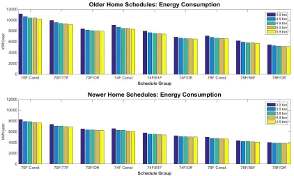
[image:34.612.78.500.402.655.2]In Figure 8, the results, like most of the graphs to follow in this section, are grouped by the schedule type and thermostat set point in ascending order. Each simulated combination had a different amount of power consumption for the one-year scenario. Less power was consumed as the set point increased as well as for the number of hours the indoor temperature was permitted to increase.
The direct cost of consumption seen in Figure 9 is directly proportional to electricity consumption in Figure 8.This direct relationship is because the energy consumption was multiplied by a constant price of 10.9 cents/kWh. Costs for the older home ranged from 24% to 28% higher than that of the newer home.
6.1.2 Unmet Loads
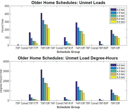
[image:35.612.78.530.166.447.2]The upper portion of Figure 10 and Figure 11 reveal the number of hours in the simulated year for which the actual indoor temperature does not meet the set point plus one degree Fahrenheit. The lower portion of Figure 10 and Figure 11 show the magnitude of that unmet load by incorporating by how many degrees it was away from the set point with an allowance of one degree above the set point. Clearly, the schedule is more influential than the AC capacity and larger capacities have fewer unmet loads. This trend is especially noticeable in how the smallest system for the older home with the 70°F/77°F schedule has the largest unmet degree-hours for that schedule group, but is still about 50% less than for the largest system in the 70°F/Off group.
Figure 11: Hours and magnitude of unmet load in the newer home
6.1.3Net Present Cost
Figure 12: Net present cost to the homeowner
6.2 Outcomes for the Utilities
Two factors that are important to the utilities are economic. First is the cost to generate power given the time of day. The second is the cost of peak power through demand charges. Both sets of results are presented in this section.
6.2.1 Generation Cost
Figure 13: Cost to local utility to generate power for one year.
6.2.2 Peak Loads
Table 5: Peak load costs for the old home.
AC Capacity (tons)
Range of monthly peak power across scenarios
(kW) Average monthly peak power (kW) Average monthly peak cost ($)
4.0 3.44 - 4.85 3.26 37.16
4.5 3.28 – 5.15 3.36 38.30
4.9 “Manual J” 3.19 – 5.48 3.44 39.22
5.0 3.12 – 5.53 3.45 39.33
5.5 3.11 – 5.91 3.53 40.24
Table 6: Peak load costs for the new home.
AC Capacity (tons)
Range of monthly peak power across scenarios (kW)
Average monthly peak power (kW)
Average monthly peak cost ($)
3.0 2.45 – 3.55 2.37 27.02
3.5 2.32 – 3.87 2.50 28.50
3.6 (Manual J) 2.31 – 3.92 2.51 28.61
4.0 2.24 – 4.26 2.60 29.64
4.5 2.21 – 4.63 2.69 30.67
6.3 Emissions and Social Outcomes
This section first contains results derived from computing the emissions of each scenario using the marginal emissions factors as well as social impact costs using the APEEP model. Second, the Total Societal Cost are presented.
6.3.1 Emissions
The APEEP results demonstrate the social impact in dollars of pollutants that resulted from electrical generation to provide power to each of the AC systems. The social impacts consider health effects, effects on manmade materials, forestry, agriculture, visibility and recreation [55]. As all trends were very similar across all pollutants, a description of the effects of the pollutant is offered. Results for both MEFs and APEEP are organized jointly by pollutant. The order of presentation is as follows: carbon dioxide emissions (Figure 17), particulate matter less than 2.5 microns (Figure 18), sulfur dioxide (Figure 19 and Figure 20), nitrogen oxides (Figure 21 and Figure 22), ammonia (Figure 23), and volatile organic compounds (Figure 24). All costs are displayed in 2016 dollars.
Figure 14: Marginal carbon dioxide emissions for all scenarios
Figure 15: Dollar value impacts from particulate matter emissions of 2.5 microns or less
Figure 17: Impacts in dollars for yearly sulfur dioxide emissions
Figure 18: Marginal nitrogen oxides emissions for all scenarios
Figure 20: Social impact in dollars of ammonia emissions for all scenarios
Figure 21: Impacts in dollars of yearly VOC emissions
6.3.2 Total Social Cost
Figure 22: Older home: The changein overall total societal cost (TSC) components relative to the Manual J baseline for its three components: utility costs (generation and peak load costs), homeowner (initial investment cost), and emissions (social cost of emissions).
The graphs of Figure 22 represent the two schedules that typically had the most extreme results, (A) 70°F “Constant” and (B) 78°F “Off”. For "Constant" sizing, generation costs are lower with smaller systems, while the opposite is true for "Off" schedules. The graphs of Figure 23 represent the two schedules that typically had the most extreme results, (A) 70°F “Constant” and (B) 78°F “Off”. For "Constant" sizing, generation costs are lower with smaller systems, while the opposite is true for "Off" schedules.
Figure 23: Newer home: The change in overall total societal cost (TSC) components for the newer home relative to the Manual J baseline for its three components: utility costs (generation and peak load costs), homeowner (initial investment cost), and emissions (social cost of emissions).
Clearly, there are various tradeoffs between sizes for each stakeholder. For smaller sizes, homeowners will have increased unmet loads and mostly higher net present costs. On the other hand, peak load costs for the T&D utility are lowered while also experiencing increased electricity sales due
-75 -50 -25 0 25 50
4.0 4.5 5.0 5.5
C ha ng e fr om M an ua l J ( $/ ye ar ) Capacity (tons) (A) Total Societal Change
Homeowner Emissions Utility
-75 -50 -25 0 25 50
4.0 4.5 5.0 5.5
C ha ng e fr om M an ua l J ( $/ ye ar ) Capacity (tons) (B) Homeowner
Total Societal Change Emissions Utility -50 -25 0 25 50
3.0 3.5 4.0 4.5
C ha ng e fr om M an ua l J ( $/ ye ar ) Capacity (tons) (A) Homeowner Emissions Total Societal Change Utility -50 -25 0 25 50 75
3.0 3.5 4.0 4.5
to higher electricity usage. However, cost to generate power increases slightly and society experiences larger social costs due to pollution. For larger systems, the opposite is true. Homeowners experience lower NPC and reduced unmet loads while utilities have lower electricity sales. Higher peak load costs to the T&D utility drive up costs to society as a whole.
7. Discussion
Each stakeholder has different metrics, goals, and motivations. The first section explores each of the results presented in the previous section as individual output metrics that can contribute to a larger picture of interactions. These factors are then woven together to consider a holistic view for each stakeholder in the next section.
7.1 Impacts of Individual Output Metrics
The results for each output metric are analyzed individually by finding trends, expected and unexpected outcomes, and the first look at what is important to each stakeholder.
7.1.1 Energy Consumption and Electricity Cost to the Homeowner
From Figure 10, as the number of hours at a higher set point temperature increases, the amount of power consumed decreases. The same is true for increasing capacity, contradicting results from the previously mentioned study from James et al. (1997) [30]. The overall lowest consumption was seen with schedules that have a starting set point of 78°F as it correlates more strongly with outdoor temperatures, which shortens system runtime. This effect is due to the decreased difference in indoor and outdoor temperatures. The newer and older homes followed similar trends although the magnitude of different consumption patterns was larger overall for the older homes. The largest capacities modeled for each newer and older home respectively were the 4.5-ton and 5.5-ton and used the least electricity across all schedules. This was not expected since the usual guidance is that oversizing leads to increased electricity consumption, and multiple institutions recommend against contractor oversizing. Figure 4 shows power consumption over time of the smallest and largest capacities modeled for the older home during an off schedule. As Figure 10 showed, more total energy is consumed by the smaller rather than the larger system. Bigger systems use more power initially and smaller systems are on for a longer period. Smaller capacity systems are less efficient at cooling and need to run longer to achieve the same amount of cooling.
for the older home. By schedule type, generally the amount of energy consumption in ascending order was the off setback schedules, the seven degree setback schedules and the constant schedules. Therefore, homeowners looking to save should choose off schedules.
Figure 24: Comparing costs for a 5-ton & 4.5-ton system across schedules in an older home
7.1.2Unmet Loads
Figure 25: Three capacities running to meet the set point in the older home for a 70°F/77°F setback schedule
Figure 26: Three capacities running to meet the set point in the older home for a 70°F/Off setback schedule.
[image:53.612.136.475.306.522.2]to plus seven set back schedules decrease unmet load hours from anywhere between 60% to 100%. To illustrate the distribution of unmet loads for this schedule during the year, Figure 27 shows the set point and indoor temperatures for sample days from summer months for the Manual J sized system in the older home using the 70°F/Off schedule. Clearly, most unmet loads occur during the hotter months of the year. When the occupant returns at 6PM, all temperatures were in the 90s except during Ma
![Figure 4: Example of peak power over 24 hours [15]](https://thumb-us.123doks.com/thumbv2/123dok_us/67718.6383/16.612.150.463.261.471/figure-example-peak-power-hours.webp)