Approaches to frequency tracking and vibration control

Page 38, Line 11

Change "for all sequences

and

with

<

and

to "for some

arbitrary sequence

<

and for all

such that

<

Page 40

Delete last sentence.

Page 41, Theorem 2.8

Change "(2.24) and (2.25) hold." to "(2.24) and (2.25) hold along the trajectory

) =

Page 50, Theorem 2.9

Change "(2.24) and (2.25) hold." to "(2.24) and (2.25) hold along the trajectory

) =

—

Page 67

Delete lines 17, 18 and 19 then insert "Since the trajectory

is on the unit

circle, restricting

to the range 0 <

1 ensures

3 + 4

where

> 0 and

arbitrarily small."

Page 68

Change " Amax < ..." to "Amax <

Delete sentence beginning "Now the requirements

. . . " . Change sentence beginning "With this restriction ..." to "The minimum eigen­

value of

1) satisfies Amin >

Change

-

> 0 and arbitrarily small"

to "0 <

1". Change

= ..." to

=

Change

to

= f".

Page 69, Table 3.1

Approaches to Frequency Tracking

and Vibration Control

Barbara Francesca La Scala

December 1994

A thesis submitted for the degree of Doctor of Philosophy

of the Australian National University

Department of Systems Engineering

Research School of Information Sciences and

Engineering

Dr M atthew R. James and Dr Barry G. Q uinn as advisors.

The w ork presented in this thesis is the result of original research carried out by myself,

in collaboration w ith others, whilst enrolled in the Department of Systems Engineering

as a candidate for the degree of Doctor of Philosophy. This w ork has not been submitted

for any other degree or aw ard in any other university or educational institution.

Barbara La Scala

List of Publications

number of papers resulting from this work have been submitted to refereed journals

or are in preparation.

• B. F.

R. R.

M. R.

Conditions for the Stability of the

Extended Kalman Filter and their Application to the Frequency Tracking Problem.

Mathematics of Control, Signals and Systems.

Accepted for publication, June 1993.

F.

R. R.

Design of an Extended Kalman Filter Frequency

Tracker.

IEEE Transactions on Signal Processing.

Accepted for publication, April

1994.

• B. F.

R. R.

B. G.

An Extended Kalman Filter

Frequency Tracker for High-Noise Environments.

IEEE Transactions on Signal

Processing.

Accepted for publication, June 1994.

• B. F.

R. R.

A Self-Tuning Regulator for Vibration Control.

In preparation.

Two papers have been presented at conferences. Some of the material covered overlaps

with that covered in the publications listed above.

• B. F.

R. R.

Design of an Extended Kalman Filter Frequency

Tracker.

Proceedings of the IEEE International Conference on Acoustics, Speech and

Signal Processing,

Adelaide Australia, April 1994.

• B. F.

R. R.

B. G.

An Extended Kalman Filter

Frequency Tracker for High-Noise Environments.

Proceedings of the 7th IEEE SP

Workshop on Statistical, Signal and Array Processing,

Quebec Canada, June 1994.

JpIRSTLY, I must acknowledge Robert R. Bitmead for his supervisor support and

guidance throughout my studies. The assistance of my advisors Matthew R. James and

Barry G. Quinn has also been invaluable. I am also pleased to have been a part of the

Co-operative Research Centre for Robust and Adaptive Systems. This exposed me to

an interesting mix of pure and applied problems as well as providing me with ever

welcome financial support.

Abstract

^ H I S thesis is concerned with the developm ent and analysis of algorithms for fre­

quency tracking and estimation. The frequency of a sinusoidal signal em bedded in

noise can carry im portant information in many areas of signal processing and control.

This makes the estimation of a constant frequency or the tracking of a time-varying

frequency im portant issues. Two problems in this area are examined. The first is

the tracking of a time-varying frequency in open-loop using the extended Kalman filter

(EKF). The second is the estimation of a constant frequency for the purposes of vibration

control.

The extended Kalman filter was chosen as a frequency tracker because of its widespread

use as a m ethod of deriving filters for nonlinear systems. However, a thorough under­

standing of its behaviour and modes of failure was not available. Accordingly the

stability of the EKF as an observer for nonlinear systems is examined. A new result giv­

ing sufficient conditions for bounded-input bounded-output stability of the EKF when

applied to stochastic, discrete-time systems is presented. This extends previous results

which were available only for continuous time and deterministic systems. The result

also allows the developm ent of theoretically supported design guidelines.

Following the stability analysis of the EKF, design guidelines for constructing EKF-based

observers are presented. This section collects previously know n results, as well as the

new guidelines which can be derived from the new stability result. These guidelines

are used to construct EKF-based frequency trackers for high strength signals as well as

weak, narrow band signals. This work also illustrates the flexibility of the EKF approach

to nonlinear observer design by demonstrating how the particular features of a problem

can be incorporated into the design of the filter, allowing for highly accurate estimates

even at low signal-to-noise ratios.

The control problem examined is that of eliminating a vibrational disturbance from the

output of a linear, time-invariant and unknown system using adaptive control. Theory

is presented which shows that it is possible to design an adaptive controller which will

converge to a stable controller which regulates the system. Moreover, it is shown that

in this regime it is possible to estimate consistently the frequency of the disturbance.

This contrasts with the well-known bias that occurs when estimating the frequency of a

sinusoid in open-loop.

Contents

Declaration i

List of Publications iii

Acknowledgements v

Abstract vii

1 Introduction 1

1.1 Problem Description...

1

1.2 Common Frequency Tracking Algorithms...

5

1.3 Self-Tuning Regulators...

7

1.4 Thesis O u tlin e ...

10

2 Stability of the Extended Kalman Filter 13

2.1 The Extended Kalman Filter

...

13

2.2 Previous R e su lts ...

17

2.2.1

Deterministic, Continuous Tune S y stem s... 20

2.2.2 Stochastic, Continuous Time S y ste m s... 22

2.2.3

Deterministic, Discrete Tune S y s te m s... 24

2.2.4

D iscu ssio n ... 26

2.3 Nonlinear Stability Theorems... 28

2.3.1

Norms and N otation... 28

2.3.2 Stability Theorems... 31

2.4 EKF Stability for Stochastic, Discrete Tune Systems... 37

2.4.1

Observability and Controllability ... 38

2.4.2 Standing Assumptions on the Signal M odel... 38

2.4.3

Signal Model B o u n d s ... 39

2.4.4

Preliminary R e s u lts ... 41

2.4.5

Main Result... 50

2.5 C onclusion... 52

3 D esign of an EKF Frequency Tracker 55

3.1 Introduction ... 55

3.2 Signal M o d e l... 56

3.2.1

Observability... 58

3.3 EKF O bserver... 60

3.4 Heuristic Design I s s u e s ... 62

3.4.1

General Linear I s s u e s ... 62

3.5 Design Issues Arising from Stability of the O bserver... 64

3.6 Choice of EKF Frequency Tracker Design V a lu es... 70

3.6.1

Choice of

... 70

3.6.2 Trade-off between

and

... 71

3.6.3 Choice of

... 71

3.7 Simulation R esults... 72

3.8 Conclusions... 76

4 An EKF Frequency Tracker for High-Noise Environments

77

4.1 Introduction ... 77

4.2 Derivation of State Space M o d e l... 78

4.2.1

State E q u a tio n ... 82

4.2.2 Measurement E q u atio n ... 83

4.3 EKF Observer... 84

4.3.1

Observability... 84

4.4 Designing the E K F ... 86

4.4.1

Choice of

... 86

4.4.2 Choice of

... 87

4.4.3 Choice of

... 88

4.4.4 Choice of

and

... 88

4.5 Passive Sonar Tracking ... 89

4.5.2

Initial State E stim ates... 90

4.5.3

R e s u lts ... 91

4.6 C onclusion... 97

5 A Self-Tuning Regulator for Vibration Control 99

5.1 Introduction ... 99

5.2 Problem Description... 100

5.2.1

Plant Dynamics ... 101

5.2.2

Disturbance P rocess...102

5.2.3

Minimum-Variance Control... 103

5.2.4 General System... 103

5.2.5

Recursive Least Squares... 105

5.3 Properties of the Vibration Control S T R ... 107

5.3.1

Preliminary R e s u lts ...108

5.3.2 Main Result... 112

5.4 Sim ulations... 117

5.4.1

Example 1

120

5.4.2

Example 2 ... 124

5.5 C onclusion...127

6 Conclusion 129

6.1 Summary of Major R e s u lts ... 129

6.2.1 The Extended Kalman Filter ... 131

6.2.2 Frequency Tracking using the E K F ... 132

3.1 Stability parameters as functions of the design variables... 69

3.2 Design values... 72

4.1 Simulated data sets ... 90

4.2 Design values... 92

5.1 Parameter values for Example 1

1.1133...122

List of Figures

1.1 Disturbance rejection via adaptive control...

8

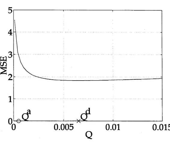
3.1 MSE of EKF frequency estimate versus

Qd

... 74

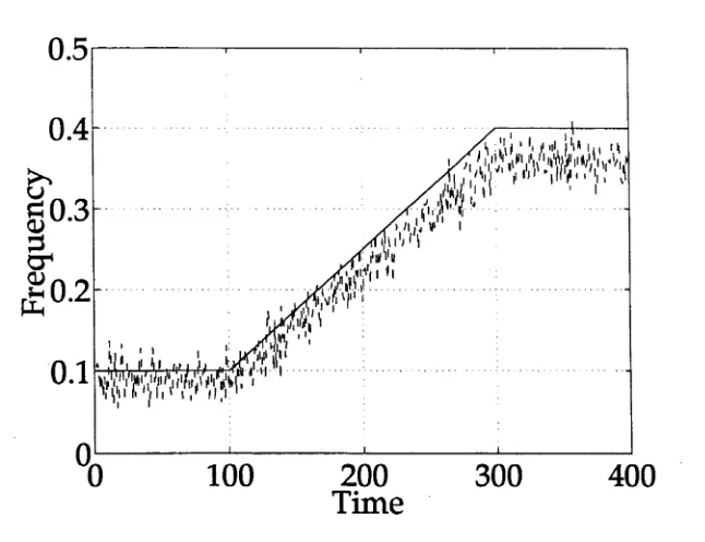
3.2 EKF frequency estimate when

Qd = Qa,ed

= ea and

Rd

=

Ra.

The target

signal is given by the solid line... 74

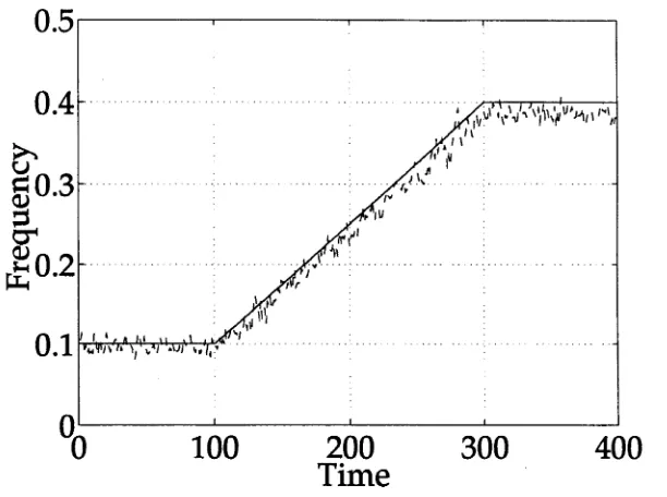
3.3 EKF frequency estimate when

Qd

>

Qa, ed =

ea and

Rd = Ra.

The target

signal is given by the solid line... 75

3.4 EKF frequency estimate when

Qd

>

Qa, ed < ea

and

Rd = Ra.

The target

signal is given by the solid line... 75

3.5 EKF frequency estimate when

Qd > Qa, ed < ea

and

Rd > Ra.

The target

signal is given by the solid line... 76

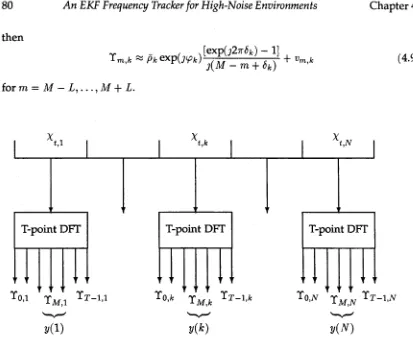
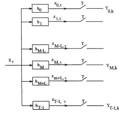
4.1 Transformation of input signal... 80

4.2 Filter bank representation of input signal pre-filtering... 81

4.3 Constant velocity sonar tra c k in g ... 89

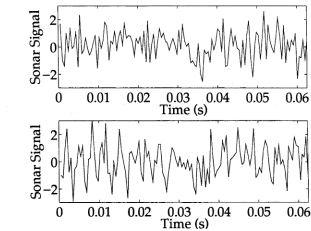
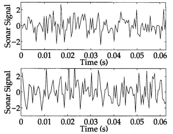
4.4 Measured sonar signal when target at greatest range (top) and closest

range (bottom) for data set 1... 93

4.5 EKF estimates for data set 1. True values given by solid line... 93

4.6 The error in the EKF estimates for data set 1... 94

4.7 Measured sonar signal when target at greatest range (top) and closest

range (bottom) for data set 2... 94

4.8 EKF estimates for data set 2. True values given by solid line... 95

4.9 Error in the EKF estimates for data set 2... 95

4.10 Measured sonar signal when target at greatest range (top) and closest

range (bottom) for data set 3... 96

4.11 EKF estimates for data set 3. True values given by solid line... 96

4.12 Error in the EKF estimates for data set 3... 97

5.1 Adaptive control for vibration rejection... 100

5.2 Oscillator+Compensator form of Vibration Control S T R ... 116

5.3 Plant output using the BNM (top) and EFRA (bottom) RLS algorithms for

Example 1...120

5.4 Estimates of controller numerator polynomial coefficients for Example 1.

True values given by solid lines... 121

5.5 Estimates of controller denominator polynomial coefficients for Example

1. True values given by solid lines... 121

5.6 Magnitude response for limiting adaptive controller (dashed line) and

ideal controller (solid line) for Example 1... 123

5.7 Phase response for limiting adaptive controller (dashed line) and ideal

controller (solid line) for Example 1...123

5.8 Parameter estimates for Example 2...124

5.10 Magnitude response for limiting adaptive controller (dashed line) and

ideal controller (solid line) for Example 2...126

5.11 Phase response for limiting adaptive controller (dashed line) and ideal

Introduction

1.1 Problem Description

J N many problems in both control and signal processing the frequency of some signal

encodes important information. One obvious example is an FM radio signal where

information is transmitted via modulation of the carrier frequency. In radar signal

processing the aim is to recover information on the velocity and range of a target from

the doppler shift in the reflected microwave signal. Monitoring the changing frequency

of the waveforms produced by rotating machinery can yield information on the rate

of mechanical wear, as well as providing measurements which can be used to control

the plant via a feedback mechanism. Improvements in efficiency and pollution control

and the elimination of "knocking" in internal combustion engines requires just such

processing (Böhme and König 1994).

Like many interesting open problems, estimating the frequency of a sinusoidal signal

in noise is not an easy one. Systems which output periodic signals have the curious

feature of being neither stable (in the sense of Lyapunov) nor unstable (in the sense of

Lagrange). Once such a

critically stable

system has been set going it will continue to

output the same sinusoidal signal forevermore, neither diminishing nor expanding in

amplitude. Typically, oscillations result from nonlinear systems but their high energy

fundamental modes are best modelled, analysed and controlled using critically stable

linear systems.

Such systems are awkward, in-between cases which are often ignored. It is not un­

common to encounter estimation or control algorithms which consider the two cases

of asymptotically stable or unstable systems, but which neglect the third, troublesome

case of critically stable systems. The reason control and estimation methods based on

Lp

optimisation face difficulties when dealing with critically stable systems and periodic

signals is that the cost function is not continuous with respect to the parameters. If a

sinusoid is not precisely accounted for, then its energy contribution to the cost function

is infinite. If it is correctly accounted for then it does not contribute to the cost func­

tion. For this reason

Lp

gain methods such as LQ, least squares and

H

oo all experience

difficulties.

The problem of estimating the parameters of a constant frequency sinusoid in noise can

be posed in a number of ways. It can be written as a linear, state space problem as

follows

Xl(fc + 1 )

cos(u>) - sin(w)

x\{k)

x2(k +

1)

sin(w)

cos(ic>)

X2 (k)

Vk

x\(k)

x2{k)

+

e(k).

Alternatively, it can be posed as the following input-output problem

y(k)

= 2 cos

{u)y(k

- 1) -

y(k - 2)

+

e(k).

Firstly, consider estimating the parameters, {a;}, of the auto-regressive (AR) model

y(k) = a\y(k - 1) + a2y(k - 2) + . . . a ny(k - n) + e{k)

where E[e(k)] = Oand E[e(k)2} = 1. This can be written as the linear estimation problem

y(k) = 4>{k - \ ) T0 + e(k) (1.1)

where

f = [ a i , a2, . . . , a n]

<t>{k-\)T = [y(k - l ) , y ( k - 2), . . . , y(k - n)].

It can also be written in state space form as

0{k + 1) = 9(k) (1.2)

y(k) = <p ( k - l ) T0(k) + e(k). (1.3)

The recursive least-squares (RLS) equations for (1.1) and the Kalman filter equations for (1.2)—(1.3) are identical since both estimation algorithms calculate the least-squares estimate of 0. Both algorithms are given by the set of equations

9(k + 1)

K(k)

P(k + 1)

9(k) + K( k) (y(k)- 4>(k)T0(k)^

P(k)<p(k) 4>(k)T P(k)4>(k) + 1

_

p(k)mmTP(k)

1 ' 4>(k)T P(k)4>(k) + 1

The inclusion of a zero mean noise term,

w(k

) with variance

Q,

in the state equation

(1.2), or equivalently modifiying the RLS algorithm to prevent Urn

K(k) =

0, will

k—

*oc

alleviate this lack of robustness for most AR models. The cases where this performance

1

improvement will not occur are those where

[F,Q2]

has uncontrollable modes on the

unit circle. The lack of uncontrollable modes on the unit circle is a necessary condition

for the maximum limiting value of

P(k

) to be non-zero (de Souza

et al.,

1986). Thus, the

inclusion of dither or noise in the state dynamics of the frequency estimation problem

will not eliminate the lack of robustness of estimators using a least-squares criterion.

Another problem in least-squares frequency estimation is that of bias. This is more

clearly seen when considering the input-ouput formulation of the problem. When esti­

mating the parameters of an AR model with unit circle zeros, equation error estimation

algorithms, such as recursive least squares, will yield biased solutions (Mendel, 1973;

Johnson, Jr. and Hamm, 1979). Moreover, in the case of constant frequency estimation,

the bias is a function of the unknown parameter,

a\ -

2 cos(u;) (Johnson, Jr. and Hamm,

1979), which makes it difficult to eradicate.

When we extend the frequency estimation problem from merely estimating the param­

eter 2 cos(u;), to estimating directly the frequency of the periodicity,

our task becomes

more difficult still as the problem is now nonlinear. If the frequency varies with time

the difficulty of the problem increases yet again. When there is more than one periodic

component in the measured signal the issues of identification of the correct number of

tones and the separation of tones closely spaced in frequency must also be taken into

account. Sometimes it is not possible to measure the sinusoidal signal directly but only

the combination of the sinusoid and some other signal. In fact, the sinusoid may be

considered a disturbance corrupting the desired output signal.

vibration control problem. In both cases, methods based on a least-squares criterion will

be used.

In spite of the difficulties in estimating the constant frequency of a sinusoidal signal, the ubiquity of the frequency estimation problem has spawned a myriad of techniques to deal with it. For high signal-to-noise ratio (SNR) regimes simple, non-parametric methods such as those based on counting the zero crossings of the signal can be used. For signals with a lower SNR there is a range of more sophisticated techniques which make use of the peculiar features of a particular frequency estimation problem to improve performance. For the case of the frequency tracking problem there are fewer options. In both cases, the choice of which method to employ depends to a large degree on the nature of the given problem to be solved.

The next section gives a brief overview of the common methods used for tracking the frequency of a single sinusoid in n o ise1. Following this is an overview of the problem of designing adaptive controllers for linear, time-invariant plants that converge to optimal controllers. The final section gives an outline of this thesis, detailing the problems considered and the proposed methods of solution.

1.2 Common Frequency Tracking Algorithms

Probably the best known application of frequency tracking techniques is that of the demodulation of FM signals using the phase-locked loop (PLL). The application of the PLL to demodulation appears to have begun with Appleton (1922). Since it was first proposed the analog PLL has been extensively studied, see for example Viterbi (1966) or Gardner (1968). Somewhat more recently digital implementations of the PLL have also been examined (Kelly and Gupta, 1972; Polk and Gupta, 1973).

Another popular technique for frequency tracking makes use of hidden Markov models (HMMs). In this approach, at any instant the system is assumed to take one of a discrete, finite set of frequency values. The probability of the system taking on a value

in the set at a given time instant is assum ed to depend solely on the state of the system

(i.e. frequency value) at the previous instant, hence the problem is Markovian. The

m easured output signal of the system is the sinusoid corrupted by channel noise. The

HMM frequency tracker was introduced by Streit and Barrett (1990). In their algorithm

the measurem ent sequence was also assum ed to take on values from a finite set of

discrete outcomes. This work has been extended by Barrett and Holdsworth (1993) to

the case w here the m easured outp u t is a continuous variable. The relationship between

HMMs and neural netw orks has been explored by Adams and Evans (1994) and a neural

netw ork based frequency line tracker proposed. H idden Markov model techniques are

clearly best suited to frequency tracking problems where the set of possible frequency

values is naturally discrete, such as the case of frequency-shift key (FSK) m odulated

signals. These m ethods are also applicable to cases where it is known that the frequency

will vary in some given range such as in the case of sonar tracking. In such cases the

frequency variable can be discretized to an appropriate degree of accuracy.

For signals whose frequency varies slowly enough with respect to the sampling rate that

the frequency can be considered constant over a reasonable time period, such as sonar

signals, it is possible to use block frequency estimation techniques. In this approach,

the signal is divided into possibly over-lapping segments and the signal characteristics,

including frequency, are treated as constant w ithin blocks. A frequency estimation algo­

rithm is then used on each subsequence. Such algorithms include maximum likelihood

m ethods (Quinn and Fernandes, 1991; Starer and Nehorai, 1992), methods based on the

Fourier coefficients of the blocked signal (McMahon and Barrett, 1986; Quinn, 1994) or

w eighted linear predictor estimators (Lankef al., 1973; Kay, 1989; Lovell and Williamson,

1992; Clarkson et al., 1994).

A nother approach, widely discussed in the literature, is that of the use of time frequency

representations (TFRs). The aim of this approach is to display the energy of the signal

as a function of both time and frequency in the m anner of a joint probability density for

a bivariate random variable. The first mom ents of such representations can be used as

estimators of instantaneous frequency. Unfortunately, it has been shown (Lowe, 1986)

that such a joint probability density as a function of time and frequency does not exist.

densities is term ed a time-frequency distribution (TFD). Such TFDs have spurious cross

term s which imply that there exists energy in the signal where there is none. The use

of TFRs for spectral analysis has been examined by Lovell (1990). It has been shown

that the most appropriate TFR for this use is simply the short time Fourier transform

(STFT) (Lovell et al., 1993). In the case of the S IF T the spurious cross terms coincide with

the true peaks in the TFD, thus distorting the m agnitude but not the location of these

peaks. O ther Cohen-class TFDs do not have this property. Moreover, it has been shown

that estimators based on the moments of common TFDs are arithmetically equivalent

to those produced by weighted linear predictor methods, are computationally more

complex and have a higher variance (Kootsookos et al., 1992; Lovell and Williamson,

1992). Thus TFRs, other than the short-time Fourier transform, are of little practical use.

One more technique for constructing frequency trackers, and indeed observers for non­

linear systems in general, is that of using an extended Kalman filter (EKF). As the name

implies, the EKF is an extension of the well-known Kalman filter, which may be applied

to linear systems, to the case of nonlinear systems. Briefly an EKF estimate is obtained

by linearising a nonlinear state space model about the current state estimate and then

producing an u p d ated state estimate using the gain calculated from a Kalman filter

on the resulting linearised system. While the EKF no longer possesses the optimality

properties of the Kalman filter it is still a valuable technique. A derivation of the EKF

and an example of applying it to the frequency tracking problem is given in Anderson

and Moore (1979, C hapter 8). A more extensive examination of the EKF for frequency

tracking is given in Parker and Anderson (1990). The performance of an EKF for both

single and m ultiple tone frequency tracking is analysed using averaging analysis by

James (1992).

1.3 Self-Tuning Regulators

Consider the problem illustrated in Figure 1.1 where there is a plant, P, the output of

which is perturbed by some disturbance process characterised by H. Suppose the plant

and disturbance process are parameterised by some unknow n vector 9°. The aim is to

an adaptive controller,

which will reject the disturbance,

and make the output of

the plant,

track some reference trajectory,

Figure 1.1: Disturbance rejection via adaptive control.

There are several questions to be answered in such a problem.

Stability

The first and foremost question is that of stability of the closed-loop system.

Is the computed control input, {tijt}, bounded and does it produce a bounded

output,

Convergence

The next question to consider is do the parameter estimates

converge

to some limiting value

Self-Optimisation

If the parameter estimates converge, does the limiting adaptive

controller,

satisfy the performance measure for the control law? If so, the

system is said to be self-optimising.

Self-tuning

If, in addition to satisfying the performance criterion, the adaptive con­

troller,

converges to the optimal controller,

then the system is said to

be self-tuning.

Consistency

If lim

then the parameter estimates are consistent and the

Systems which are self-tuning when the reference trajectory, {yj.}, is identically zero are

term ed self-tuning regulators. When the reference trajectory is non-zero they are termed

self-tuning trackers.

The problem, as stated above, is impossibly general. Even w hen the problem is restricted

to particular types of systems, control laws and estimation methods the problem is still

very difficult. A well-known example of a self-tuning tracker was first proposed by

Äström and W ittenmark (Äström and Wittenmark, 1973; Äström et dl., 1977). They

posed the self-tuning regulator problem for linear time-invariant systems described by

an ARMAX model, where the plant, P, was stably invertible and the disturbance transfer

function, H, was stable. They employed a certainty equivalence minimum-variance

controller and estimated the unknow n system param eters using recursive least-squares.

Experimental results suggested that this system was self-tuning. However, even for this

very particular form ulation of the self-tuning problem, the question of w hether Äström

and W ittenm ark's self-tuning regulator (STR) was accurately nam ed remained open for

almost 20 years.

In order to obtain answ ers to the questions above a simplified version of Äström and

W ittenm ark's self-tuning regulator was first examined. Goodwin et al. (1980) showed

that, for deterministic systems (that is w hen Vk = 0 for all k) and w hen the stochastic

approxim ation algorithm was used in place of recursive least-squares, the system was

stable and self-optimising. Bittanti et al. (1990) showed that this form of the STR was

stable and self-optimising as a regulator and as a tracker w hen the param eter estimation

was perform ed using any one of a family of recursive least-squares based algorithms.

The first result for stochastic systems (that is with a non-zero, random disturbance

{vk}) was that of Becker et al. (1985). They showed that the form of the STR which

used the stochastic approximation estimation algorithm in place of least-squares was

a convergent and stable self-tuning regulator. They also showed that the param eter

estimates were not consistent but converged to a random multiple of the true param eters

w hen the optimal controller was irreducible.

The STR as posed by Äström and W ittenmark was eventually shown to be convergent,

approaches. It was also shown that the param eter estimates will be consistent, and

hence the STR self-tuning, if the optimal controller is irreducible (Radenkovic, 1990;

Guo, 1993).

The problem posed by Äström and W ittenmark has now been extended to consider Un­

ear, time-invariant systems, least-squares estimation and a variety of control strategies.

Becker et al., Radenkovic and Guo used stochastic Lyapunov functions and Martingale

theory in their solutions. Kumar (1990) used an alternative method of Bayesian em bed­

ding (Stemby, 1977; Rootzen and Sternby, 1984) to show that the recursive least-squares

algorithm, w hen used in closed-loop, w ould converge and be consistent, independently

of the control strategy used except for an exceptional set of 0° with Lebesgue measure

zero. Moreover this result did not require assum ptions on the transfer functions of the

plant, P, and disturbance process, H, other than those of linearity and time-invariance.

Thus it is possible to show that the STR is a self-tuning regulator and tracker for a variety

of control laws provided the true system, 6°, is not in the exceptional set. Unfortunately,

the param eters for a system which has poles on the unit circle, such as systems with a

sinusoidal disturbance, lie in this exceptional set (Nassiri-Toussi and Ren, 1994).

1.4 Thesis Outline

This thesis considers frequency estimation in both open and closed loop. Firstly, it

examines the use of the extended Kalman filter (EKF) to estimate the time-varying

frequency of a noisy sinusoidal signal. The closed loop problem considered is that of

eliminating a sinusoidal disturbance from the output of a linear, time-invariant plant.

This thesis concentrates on the use of the extended Kalman filter for frequency tracking

as the EKF is one of the most flexible tools for this task. By the suitable construction

of a state space signal m odel (and possible pre-filtering of the m easurem ent signal)

an EKF tracker can be designed for a w ide variety of frequency tracking problems.

Before the EKF can be used intelligently it is necessary to understand the modes of

failure of the EKF and their causes. Accordingly, in C hapter 2 the EKF is presented

of this chapter is then concerned with presenting a new stability result for the EKF

w hen applied to discrete-time, stochastic systems which have nonlinear state dynamics.

This theorem gives sufficient conditions for the boundedness of the errors of the EKF

given a sufficiently good initial state estimate. As a corollary, this result also gives

conditions under which the errors of the EKF will converge to zero when it is applied

to a deterministic, discrete-time nonlinear system.

In Chapter 3 a general EKF-based frequency tracker is presented and general, ad hoc

tuning guidelines for EKF systems are given. In addition, the EKF tracker is shown to

satisfy the conditions of the result given in Chapter 2. As a result, theoretically based

tuning guidelines for the EKF frequency tracker are also derived. The performance of

this frequency tracker is illustrated with simulation results.

The flexibility of the EKF-based approach is illustrated in Chapter 4 by considering the

problem of passive sonar tracking. In this application the frequency of the acoustic

signals suffers a doppler shift which is a function of the velocity of the target. Since

the sonar detectors are passive the SNR of such signals is very low (in the range -20 to

-30 dB). General EKF-based frequency trackers are know n to suffer from a threshold

effect for signal w ith SNR below 5-6 dB (James, 1992). That is, the mean square error of

the state estimates increases dramatically below the threshold SNR value. To overcome

this problem a new state-space m odel is proposed which incorporates the particular

characteristics of sonar signals. In this way the effective SNR of the signal is increased

and the resulting EKF tracker is able to estimate the instantaneous frequency with

reasonable accuracy. Simulations illustrate the performance of this low SNR frequency

tracker.

A vibration control problem is considered in Chapter 5. The problem examined is that

of a linear, tim e-invariant plant whose output is corrupted by a sinusoidal disturbance

of unknow n frequency. The aim is to design an adaptive, feedback control system to

eliminate the disturbance and drive the plant output to zero. The adaptive control

system used is that of a minimum-variance certainty equivalence controller coupled to

a param eter estimator. This is an extension of Äström and W ittenmark's self-tuning

regulator to the case w hen the disturbance process is critically stable rather than strictly

stochastic perturbations. In this chapter a convergence proof is given for the vibration

control problem using a modified least-squares algorithm. This result shows that by

embedding the estimation problem in closed-loop, the known bias that occurs in fre­

quency estimation by this method in open-loop is eliminated and the output of the plant

can be regulated.

Stability of the

Extended Kalman Filter

2.1 The Extended Kalman Filter

J N this chapter the extended Kalman filter (EKF) is introduced and its stability is

dicussed. We wish to determine under what conditions the estimation errors in the

EKF will tend to zero

(asymptotic stability

) or be bounded for all time (

bounded-input

bounded-output (BIBO) stability).

This section is devoted to an overview of the EKF and

the derivation of its associated error dynamics. The following section reviews previous

work on the stability of the EKF. The rest of the chapter is devoted to a new result on

the stability of the EKF when applied to a stochastic, discrete-time system.

The extended Kalman filter is a tool for estimating the state of a system which is de­

scribed by a nonlinear state space model. The EKF state estimates are an approximation

to the mean of the conditional density of the state {

x(k

)} given the measurements

{y(l),...,

y(k)}.

Jazwinski (1970) derives this conditional density for both continuous

time and discrete time systems and gives several approximations to the moments of

these densities, including the EKF. He discusses the effect of the neglected terms in

these approximations but does not give any strict results.

The EKF is derived by linearising the signal model about the current predicted state

estimate and then using the Kalman filter on this linearised system to calculate a gain

matrix. This gain matrix, along with the nonlinear signal model and new signal mea­

surement, is used to produce the filtered state estimate and then an estimate of the state

at the next time instant. For a nonlinear signal model of the form

x(k + 1) = f ( x( k) ) + w(k) (2.1)

y(k) = h(x(k)) + v(k) (2.2)

where E[w(k)w(k)T] = Q{k) and E[v(k)v(k)T] = R(k), the equations for the EKF are

(Anderson and Moore, 1979, C hapter 8)

M easurem ent Update:

x(k\k) = x(k\k — 1) + Kx(k)[y(k) — h(x(k\k — 1))] (2.3)

P£{k\k) = [ I - K £(k)H£(k)\P£(k\k - l ) (2.4)

Time Update:

x(fc 4- \\ k) = f{x(k\k)) (2.5)

Pi (k + l\ k) = Fi(k)Pi(k(2.6)

where

Ki ( k )

Fi ( k )

Hi (k)

Pi(k\k - 1)Hi(k)T[Hi(k)Pi(k\k - \ ) Hi ( k ) T + R(k)}-'1

9fi_

dxj

x=x(A:|fc)

dh

dxj

x = x ( k \ k —1)

(2.7)

(2.8)

(2.9)

and x (k \ k) is the estimate of the state at time k and x (k + 1 1 k) is the prediction of the state

at time k + 1 using all the observations up to and including y(k). The matrices Pz(k\k)

and Pf (k + 1 \k) are approxim ations of the respective state estimate error covariances. 1

This thesis is concerned primarily with problems of frequency estimation and associated

issues and most common models for systems with time-varying frequency are linear in

either the output m ap (2.2) or state dynamics (2.1). Thus for the rem ainder of this chapter

only systems w ith a linear output map, i.e. systems with y(k) = H( k ) x ( k) + v( k) are

considered. Stability for signal models which have linear state dynamics and a nonlinear

output m ap can be derived in a similar fashion to the following.

Define the error in the filtered and predicted state estimates as e(k\k) and e{k\k - 1)

respectively. Thus

e(k\k) = x(k) — x(k\k) (2.10)

e(k\k — 1) = x(k) - x(k\k - l ) (2.11)

From (2.3)

e(k\k) = [I - K £(k)H{k)]e(k\k - 1) - K £(k)v(k)

where

e(k + l\k) = f ( x ( k ) ) + w ( k ) - f(x{k\k))

= f ( x( k) ) + w(k) — f ( x( k) — e(k\k))

= f (x{k)) + w(k) - f ( x( k) ) + ^~( x( k) ) • e(k\k) - Kj (x(k), -e(k\ k))

= x ( k)) • e(k\k) — Kj(x(k), — e(k\k)) -f w(k) ox

and Kj is the rem ainder term from the Taylor series expansion of / , i.e.

« /(a , b) = / ( a + b) - /(a ) - ^ ( a ) • 6.

Therefore

e(*|*) = [I - Ki ( k) H( k) ]Fx( k - l ) e ( k - l \ k - l )

- [ I - K £(k)H(k)]Kf ( x ( k - l ) , - e ( k - l \ k - l ) )

where

Fx(k) = j-(x(k)).

Thus the dynamics for the filtering error of the EKF may be written as the sum of the

error dynamics for the deterministic case, neglecting linearisation errors, and nonlinear

perturbation terms driven by the noise processes and remainder term from the Taylor

series expansion of the nonlinearity in the signal model.

In the case of a nonlinear output map and linear state dynamics the stability of the

prediction error of the EKF needs to be examined. In such cases the prediction error

dynamics are

e(k+l\k) = F(k)[I — K&(k)Hx(k)]e(k\k-l)

+F(k)Kx(k)Kh(x(k),

- e(fc|fc-l))

- F ( k ) K x(k)v(k)

+

w(k)

where

HAk)

= |^(x(*)).

In the fully nonlinear case the filtered error dynamics are given by the equation

e(*|A?) = [/ -

Kx(k)Hx(k)]Fx(k)e(k

-

l\k

- 1)

+ [/ -

Kx(k)Hx(k)\{w(k -

1) -

Kj ( x ( k -

1),

—e(k — l\k — l))}

- K x(k){v(k)

+

Kh(x(k), —Fx(k — l)e(k — l\k — l) + Kf(x(k — l ) , —e(k — l\k — l ) ) — w(k))}.

From this equation it can be seen how the linearisation error in the state dynamics,

n

/,

inflates the apparent noise in the state dynamics. Similarly, the error in the linearisation

of the output map,

Kh,

inflates the contribution due to "noise" in the output equation.

It can also be seen how the smoothness properties of the nonlinear functions, / and

h,

of the Kalman filter. However, note that for the fully nonlinear case, the remainder terms

are also effected by the state noise due to the presence of a w(k) term in the argum ent

of Kh. Thus in this case the degree of noise in the state is also crucial to the analysis.

In the next section we will review w hat is already know n about the dynamics of the

errors of the EKF. Knowledge of these dynamics is crucial to an understanding of when

and w hy the EKF will fail or be successful.

2.2 Previous Results

The extended Kalman filter is often used to design observers for nonlinear filtering

problems in spite of the fact that there are few theoretical results to indicate when such a

design will be successful. In practice it has been found that when the nonlinearities are

not significant such a design will often work but, until recently, more precise guidelines

have not been available. This was due to the nonlinearities and dependence of the gain

calculations on previous state estimates, which make a general stability analysis of the

EKF extremely difficult.

One approach to overcoming these difficulties is to concentrate on applying the EKF to

a particular application. Any analysis of the performance of the EKF can then make use

of the structure of the application to simplify the analysis. 2

An alternative approach is to consider modified versions of the EKF algorithm (perhaps

applicable to particular classes of nonlinear functions) which are more amenable to

analysis. For cone-bounded functions, i.e. the class of nonlinear systems where the

nonlinearities are uniformly Lipschitz in the state variable, a nonlinear observer has

been proposed and analysed (Gilman and Rhodes, 1973; Rhodes and Gilman, 1975). A

bounding linear system for such systems can be found. By calculating the gain using

this nom inal linear system the dependence of the gain on previous state estimates is

rem oved and it is possible to derive upper and lower bounds for the estimation error

covariance.

Safonov and Athans (1978) considered using a constant gain in the EKF. Their motiva­

tion for a constant gain EKF (CGEKF) was primarily to reduce computational complexity,

how ever it also allowed a theoretically based stability analysis to be performed. They

derived a sufficient condition for the stability of the CGEKF and described an ad hoc,

iterative design procedure.

Song and Speyer (1985; 1986) proposed a modified gain EKF (MGEKF) for modifiable

functions, i.e. functions for which an exact expansion of f ( a + b) about (a + b) can

be found. By incorporating this expansion, rather than the first order Taylor series

approximation, in the EKF equations it is possible to derive global stability conditions for

the MGEKF. U nfortunately these conditions are not verifiable analytically. Pachter and

Chandler (1993) proposed a m ethod for deriving an approximation to the appropriate

expansion of f (a + b) for smooth nonlinearities using a M aclaurin series expansion of / .

A hm ed and Radaideh (1994) also proposed a modified EKF (MEKF). They considered

stochastic, continuous-tim e systems and expanded the nonlinearities about the solution

of the deterministic, undriven state equation. As the solution {£(<)} of

dx{t) dt

is a known, deterministic sequence it is possible to derive upper bounds on the error

between the determ inistic solution and the true state, x(t) = x(t) - x(t). Moreover the

resulting MEKF equations for (x(/)} are linear in the state given the know n sequence

{x(*)}. Thus their MEKF is the optim al linear estimator of x. The authors claim that as

E [ x (t )\ y (l ) ,. .. ,y ( t) ] ~ x(t) + x{t) (2.13)

w here x(t) is the estimate of x(t) produced by their MEKF, the MEKF is more accu­

rate than the standard EKF. H owever they make no comment on the accuracy of the

approxim ation in (2.13).

Chui et al. (1990) examine the case of using the EKF to estimate both the param eters as

well as the state of a linear system. They propose a parallel algorithm where the states

parameter estimates. This sequence of parameters estimates is produced from an EKF using the state estimates from the Kalman filter. In other words, let x\ (k ) be the estimate of the state of the system at time k and x2{k) be the estimate of the parameters of the system at time k, then x \ ( h + 1) is given by a Kalman filter run on the linear system

x \ (k + 1) = h ( x2(k))xi(k) + wi(k) (2.14)

and x2 (k + 1) from an EKF run on the nonlinear system

x2{k + 1) = f2(x\{k), x2(k )) + w2(k) (2.15)

where { tx;i(A:)} and {w2(k)} are white noise processes. The authors claim that as the estimates of {x-[(k)} given by the Kalman filter run on the system (2.14) are the optimal estimates of x\(k) given { y [ l ) , .. . , y ( k) , x2( l ) , .. . , x 2(k)}, the estimates given by the coupled system (2.14)-(2.15) will be more accurate than those given by the standard EKF. This is due to the fact that the linearisation about x\(k) in the EKF for the system given by (2.15) will be more accurate than the linearisation about the generic EKF estimate of x\ since x\(k) is the optimal estimator of x\.

The first theoretically based analysis of the standard EKF in a reasonably general setting arose from Ljung's examination of the EKF as a parameter estimator (Ljung, 1979). He examined the asymptotic behaviour of the EKF when it is used to estimate the unknown parameters, as well as the state, of a linear, time-invariant system. The analysis was performed by approximating the dynamics of the errors in the EKF estimates by an ordinary differential equation and examining the limiting points of this equation. He concluded that, in general, the parameter estimates given by the EKF would be biased due to errors in modelling precisely the noise structure of the system. He proposed a modified algorithm, based on stochastic gradient descent arguments, which has improved convergence properties. The modifications are similar to the ad hoc process of tuning the EKF by varying the noise covariance matrices. 3

More recently there have been several attem pts to quantify the performance of the EKF

for general nonlinear problems. Baras et al. (1988) have given conditions under which

the EKF will be a locally asymptotic observer w hen applied to a deterministic, continu­

ous time system. That is, they have shown that the errors in the state estimates will tend

to zero if the initial error is small enough under appropriate conditions. Following from

the w ork in Baras et al. (1988), Song and Grizzle (1993) have dem onstrated a similar

result in the discrete time case. In addition Picard (1991) has considered the case of ap­

plying the EKF to continuous time, stochastic systems w ith high signal-to-noise ratios.

He gives conditions un d er which the scaled EKF filtering error will be asymptotically

optimal and provides a bound for the EKF estimation error in terms of the SNR and

com puted error covariance.

In the following subsections the theorem s of Baras et al. (1988), Song and Grizzle (1993)

and Picard (1991) are given and then briefly discussed.

2.2.1 Deterministic, Continuous Time Systems

Baras, Bensoussan and James (1988) examined this case. Their results were the following.

Consider the deterministic, nonlinear, continuous time system

x(t) = f (x(t )), x(0) = xq

y(t) = Hx(t )

The extended Kalman filter for such a system is given by the equations

rh(t) = f ( m( t ) ) + N ( t ) H T R ~ l [y(t) — Hm(t)], m(0) = mo

N(t ) = ^ - ( m ( t ) ) N ( t ) + N ( t ) ^ - ( m ( t ) ) - N ( t ) H TR - ' H N ( t ) + Q,

N(0) = N0 = P g l

Definition 2.1 The pair [H. F{x)] is uniformly detectable if there exists a bounded Borel matrix-valued function A(x ) such that

t1T ( F (x) + A( x ) H )r) < —ck0|/7I2, q0 > 0

for all x,rj E 1R!.

Definition 2.2 The pair [F{x), Q] is uniformly controllable if there exists a bounded Borel matrix-valued function T(x) such that

\ T( F( x) + Q T ( x ) ) X > ß 0\ \ \ 2, ß 0 > 0

for all x, A E lRn.

Theorem 2.1 (Theorem 7, (Baras et al., 1988)) If

1. [ R~2H, |£ (x)] is uniformly detectable; and

2. [ |i i x )i Q] is uniformly controllable

then

I W O I I <

A

mm =

<

A

\ m +

q

I I Q 5II2 + | | A | | :

2uo

l|Ar-1(Oll

\ \ m +

p

p - ^ l l 2 + lir||:

2ß0

l|A|| = sup ||A(x)|| x£Rn

||r||

Theorem 2.2 (Theorem 8, (Baras et al., 1988)) Assume

1. f : IRn —► IRn is smooth with bounded first derivative;

2. Q > qol for some go > 0;

3. [R~2 H, |£(x)] is uniformly detectable;

4. [§£(*), Q] is uniformly controllable; and

5. [H, |£(®)] is uniformly detectable.

If

where

then

|*o - m0|||d2/|| < max

₁

_J

n2p 2||F02 ||

||ö2/|| = sup ||§ 4 ( * ) ||

|* (0 - m ( t)I < C|x0 - m0| exp(—7<)

for all t > 0 for some constants C > 0,7 > 0.

(2.16)

2.2.2 Stochastic, Continuous Time Systems

Picard (1991) examined this case when the system has small noise. Consider the non­ linear system

d x t = f ( t , x t )dt + \A g (t, x t )dwt + y/eb(t, x t )dvt

dyt = h(t, x t)d t + \fkdvx

where wt and vt are independent Brownian motions. The extended Kalman filter for this system is given by the equations

m t = m0 + [ f ( s , m $)d s+

f

Jo Jo

P,

[F(t)-+ Pt[F(t) - +

where

H ( ! ) =

Fit)

Make the following definitions.

D efinition 2.3 A function f ( t, x, e) is almost linear i/ f/zere exists afamily of matrix valued processes Ft(e) such that

\ f ( t, x, e) - f ( t , m , e) - JF<(e)(x - m)\ < p t \x - m\

for some family of numbers p t —► 0 as e —*■ 0.

D efinition 2.4 function f i t , x) is strongly injective if

\ f ( t, x) — / ( t , m)| > c|x — m|

for some c > 0.

The following result can then be obtained.

Theorem 2.3 (Theorem 2.2.1 (Picard, 1991)) Assume

1. the functions g and b are bounded;

2. the functions f and h are C 1 and almost linear;

3. the function h is strongly injective;

4. ggT is positive definite; and

v

then

for all t >

0.

_ l

P0 2(zo - rn0) = 0(y/c)

_ 1

Pt 2(xt - m t ) - 0(y/e)

2.2.3 Deterministic, Discrete Time Systems

Song and Grizzle (1993) have examined this case. Consider the nonlinear, single-input

single-output system

x { k

1) =

unknown

y{k) = h(x(k)).

The extended Kalman filter for this system is given by the equations

x ( k\ k

) =

— 1) +

(k)(y(k) —

—

1)))

p ^ ifc)-1 =

x(k

-f 1|&) =

P(* + l|*) =

+

K

=

-

1

+

where

m

=

Make the following assumptions

1. There exist ß \ , > 0 such that

k

ß i l < Y H h k ) TH(k)R-^H(k)^(i , k) < ß2I i = k —M

for some finite M > 0 and for all k > M where

$(*;, i) = F(k - 1 )F(k - 2) • • -F(*);

2. ^ -( s ) is non-zero for each a: G 1R;

3. The following bounds exist and are finite

\F

sup|T(x)|

X

\F-'\ A

s u p l^ x )-1!

X

|H| A

s u p |i r i £ ( * ) |

, d 2 f , A \ d 2f ,

..

—

S“P f e WI

d 2h A t d 2h ,

„

d x 2

S"P

4. Let

g{x, y) = /i(r) - A(x) - ^ ( r ) ( x ~ y)

and suppose there exists c < 00 such that

1 / \ 1 . d h 11 . 2

|yO,y)l < q ^ H x - yl

Theorem 2.4 Given the above assumptions there exists p ,q ,r , 6> 0 such that

|P(fc|fc)| < \P(k\k —1)| < q

\P(k\k — 1)-1 | < p

\P {k\k)~l + F (k )Q ~ 'F (k )\ < r \K(k)\ < 6

for all k > 0.

Theorem 2.5 (Theorem 3.2 (Song and Grizzle, 1993)) Consider the filtering error, e ( k) = x (k ) - x(k\k - 1), then if|eo|, \ ^ i \ and | ^ | are such that for some7 > 0

1 1 d2f

V(q-2V(

0,e0)2 ,|^ |

dx2I) < - 7

where

then

V ( k , e ) = eP (k\k —l ) - 1 e

<^>(e,X,Y) = 6 c Y l F | + \X { p q + bcYe)2

<p(e,X,Y) = = \ + pe<f,(e,x,Y)(2pq\F

lim e(k) = 0.

k— * 00

2.2.4 Discussion

There are a num ber of common features shared by these three results. As would be

expected they all require limits on the size of the nonlinearities (condition 1 and equation

(2.16) for Theorem 2.2, conditions 1 and 2 for Theorem 2.3 and condition 3 for Theorem

2.5). This is a result of the fact that the derivation of the EKF is based on the assumption

that the neglected, higher order term s in the Taylor series expansion of the nonlinearities

initial error be sufficiently small. Once again this is a result of the assumption that the

linearisation of the signal model is sufficiently good. As this can only be true within a

sufficiently small region, a global stability result for the EKF would not be possible.

In addition to conditions imposed by the assumption made when deriving the EKF all

three results require that the nonlinear system satisfy global observability and controlla­

bility style conditions (conditions 3,4 and 5 for Theorem 2.2, condition 3 for Theorem 2.3

and condition 1 for Theorem 2.5). Such conditions are restrictive. In particular, signal

m odels for the frequency tracking problem cannot satisfy global observability condi­

tions as the sine and cosine functions are not one-to-one mappings. However these

conditions can be weakened as they are not fundam ental consequences of assumptions

m ade w hen deriving the EKF.

In this rest of this chapter the remaining case of the performance of the EKF when applied

to a discrete time, stochastic system is considered. (Note only the case of systems

w ith nonlinear state dynamics but a linear output map is examined.) In addition to

completing the set of results given by Baras et al. (1988), Song and Grizzle (1993) and

Picard (1991), this result weakens some of the restrictive conditions required by previous

stability analyses. In particular, the key assumption of uniformity in the bounds on the

grow th rate of the nonlinearities and of observability properties of the signal model used

in Theorems 2.2, 2.3 and 2.5 is relaxed. In addition, an assumption of high signal-to-

noise ratios is not made. Instead, the effect of the size of the noise is included explicitly

in the sufficient conditions for bounding the filtering error of the EKF.

In obtaining this nonlinear perturbation result it is necessary to examine not only the

dynamics of the estimator but also of the associated Riccati difference equation. The

result obtained shows that the stability of the error systems depends, as w ould be

expected, on the nature of the nonlinearities and the size of the noise processes. These

2.3 Nonlinear Stability Theorems

2.3.1 Norms and Notation

Before presenting the required stability theorems it is necessary to define precisely the

notation to be used in the rem ainder of the chapter.

Definition 2.5 Let | • | be some vector norm then the corresponding induced matrix norm is denoted by

11A11 = sup I Arc I kl=i

where A is a matrix and x is an appropriately sized vector.

Definition 2.6 Let | • | be some vector norm then the correspondinginduced tensor norm is denoted by

\\B \\= sup \ B x i . . . x n \

|xi|,...,|xn | = l

where B is a tensor of degree n and x\ , . . . , x n are vectors of appropriate lengths.

A property of induced matrix and tensor norm s is that they are sub-multiplicative, i.e.

\ \ m <

pupil.

The required nonlinear stability theorem s involve the use of derivatives of vector valued

functions. In the following a short-hand notation will be given for these derivatives and

some chain rules for derivatives of these quantities will be derived.

Definition 2.7 Let a column vector of length n be written as

v = [vi\, z = l , . . . , rc

Definition 2.8 Let an n x m matrix be written as

O

il _{i = l , . . . , n j = 1, . . . , m}

where A l3 is the (i, j)-th element.

Definition 2.9 Let an n x m x r tensor be written as

B = [Bijk], i = l , . . . , n j = 1 , . . . , m =

where BXJk is the (i, j, k)-th element. Let higher order tensors be defined similarly.

Definition 2.10 Suppose f : lRn —<• Rm then

1.

dj_ A . dfj

dx dxj

2.

d2f a f d fi d x2 dxjdxk

3.

d3f a . d fi dx3 dxjdxkdxi

for i = 1 , . . . , m and j , k , l =

Definition 2.11 Suppose A : R r - ^ Rnxm then

dA a r d A i j

dx dxk

/or i = 1 , . . . , n, j = 1, . . . , m and k = 1, . . . , r

Lemma 2.1 Consider y = A ( x ) x where y is a p x 1 vector, x is a n x 1 vector and A i s a p x n

m atrix which is a function of x, then

d y , d A ( x )

JT = A (x + —f h Lx

Proof

Immediately from the definitions

dy%

d x j — ( ^ 4(x),fcXfc)

h { ) h

£ A ( x ) ik( ]k + £ ^ ^ x k k=1 k=1 d x j

for i =1 , . . . , p and j = 1 , . . . , n, therefore

dy_

d x = A ( x ) + d A ( x )

dx X

Lemma 2.2 Consider C ( x ) = A ( x ) B ( x ) where x is a n x 1 vector, A is an r x p matrix and

B is a p x m m atrix then

d C _ d A d £

d x d x d x

Proof

Again from the definitions

d c = dCjj

dx dxk

for i = 1 , . . . r, j = 1 , . . . , m and k = 1 , . . . , n where

dCjj

d x k ■ ^ ( J 2 A (x '>itB(x h )

± dJ§ r B h + ± A ü

l—\ UXk /=!