Functionality and Expanding Applicability
Michael Brown
A thesis submitted for the degree of Masters of Philosophy of The Australian National University
This thesis contains no material which has been accepted for the award of any other degree or diploma in any tertiary institution, and to the best of my knowledge and belief, contains no material previously published or written by another person, except where due reference is made in the text of the thesis.
Michael L. Brown
All experimental measurements contained within this thesis were done using the Australian National University Heavy Ion Accelerator. These measurements were undertaken with members of the Nuclear Reaction Dynamics and/or the Nuclear Structure groups, assisted by the department and school technical staff.
Analysis was performed using software developed by myself – either on top of the ROOT framework or standalone – with suggestions and input from Professors David Hinde and Nanda Dasgupta.
Michael L. Brown
The potential of gas-filled solenoids for separating fusion reaction products produced using particle accelerators has recently been realized at the Australian National University. Their capability of high efficiency transportation of fusion products and beam particle suppression means that they can be used to measure fusion cross-sections with better precision than practically achievable with other separating mechanisms. In order to effectively configure and use these solenoidal separators, simulation of the ions paths is required to determine and optimize the transmission of the fusion products.
This thesis discusses the physical processes that need to be taken into account when doing this simulation, and describes the code Solirte developed to perform the simulations. Since the simulation requires following the trajectories of a large number of ions, the implementation of the simulator on commodity graphics cards (in order to substantially increase the performance) is described.
The interactions between the high-speed heavy ion and the gas filling the solenoid depends on the mean charge state, which is typically taken from empirical models. Increased accuracy in these values will give an increased accuracy in the final results. A self-consistent approach is therefore developed in this thesis to derive the mean charge state and initial angular distribution of the fusion products. The simulator support and experimental analysis methods required to perform these techniques are described and applied to the 58Ni +64Ni fusion reaction.
Declaration iii
Contributions v
Abstract vii
List of Tables xii
List of Figures xiii
1 Introduction 1
1.1 SOLITAIRE . . . 1
1.1.1 The reaction . . . 1
1.1.2 Detecting the products . . . 2
1.1.3 Suppressing the direct beam . . . 2
1.1.4 Suppressing elastically scattered beam-like particles . . . 2
1.1.5 Separating the fusion products . . . 5
1.1.6 Additional details . . . 5
1.2 Detecting fusion reaction products . . . 6
1.2.1 Single multi-wire proportional counter . . . 7
1.2.2 Two multi-wire proportional counters . . . 8
1.2.3 Silicon detector . . . 8
1.2.4 Vetoing of elastics . . . 9
1.3 The need for simulation . . . 10
1.4 Thesis overview . . . 11
2.1.1 Solenoid focusing . . . 13
2.1.2 Magnetic field file . . . 14
2.2 Gas interactions . . . 15
2.2.1 Scattering . . . 15
2.2.2 Charge exchange . . . 16
2.2.3 Energy loss . . . 18
2.2.4 Energy interpolation . . . 19
2.2.5 Input parameters . . . 19
2.3 Initial ion properties . . . 20
2.3.1 Beam profile . . . 21
2.3.2 Angular distribution . . . 21
2.3.3 Energy distribution . . . 23
2.4 Conclusion . . . 23
3 Simulator optimization 25 3.0.1 GPU execution architecture . . . 26
3.0.2 Integration of a time interval . . . 28
3.0.3 Implementation details . . . 30
3.0.4 Performance results . . . 32
4 Image size and transmission 35 4.1 Monitor normalization . . . 35
4.2 Transport efficiency . . . 36
4.2.1 Scanning of the magnetic field . . . 37
4.2.2 Point of closest approach . . . 39
4.2.3 Minimum projected width . . . 40
4.3 Detector efficiency . . . 42
4.3.1 Intrinsic efficiency . . . 43
4.3.2 Event pile-up . . . 43
4.3.3 Acquisition system dead time . . . 43
5 Angular distributions of ERs from the target 45 5.1 Contributing sources . . . 45
5.1.1 Angular distribution due to particle evaporation . . . 46
5.1.3 Quantities required for simulation . . . 46
5.2 Evaporation of a single neutron . . . 47
5.2.1 Angular distribution . . . 47
5.2.2 Velocity distribution at a given angle . . . 49
5.3 Evaporation of multiple neutrons . . . 51
5.4 Evaporation of charged particles . . . 54
5.5 Deducing initial angular distributions from experimental results . . . 55
5.6 Simulating with a numerical Vk distribution . . . 57
5.7 Example: 221 MeV 58Ni on64Ni . . . 59
5.8 Limitations . . . 62
6 Mixed gas operation 65 6.1 Simulating with mixed gases . . . 67
6.1.1 Simulation difficulties . . . 68
6.1.2 Equilibrium charge state distribution for multiple gases . . . 68
6.2 Experimental difficulties . . . 69
6.3 Example – 140 MeV 28Si on 124Sn . . . 69
6.4 Example – 160 MeV 34S on 168Er . . . 72
7 Conclusion 75 7.1 For further investigation . . . 75
7.2 Final words . . . 76
A Point-object distances 77 A.1 Point-cone distance . . . 77
A.2 Point-cylinder distance . . . 78
A.3 Point-hole distance . . . 79
A.4 Point-cuboid distance . . . 79
B Relaxation-based histopolation 81 C Solirte input file documentation 83 C.1 Conventions . . . 83
C.2 Input file formats . . . 83
C.2.1 Run configuration file . . . 83
C.3 Output file formats . . . 93
C.3.1 General file headers and structure . . . 93
C.3.2 Obstruction hits . . . 94
C.3.3 Ion trace . . . 95
C.4 ROOT functions . . . 96
C.4.1 Common . . . 96
C.4.2 Hit masks . . . 96
C.4.3 Event plotting . . . 97
C.4.4 Iontrace plotting . . . 98
D Solirte input files 99 D.1 Field scan for 160 MeV 34S on168Er through N2 . . . 99
D.2 Mean charge state for 221.16 MeV 58Ni on64Ni . . . 100
D.3 Final radius vs initial angle for 239.1 MeV58Ni on60Ni . . . 102
D.4 Gas mixtures for 140 MeV28Si on 124Sn . . . 103
1.1 Schematic view of a typical SOLITAIRE configuration. . . 2
1.2 The magnetic circuit of SOLITAIRE (from [4]). . . 4
1.3 Average charge state of individual ions through varying gas depths. . . 6
1.4 Diagram of the SOLITAIRE multi-wire proportional counter detectors. . . 7
1.5 Schematic of the delays as used in the MWPC detectors. . . 7
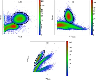
1.6 Example histograms from pairs of signals from using two MWPCs. ER events are circled. 8 1.7 Primary decay modes for known nuclei (from NuDat2[6]). . . 9
1.8 Vetoing of full energy elastics. Events in the shaded time window are not seen by the acquisition system. . . 10
2.1 Z-R and X-Y views of a typical ion path through the solenoid. . . 14
3.1 A simple warp divergence . . . 27
3.2 Four GPU integration architectures. . . 29
3.3 Flow of ion blocks for GPU processing . . . 31
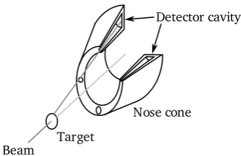
4.1 The SOLITAIRE nosecone with detector cavities. . . 36
4.2 Process for determining the image width for charge state analysis. . . 38
4.3 The geometry of the backwards raytracing. . . 39
4.4 Backwards raytracing of 239.1 MeV 58Ni on60Ni . . . 41
4.5 Focal lengths for variousqscalefactors. . . 42
5.1 Velocity spread resulting from two evaporations. . . 46
5.2 Geometry of obtaining γ values from a givenθ and Vk. . . 50
5.3 Types of domains when integrating overθ and Vk. . . 50
5.4 Vk-θ mapping forVZO= 25, normalized per-θ. . . 51
5.6 Example angular distributions (right) of an alpha (top) and alpha plus a neutron (bottom)
and the velocity distributions (left) that create them. . . 54
5.7 Input angular distributions (step-Gaussian, 1 degree step and 1 degreeσ) for reconstruct-ing Vk. . . 56
5.8 Reconstructed Vk distribution from a step-Gaussian angular distribution input. . . 56
5.9 Flowchart for simulation with an arbitrary angular distribution. . . 58
5.10 Angular-to-radial mapping for 221 MeV58Ni on64Ni. . . 60
5.11 Radial distributions of 221 MeV58Ni on64Ni, simulated (red) and experimental (black). . 61
5.12 Calculated angular distributions of 221 MeV 58Ni on64Ni. . . 62
6.1 ER image widths for 240 MeV 58Ni as a function of solenoid field on a range of targets. . 66
6.2 ER image widths for 160 MeV 34S +168Er, with various N2 gas pressures. . . 66
6.3 Detector image widths for various gas mixtures for the reaction 140 MeV 28Si on 124Sn . . 70
6.4 Detector image widths for various gas pressures for the reaction 140 MeV 28Si on 124Sn . 71 6.5 Simulated and experimental ER image widths for 160 MeV 34S + 168Er. . . 73
Introduction
Fusion reactions are of significant interest in nuclear physics because of their ability to test a wide range of physical properties and theories. The method of measurement typically involves an intermediate-energy (1 to 10 MeV per nucleon) beam of particles striking a fixed target. The resulting compound nucleus products are “hot”, and rapidly evaporate some number of neutrons, protons, and alpha particles. The resulting cooled nucleus is called an evaporation residue (ER). Due to conservation of momentum, the fusion products and the scattered beam are mixed together and require some form of separation and identification. Historically, any particular separation process tended to sit somewhere on the continuum between high acceptance of fusion products (with also high acceptance of beam particles, requiring complex detection schemes) and high suppression of beam particles (with also high suppression of fusion products, resulting in long run times for small cross-section reactions).
Solenoidal separators offer the ability to get the best of both worlds – very high acceptance of fusion products, and high suppression of beam particles. SOLITAIRE (solenoid for in-beam transport and
identification of recoilingevaporation-residues) is a fusion product separator developed at the Australian National University Heavy Ion Accelerator Facility that employs a superconducting solenoid to achieve an effective solid angle of 86 millisteradians, corresponding to an acceptance of scattering angles from 0.5 deg to 9.5 deg. This results in a transmission ratio between the target and the detectors for fusion products of typically 90%, while heavily suppressing the beam.
1.1
SOLITAIRE
Since the structure of SOLITAIRE is important for most of the following chapters, a brief explanation of the components (and the reasons behind the components) is given below. The overall structure of the SOLITAIRE is shown in figure 1.1 for reference during this explanation. A more detailed discussion of the important aspects that enable the separation of ERs from beam-like particles is given in [1].
1.1.1 The reaction
Multi-wire proportional counter detectors Silicon detector (OR)
front
Rod and stoppers: back
Solenoid coils Faraday cup
Nose cone Target
Front window
Exit collimator
Extension Back window Beam direction
Figure 1.1: Schematic view of a typical SOLITAIRE configuration.
When six targets is insufficient, there is also a small target ladder docking chamber off the main target chamber. By fully extending the linear arm, the docking chamber (now containing the target ladder) is sealed off from the main target chamber. This allows changing of the targets without requiring that the entire apparatus to be brought up to atmospheric pressure and pumped down again.
1.1.2 Detecting the products
With the beam now interacting with the targets, the next conceptual step is to discuss the fusion products. Conservation of momentum requires that these are still going in the downstream direction, so the detection apparatus is placed downstream of the target. This can either be one or several detectors (gas-filled, solid state) or more complex apparatus such as a secondary target and associated detectors for when the solenoid is being used to generate radioactive ion beams.
1.1.3 Suppressing the direct beam
While simply placing a big detector directly downstream of the target will result in most fusion products being caught, it will also result in the entire beam, both scattered and unscattered, reaching the detector. Quite apart from the damage that would occur to the detector from the beam, the beam particles outnumber the fusion products by many orders of magnitude. To eliminate the direct unscattered beam particles, a Faraday cup can be placed directly downstream from the target.
While this results in essentially complete attenuation of beam particles that pass straight through the target, it also will stop some fusion products (ERs). Because of evaporation from the compound nucleus, and scattering in the target, ERs generally have a considerable angular spread coming out of the target. By placing a small Faraday cup some distance downstream, many of the fusion products will be outside the Faraday cup, while the relatively narrow beam can still easily be caught.
1.1.4 Suppressing elastically scattered beam-like particles
The start of the solution here lies in the fact that the particles leaving the target will be charged as a result of their high velocity. When the ion comes close enough to an atom of the matter it is passing through, there is an apportunity for electrons to be transferred between the two atoms. As a result of many of these exchanges, the ions leaving the target have a distribution of charges. While the exact distribution is complex and computationally infeasible to calculate exactly, it can be closely approximated by a Gaussian of mean charge ¯q and width σ. Various empirical approximations for ¯q and σ have been developed. For the systems commonly used in SOLITAIRE, the approximation by Nikolaev[2] has been found to provide reasonable values:
¯ q=Z
1 + v Zαv0
−k1−k
(1.1)
dhwhm=d2 v u u tq¯
"
1−q¯ Z
1k #
(1.2)
where k = 0.6, v0 = 3.6×10⁶ m s−1, α = 0.45, d2 = 0.5, and Z is the nuclear charge. Note that the
half-width-half-maximum (dhwhm) needs to be converted to σ by dividing by
√ 2 ln 2.
Since the fusion products and beam-like particles are different elements, the distribution of charges on exit is different, but the momentum is the same. This combination of properties can be exploited by using a solenoid to focus the ions.
Solenoid focusing
The simplest case is an infinite solenoid which acts as a lens to charged particles emitted from a point on the axis of the solenoid. This is due to the helical path followed by a charged particle in a uniform magnetic field. Taking the solenoid axis to be the z axis (a convention that will be used from here on), the period of rotation in the x-y plane ist= 2qBπm
Z wherem is the mass of the particle,q the charge, and
BZ thez component of the magnetic field (which, for our infinite solenoid, is simply the magnetic field).
To bring the emitted particles back to the axis (with unitary magnification), one full loop needs to be completed, requiring a z distance of 2πmvqBcosθ
Z where θ is the initial angle from the z-axis. If this angle
is kept small, then cosθ≈1. Applying a thin lens interpretation of this, and substituting p=mv, gives a focal length of qBπp
Z
Since SOLITAIRE is not an infinite solenoid, a different treatment is required. The focusing proper-ties of (finite) solenoids have been extensively studied, initially for use in cathode ray tubes and electron microscopes. In such a solenoid, the radial velocity and z-axis field still impose a helical path on the particle. However, as the particle gets further away from the z axis, the z component of the velocity and radial component of the field generate a force in opposition to the helical path. The combination of these forces once again results in the solenoid acting as a lens, this time with a focal length of[3]:
f = 4p
2
q2B¯2
ZL
(1.3)
whereLis the length of the solenoid, pis the momentum, and ¯B2
Z is the mean of the square of the axial
magnetic field, given by:
¯ B2
Z =
1 zf −zi
Z zf
zi
Bz2(z) dz
Optically,ziandzf are the object and image positions along the z axis. For a fixed field, the focal length
Figure 1.2: The magnetic circuit of SOLITAIRE (from [4]).
This second expression can be thought of as the opposite of the first – it assumes that the solenoid is very thin compared to the object-image distance, instead of the solenoid being very much longer than the object-image distance (and thus enclosing both the object and image in the field, with negligible fringing effects). A real solenoid like SOLITAIRE is somewhere in between these two extremes (rather closer to the second), with a focal point that correspondingly is somewhere between the two estimations. Consequently, neither of these expressions allow for an exact calculation of focal length, though they do allow approximate scaling of experimentally known focal lengths to similar systems.
Containment of the field
SOLITAIRE is build around a 6.5 Tesla1 superconducting solenoid. The solenoid coils themselves have an operating temperature of 3.2 K, so are superinsulated both externally and from the “warm” bore that carries the fusion products.
One potential issue with having such a strong solenoid just downstream from the target is that the fringing fields are still quite significant at the target, and even further upstream. Interference with the beam upstream from the target is undesirable. Additionally, an unshielded 6.5 T solenoid can interfere with mechanical devices such as pumps, and requires care when working on while active.
To solve these issues, the solenoid is made to be part of a magnetic circuit, as shown in figure 1.2. The two main other components of the circuit are the iron yoke providing a return path for the magnetic field, and the nose cone (see figure 1.1). The nose cone performs two tasks. The first is a further reduction in the magnetic field near the target by nearly an order of magnitude[1]. The second is to shield the path from the target to the forward-scattering detectors used for beam normalization. These detectors are discussed in section 4.
Blocking beam-like particles
Since the beam-like particles and fusion products have the same momentum but different distributions of charge out of the target, the solenoid focusing results in a different distribution of focal points along the axis. To reduce the number of beam-like particles then just requires placing obstructions along the axis where high intensities of beam-like particles are expected. There are two such obstructions in SOLITAIRE. The first is the back rod, which is a 4 mm diameter threaded rod, which typically holds
1
three discs diameter 12 mm. The back rod is intended to catch the essentially full energy beam-like particles resulting from scattering in the target.
A second rod is placed between the back of the Faraday cup and the back rod. This front rod was recently added in response to a significant number of low-energy beam-like particles still passing through the solenoid. They were identified as coming to a focus twice – once before the back rod, and once after – resulting in high transmission through the solenoid. The source of these particles has not been conclusively identified, though appear to be related to scattering off the target and some internal SOLITAIRE components. While there have been no systematic comparisons with and without the rod, comparison of reactions measured both before and after the installation of the rod indicate only a minor improvement in background, and this could also be attributable to improved beam tuning.
These rods alone are not a complete solution to the suppression problem since the beam-like particles and ERs often have overlapping charge state distributions. For example, 150 MeV64Ni ions coming from a target will have ¯q= 20.88 anddσ = 1.21. If the target is also 64Ni, then the 75 MeV128Ba(assuming
no evaporation) has ¯q = 23.13 and dσ = 1.79. Even if all ions with ¯q less than 23 are blocked (meaning
blocking nearly half the ERs), the proportion of beam-like particles getting past is still 0.013, or about 1 in every 75 beam-like particle being transmitted. This is orders of magnitudes away from what is required to avoid overloading the detection system.
1.1.5 Separating the fusion products
The solution to this problem is to fill the solenoid bore with a gas. A pressure as low as a few Torr is usually sufficient. Similar to the charge exchange interactions that occur in the target, charge exchange interactions occur as the ions pass through the gas. Assuming the distance between charge exchanges is sufficiently small, the effective charge state of any individual ion over the whole path through the gas is typically the mean charge state of the ion in the gas, ¯qgas. Crucially, the ¯qgas for fusion products is
lower than those of the beam species.
An example of this is shown in figure 1.3. Horizontal from the middle is the distance from the target, with the y position being the mean value ofq2 for each ion since leaving the target. The colors indicate intensities – red being the most ions, blue the fewest. The system being shown is for 150 MeV 64Ni on a 64Ni target, with the ions passing through 1 Torr of helium, but the general principle applies to all systems. In the middle (0 m from the target), the charge state distributions are assumed to be identical between the products and beam-like particles (and uniform overq from 0 to Z, for clarity). The discrete charge states are clearly visible in the beam-like side, where the mean free path between charge exchange events is greater. As the path length grows, the average charge over that path trends towards a common value, regardless of the initial charge. Over a two metre path length, the distributions of ¯q2for beam-like
and product particles (the far left and right of the diagram respectively) are nearly disjoint.
1.1.6 Additional details
Since the solenoid is now filled with gas, this gas needs to be prevented from going upstream of the target chamber. This is done by using thin (14 to 65 µg/cm2[1]) carbon foils to isolate the target chamber and solenoid bore from the accelerator upstream. Such foils are regularly produced via evaporation-deposition for electron stripping in the main accelerator, or for supporting weak targets. Additional care has to be taken during construction to avoid pinholes anywhere on the foil, but otherwise the process is unchanged. These foils have proven to be very robust during solenoid operation, and easily hold the 1 Torr of pressure normally used.
Beam-like ERs
0 2m
2m
[image:22.595.80.517.88.328.2]q2
Figure 1.3: Average charge state of individual ions through varying gas depths.
bore. In particular, silicon detectors would rapidly become damaged from arcing if operated in the gas environment typically present in the solenoid bore. To acheive this, a polyethylene terephthalate (PET) foil window can be attached to the downstream end of the solenoid to contain the gas, allowing a vacuum to be maintained in the detection chamber.
Finally, two further geometrical obstructions are sometimes used. The first is a radial extension to the Faraday cup. The thicker the target, the greater the amount of scattering. As a result, thick targets may have a high intensity of beam-like ions just missing the Faraday cup. To compensate for this, an additional disc can be placed behind the Faraday cup to block these low-angle ions.
The second feature is an exit aperture at the end of the solenoid (shown in 1.1). Since beam-like particles are brought to a focus earlier than the ERs, they are (on average) further from the axis than the ERs at the focal point of the ERs. By placing an additional obstruction (essentially a “maximum radius” condition to complement the “minimum radius” condition from the rod and stoppers) at the focal point, this allows further suppression of beam-like particles. This exit aperture can either be attached directly to the end of the warm bore, or offset downstream by 15 cm through the use of an extending tube.
1.2
Detecting fusion reaction products
Despite the effort in suppressing beam-like particles, it is inevitable that some will still reach the detector. So, it is required that any detection scheme be capable of both detecting the ERs, and allowing them to be distinguished from the unwanted events. The structure of the detection apparatus depends entirely on the physics of interest in the reaction. Besides just counting the number of fusion reaction evaporation residues, SOLIAIRE has been used to do gamma spectroscopy on them by stopping the ERs in a foil and detecting the resulting decays[5].
X-position wires Centre foil
Y-position wires Ion
[image:23.595.202.402.88.218.2]trajectory
Figure 1.4: Diagram of the SOLITAIRE multi-wire proportional counter detectors.
1 ns delay
1 ns delay
1 ns delay
1 ns delay
readout readout
wires
Figure 1.5: Schematic of the delays as used in the MWPC detectors.
1.2.1 Single multi-wire proportional counter
The most basic method used is a single MWPC at some distance from the exit of the solenoid. Each counter is made up of three layers, shown schematically in figure 1.4:
• 200 vertical wires (gold-coated 20 µm tungsten), 1 mm spacing • Gold-coated 0.9µm or 0.7 µm PET centre foil
• 200 horizontal wires, 1mm spacing
There is a 3 mm gap between each layer, which is filled with 3-4 Torr of propane. The centre foil is biased to approximately -420 V whilst the wires are at ground potential.
As an ion passes through the detector, it ionizes the gas through which it travels. The potential difference between the grid and the centre foil causes an electron avalanche, the total charge of which is proportional to the energy lost by the ion in the gas. This current flow is detected both as a current flowing into the wires and as an induced current flowing out of the centre foil. The output from each wire is input into a chain of 1 ns delays. This is shown in figure 1.5. As a result, the position across the grid can be determined by comparing the time of the signals from each end of the delay line. For a N wire grid, an event on the far left will have the left-most outputN−1 ns prior to the right-most output. An event on the far right will have the right-most outputN−1 ns prior to the left-most output, and the relative delay for events between the two will change at a rate of 2 ns per wire. The two grids positions then give the x and y position of the ion at the detector.
[image:23.595.138.456.258.391.2]1 2 3 4 5 10 20 30 40 50 100 200 1 2 3 4 5 10 20 30 40 50 100 1 2 5 10 20 50 100 200 500 Eback
E fro
nt
ToFback
To
F fro
nt
E fro
nt
ToFfront
(A) (B)
[image:24.595.130.468.86.369.2](C)
Figure 1.6: Example histograms from pairs of signals from using two MWPCs. ER events are circled.
operating with a DC beam, this second quantity is of no meaning. However, the accelerator can be configured to generate a pulsed beam. The fundamental time between pulses is 106 ns, though pules can be skipped to give an inter-pulse time of a multiple of 106 ns. The pulsing is done through electrostatic deflection, phase-locked to a reference signal. This reference signal is available to the acquisition system and electronics, and a “time of flight” is determined as the time between this reference signal and the centre foil signal.
1.2.2 Two multi-wire proportional counters
With two MWPCs in series, the additional time-of-flight (done relative to the first detector, not the reference clock) and ∆E values provide a substantial increase in capability to distinguish ERs from beam-like particles. Surprisingly, the energy loss through the first detector helps rather than hinders this[1], as comparing the flight time to the first detector and that between them gives an accurate measure of the energy loss, helping to identify the ions.
An example of the results from using two MWPCs is shown in figure 1.6. When using the single detector, only the histogram B is available. In this histogram, there is still some overlap between the ERs and the beam-like particles, so some amount of uncertainty is present. In contrast, the ERs in figure C show an excellent separation. Typically, when using two MWPCs, only figure C is used for identification, though in cases where it is insufficient the other histograms can be used for enhanced identification.
1.2.3 Silicon detector
Z = 82 (Pb)
Alpha Beta
Electron capture Stable
Fission Other
[image:25.595.156.436.89.274.2]Primary decay mode
Figure 1.7: Primary decay modes for known nuclei (from NuDat2[6]).
neutron-poor evaporation residues. This can be clearly seen in figure 1.7. The energy of the emitted alphas have been extensively studied and recorded, allowing identification of elements and their isotopes. To take advantage of this ability, the ER needs to be watched for a long enough period of time for the alpha decay to have a significant probability of occurring. One simple way of doing this is to embed the ER into a solid state detector. A typical ER will be implanted at a depth of 1 to 10 µm in the silicon detector. When the ER alpha-decays, the alpha particle is caught by the detector, and its energy recorded.
One issue with this technique is that the alphas can escape from the detector. Since the range of the alpha through silicon is much greater than the range of the ER through silicon (ie: the implantation depth), there is up to a 50% probability that the full energy of the alpha will not be caught by the detector. The probability of full energy capture can be calculated using the ion-material interaction simulation code SRIM[7]. A typical example would be 27 MeV 174Pt nuclei, formed as the products of 143 MeV34S on144Sm. The average ER implantation depth is approximately 5µm, whereas the 6 MeV alpha emitted will travel on average 32 µm. The probability of the full energy being recorded is then only 55%. More complex detector configurations, such as using two facing detectors, can increase this percentage if required at the cost of greater complexity.
A second issue limits the applicability of this technique: some isotopes simply do not have an alpha emission on their decay path down to a stable isotope. Others may only undergo alpha decay with a significantly reduced probability. In such cases, implantation decay often cannot effectively be used to identify individual isotopes.
1.2.4 Vetoing of elastics
Despite the geometrical obstructions to prevent beam-like particles from reaching the detector, a signif-icant number still do so. Most of these are purely elastically scattered, referred to as full-energy beam particles to distinguish them from those with less energy than the original beam. If these events were allowed to trigger the data acquisition system, the sheer number of events would result in a high dead time.
Elastically scattered
Reduced energy beam-like
Evaporation residues
Time Count
rate
Veto
Figure 1.8: Vetoing of full energy elastics. Events in the shaded time window are not seen by the acquisition system.
the detector during a small time interval. To avoid triggering on these particles, a veto is used to block events during this interval. Since the ERs have a much longer time of flight, as shown diagrammatically in figure 1.8, they are not affected by this veto.
1.3
The need for simulation
Simulating the SOLITAIRE apparatus is important for two reasons. The first is to determine the optimal geometrical configuration and field for the reaction of interest. By adjusting the magnetic field, the focal point of the ERs can be brought to be exactly on the detector. This is important particularly for implantation decay measurements where an under- or over-focused ER beam can result in an image that is larger than the size of the silicon detector (thus missing ER events and lowering the transmission from the target to the detector). Additionally, the position of the stoppers and the presence or otherwise of the exit collimation geometry has a large effect on the transmission of beam-like particles to the detector.
These two factors are clearly interconnected. By changing the focal length of the ERs through magnetic field adjustments, the focal length of the beam-like particles is also affected. Additionally, if the stoppers are positioned or sized incorrectly, they may intercept ERs as well as beam-like particles. While one solution is simply to determine at the start of a run what the ideal configuration is by measuring the event rates, this is expensive in terms of accelerator time. Additionally, some adjustments (such as the position of the stoppers on the back rod) require shutting down the field and bringing the solenoid bore up to atmospheric pressure. This is both time consuming and risks damaging the fragile carbon entry windows. A better solution is to be able to simulate the apparatus sufficiently accurately, and to use the simulated results to determine the optimal configuration prior to starting the experiment.
which in turn requires knowing the fusion cross-section, the very quantity we are trying to measure!
Hence, in order to make measurements with a certain accuracy, it is required that a simulator must be used that has accuracy (from a transmission point of view) better that that required in the final result. Typically, knowledge of the absolute transmission efficiency to 1% is desirable.
1.4
Thesis overview
Solenoid simulation
Accurate simulation of ion trajectories in SOLITAIRE is important for two reasons. First, SOLITAIRE requires setting up prior to an experiment in order to achieve optimal efficiency and suppression of beam particles. This involves both selecting the magnetic field and adjustments to the geometrical configuration (rod, stoppers, entry aperture, etc). While the magnetic field can easily be adjusted at the start of a run to find the optimal value, the geometrical configuration requires opening of the apparatus. The time required for letting up and pumping down SOLITAIRE is in the order of 2 hours, which can impact on the time available to do the actual experiment, especially if several refinements have to be done. If the passage of ions through SOLITAIRE can be accurately simulated, then the best geometrical configuration can be determined prior to the experiment, allowing efficient use of the available beam time.
The second reason for being able to accurately simulate SOLITAIRE is for absolute cross-section measurements which require the knowledge of the total transport efficiency. Due to the complex nature of the physics of the ion transport through SOLITAIRE, a Monte-Carlo approach has been taken. The simulator code I have written, Solirte1, is an ion raytracer, with microscopic handling of charge exchange and scattering events.
2.1
Effects of a magnetic field
2.1.1 Solenoid focusing
While the focusing properties of finite solenoids was discussed in section 1.1.4, this property is not directly used in Solirte. Since Solirte is a ion raytracer, it simply uses the magnetic field and the Lorentz force law F = qv×B. Integration is done using a fourth order Runge-Kutta integrator, in Cartesian space. While cylindrical coordinates may seem more natural (since SOLITAIRE is, to a large degree, cylindrically symmetrical), numerical problems occur as the ions approach the axis. At their focal point, the ions tend to be travelling in a straight line that passes close to the axis. This creates high angular velocities which significantly degrades the integration accuracy. Smaller timesteps need to be taken as a result, which tend to significantly outweigh any performance improvements from the more natural coordinate system.
SOLITAIRE’s magnetic field has been calculated using the code POISSON/SUPERFISH[8]. This calculation takes into account the effect of the nose cone and iron yoke around the solenoid. However,
1
Warm bore
Z (distance from target)
R
ad
iu
s
Y
X
Warm bore
[image:30.595.129.466.76.466.2](target) (detector)
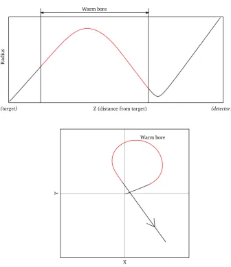
Figure 2.1: Z-R and X-Y views of a typical ion path through the solenoid.
since it is only a 2D calculation, it does not take into account the azimuthal variation in the field caused by the discrete components of the yoke, or the larger gap between the staves at the top or bottom of the solenoid. It is assumed that this has a negligible effect on the ion trajectories.
A typical ion path is shown in figure 2.1. There are three distinct segments to the path. The first is the portion from the target until it reaches the warm bore. The small fringing field here has only a minor effect on the ion, and so the trajectory is essentially a straight line. Once inside the warm bore, the focusing action of the solenoid is apparent in the Z-R view. The X-Y view (where the warm bore portion of the path is highlighted in red) shows the spiral path that causes this focusing. Finally, once the ion reaches the end of the warm bore, there again is little field to affect it and the trajectory becomes straight again. The focal point is relatively clearly defined by the minimum in the Z-R plot.
2.1.2 Magnetic field file
• The first column contains the radial distance, in centimeters.
• The second column contains the longitudinal distance through the solenoid, from an arbitrary point, in centimeters. The currently used magnetic field file used the centre of the coils as the “zero” point, though there is no requirement that this is the case.
• The next column contains the radial component of the magnetic field, in Gauss.
• The final column contains the longitudinal component of the magnetic field, also in Gauss.
While the units specified for the magnetic field are Gauss, Solirte does internal normalization of the values to obtain the requested magnetic field value – a magnetic field of 6.5 Tesla means that the magnetic field data will be normalized such that the maximum z-axis component of the magnetic field along the z axis (ie: down the centre of the solenoid) is exactly 6.5 Tesla.
The field can also be shifted along the z axis, though this is primarily used for checking the sensitivity of the measurements to the absolute position of the coils.
2.2
Gas interactions
Without the presence of gas in the solenoid bore, the simulation of SOLITAIRE is almost trivial. For an ion with a particular initial position, velocity, and charge state, the final position on the detector merely requires tracing the progress of a charged particle through the non-uniform magnetic as described in section 2.1. When gas is introduced to the system, however, three more processes occur which greatly complicate matters. These three processes – scattering, charge exchange, and energy loss – are discussed next. Ionization of the beam particles is ecapsulated inside the handling of charge exchange, as there is no difference (from the beam particle perspective) between the electron becoming free or being captured by a gas atom or molecule. Ionization of the gas is assumed to be negligible, and all gas atoms or molecules are assumed to be uncharged.
2.2.1 Scattering
Scattering is the best understood of the gas interaction processes. For the sake of simplicity, it is assumed that the gas in monoatomic, at a sufficiently low pressure such that the ion is only interacting with a single gas molecule at any point in time2. This simplified process is still a very complex quantum
mechanical situation – there is little interaction force between the ion and the gas atom until the electron clouds overlap (since from a distance the gas atom is uncharged). However, a classical approach can produce a relatively accurate approximation.
The most classical approach is that of Rutherford scattering. Here, the gas and beam atoms are treated as simple point charges corresponding to their nuclear charge. This approximation is valid when energies are high enough that the bulk of the scattering interaction occurs well inside the innermost electron orbit. In the gold foil backscattering experiment from which this model was first proposed, this was very much the case: at the point of closest approach, the separation of the gold and helium nuclei was (in the large angle cases) around 27 fm. This compares to the radius of the first electron orbital in gold of nearly 53,000 fm. Additionally, the helium ions were fully stripped, eliminating the complex interaction of the two electron clouds.
2
While conceptually and mathematically clean, this approach does not accurately describe the types of interactions occurring in the bore of SOLITAIRE due to the relatively unstripped gas and beam particles. A more accurate model involves a screening function, the shape of which describes the effect of the electrons in cancelling out the nuclear charge. This is usually described as altering the electric potential between the two atoms from 1r (whereris the distance between the two nuclei) toS(r)1r where S(r) is the screening function.
These screening functions can be empirical or theoretically based. The theoretical based screening functions (for example, that of Salvat et. al. [9]) are typically based around Hartree-Fock calculations of the electron density, since the screening at any particular radius is (classically speaking) closely related to the charge within a particular radius. Empirical functions (such as the Ziegler-Biersack-Littmark, or ZBL, from [10]) typically build off the Thomas Fermi model of electron orbital densities, with some adjustment factors that vary based on the beam ion and the gas atom. A significant advantage of the empirical functions is their computational simplicity.
Scattering in Solirte is done through one of three methods. The first is simply Rutherford scattering. While this is quick, it is not especially accurate due to mentioned ignoring of the screening effect of the electrons.
The second method is that used by TRIM86 – the so-called MAGIC scattering routine. Apart from my translation from Fortran to C++, no changes were made. This routine starts from a fast approximation to the distance of closest approach, and then proceeds through several Newton-Raphson iterations to improve the result.
The final method is similar to that used by GEANT4. I develped an independent implementation in C++ using the algorithms described in [11]. While currently this simply uses the ZBL potential, and thus returns essentially identical results to the MAGIC routine, it is trivial to extend it to other potentials if a better one is identified. This is in contrast to the MAGIC routine where there are many derived constants and a specialised initial approximation used. Performance is similar between the TRIM and GEANT4 algorithms – while heavily dependent on the particles and gas presure, running Solirte with the GEANT4 algorithm would typically see an approximately 10% drop in performance.
2.2.2 Charge exchange
Charge exchange is a much more complicated process than scattering. When two atoms are in close proximity, there is a chance that one of the electrons will transfer from one atom to the other. For ions passing through a gas, the time that the ion is close to any particular gas atom is short – therefore, if an exchange event occurs, the two atoms become distant very quickly and the electron cannot be transferred back.
Early discussions about the process centered around the valence electron velocity[12]. In a classical view, consider an uncharged heavy atom (atomic numberZ) passing slowly through a cloud of uncharged helium atoms. The outer electron in He− would be traveling at a much higher speed than the Z-th electron in the beam atom. Therefore, the chance of the electron jumping from heavy ion to the helium is minimal due to the large difference in velocity. However, if the beam atom is moving at a sufficiently high speed, the net speed of the outer electron would match that required of the third electron in He−. In this case, the electron is capable of (comparatively) easily jumping between the two atoms.
of these two approaches are viable for rapid simulation of ion trajectories due to the large number of calculations required.
Given a large number of ions, and a large number of charge exchanging events, the collection of ions will form an equilibrium charge state distribution (ECSD). This ECSD is often Gaussian-shaped, though small variations due to electron shell effects are common. A number of different approximations exist for the mean and the width of the Gaussian, though some care has to be taken for highly stripped ions – since the mean will be close to the number of protons in the atom, it will predict a non-zero probability that the ion will have a charge greater than the number of protons in the atom, which is of course impossible.
The second approximation that is made is to disregard multiple-electron transfers, and assume that only a single electron is exchanged in each interaction. This works surprisingly well, since the multiple electron transfers usually can be compensated for simply by an increased single electron transfer cross-section. Consequently, a number of approximations ([15], [16]) have been developed for single electron capture cross-sections.
These two approximations (the ECSD, plus the capture cross sections) can be used to derive the electron loss cross-sections. Through this method, the effect of multiple electron transfers is nearly completely taken into account, since the most important feature – the proportion of time that the ion spends in a particular charge state – is correct, up to the approximations made by the assumption of a Gaussian distribution. The only time this approximation does not do so well is where an equilibrium is not reached. This is primarily for transmission of beam-like particles, where the mean free flight length between charge exchange interactions can often be in the order of the length of the solenoid. However, the exact transmission rate of these particles is not required, so the issue is not a significant one for the systems being considered.
The first step in this process is to calculate the single-electron loss cross-sections from the two given distributions. Given an equilibrium charge state distribution Dq, 0≤q≤Z, and a capture cross section
distributionσc,q, the loss cross sectionsσl,q must satisfy
σc,q+1Dq+1+σl,q−1Dq−1−(σc,q+σl,q)Dq= 0
Expressing this as a linear equation with respect toσl:
Dq−1σl,q−1−Dqσl,q =σc,qDq−σc,q+1Dq+1
The points at q= 0 and q =Z are defined by setting σc,0 =D−1 =σl,Z =DZ+1 = 0. By inspection of
several terms, it becomes clear that the solution is
σl,q =
σc,q+1Dq+1 Dq
This can be verified by substitution:
σc,q+1Dq+1+σl,q−1Dq−1−(σc,q+σl,q)Dq
=σc,q+1Dq+1+ σc,qDq
Dq−1
Dq−1−
σc,q+
σc,q+1Dq+1 Dq
Dq
=σc,q+1Dq+1+σc,qDq−σc,qDq−σc,q+1Dq+1
= 0
Consider two exponential distributions characterized by cross-sections σ1 and σ2, ie: with
(normal-ized) probability distribution functions P1(d1 =x) = σ1exp−σ1x and P2(d2 =x) = σ2exp−σ2x. The
combined exponential distribution P(d=x) is defined as the probability of either event 1 or event 2 occurring in distancex. So
P(d=x) =P1(d1 =x)P2(d2> x) +P2(d2=x)P1(d1 > x)
=σ1exp (−σ1x) Z ∞
x
σ2exp −σ2x0
dx0+σ2exp (−σ2x) Z ∞
x
σ1exp (−σ1x)
=σ1exp (−σ1x)
−exp −σ2x0 ∞
x +σ2exp (−σ2x)
−exp −σ1x0 ∞
x
=σ1exp (−σ1x) exp (−σ2x) +σ2exp (−σ2x) exp (−σ1x)
= (σ1+σ2) exp [−(σ1+σ2)x]
This is simply an exponential distribution with cross-section σ1+σ2. Additionally, the probability that
the event that occurs is event 1 is
P(event 1 at d=x) = P1(d1 =x)P2(d2 > x) P(d=x)
= σ11 exp (−σ1x) exp (−σ2x) (σ1+σ2) exp [−(σ1+σ2)x]
= σ1 σ1+σ2
Combining the electron capture and loss cross-sections gives a single exponential distribution with cross-section σq = σc,q +σl,q and the probability of an electron capture event Cq = σc,qσ+c,qσl,q. The
mean free path is simply the result of combining the cross-section and the molecular density of the gas: dq= (σqN)−1 whereN is the molecular density of the gas according to the ideal gas law.
2.2.3 Energy loss
As an ion travels through material, energy is dissipated. The rate at which it is dissipated is termed the stopping power of the material.
The stopping power can be broken into two quantities. The first, the nuclear stopping power, is closely related to scattering. When a scattering interaction occurs, the beam particle is deviated from its original path. By conservation of momentum, the particle it scatters off must recoil. Therefore, there is some transfer of energy from the beam particle to the particle it is scattering off. The nuclear stopping power is simply then the rate of collisions multiplied by the average energy lost in the collision. If scattering is treated as a discrete event, then the calculation of the energy loss for a scattering event with a centre-of-mass angleθCM is, from [17]:
∆E =E4∗M1∗M2 (M1+M2)2
sin2
1 2θCM
Where M1 and M2 are the masses of the two particles interacting, θCM is the centre-of-mass scattering
angle, andE is the initial lab-frame energy of the ion.
electronic stopping power is essentially zero, since the net charge visible to all but the closest-passing gas atoms is zero.
A first-order perturbation-theory approach, such as the Bethe stopping power formula, indicates a stopping power proportional to q2. Consequently, the electronic stopping power is closely related to the charge exchange process. After an electron is lost by the ion, the instantaneous stopping power of the gas increases. However, there is also clearly interaction in the other direction. As the ion slows, the electron capture and loss cross sections change. Therefore, for a general simulation, neither the stopping power nor the capture and loss cross sections can be treated as static over the entire trajectory of the ion.
As such, electronic stopping power is handled in a semi-microscopic continuous way in Solirte. There are a number of approximations that exist for calculating the electronic stopping power of atoms in various materials. Solirte uses a combined Lindhard-Scharff[18]/Bethe-Bloch approach (for low and high energy regions respectively), and applies the energy loss after each integration step. Since the integration step size is dominated by the distance between charge exchange or scattering interactions, the energy loss over a single step for most ions is surprisingly constant regardless of the mass or speed of the ion. In all cases studied so far, the energy loss per step has been well below 1%, so there is little chance of the discrete jumps in energy causing significant variation in the results.
2.2.4 Energy interpolation
As can be seen above, the interactions with the gas vary with the energy of the particle. Additionally, the energy of the particle varies as it proceeds through the gas due to the stopping power of the gas. For beam-like particles this energy loss is minimal in most cases, but for the slow and heavy ERs it can be up to 10% or more. This is on top of the energy spread of the particles coming out of the target (both from scattering and evaporation). Any windows installed at either end of the bore have a significant effect as well.
Consequently, in many cases a single set of capture and loss cross sections – or cached scattering information or stopping powers – is insufficient to accurately model the progress of the ion through the solenoid. To compensate for this, all the energy-dependent information is pre-calculated at a number of energies and linear interpolation is used to calculate the values between the points. The precalculation starts at the highest possible energy, and proceeds down to 1 MeV, changing the energy at most 10% in any one step. If a 10% step in energy results in a change in any of the properties of over 5%, the energy step is halved and the step re-tried.
Once the properties have been calculated at the required energies, each ion being tracked is assigned to the relevant “interpolation bin” (one of the ranges as calculated above). Instead of using a fixed value for cross-sections etc., the value is calculated from a linear interpolation each time it is required. The energy of the ion is updated each integration step, and if it has gone outside the range for the current bin the next bin is selected. Additionally, the velocity is only rescaled when the bin is changed. Since the magnitude of the velocity of the ion has little effect on the overall result, this does not cause significant issues.
2.2.5 Input parameters
specifying the basic properties of the gas (atomic number and mass, pressure, and temperature), the ECSD approximation to use, and additional tuning parameters.
As described above, the ECSD requires two values – the mean charge state, and the width of the distribution. The mean charge state is specified through a base approximation, combined with two adjustment factors. The base approximation can be selected from a number of different approximations:
• Betz et. al[19] based on 1070 MeV S, As, I and U ions.
• Dmitriev and Nikolaev[20] based on a number of ions through nitrogen.
• Oganessian[21].
• “Popeko” – This is the original function that came with the program SOLENO, of unknown origin.
• Solid – Mean charge state used for the distribution out of the target[2].
• Schiwietz and Grande[22].
• Finally, an explicitly given value for ¯q can be used.
The ¯qapprox from this approximation is then adjusted by two further parameters: a scaling factor
(qscale) and an offset (qoffset). The mean charge state ¯q actually used by the simulator is calculated as
¯
qapproxqscale+qoffset. However, in most cases onlyqscalewould be used, andqoffsetis primarily for historical
compatibility3. The ECSD width can also be specified through several ways:
• Betz[23].
• Dmitriev and Nikolaev[20].
• Dmitriev and Nikolaev as implemented in the precursor Fortran code Solimike (slightly different than given above).
• HWHM used for the distribution out of the target[2].
• Again, an explicitly value value for qHWHM can be specified.
Finally, there are two additional “tuning” parameters for the gas. The first is an adjustment of the maximum scattering impact parameter. As described in [11], decreasing the maximum allowed impact parameter will result in an increase in the average free flight distance between scattering events. In cases where the number of scattering interactions is high, this allows the simulation to run faster but with a slight decrease in accuracy. The second tuning parameter is an adjustment on the scattering cross-section of the gas. This is primarily used to determine the impact of gas scattering on the image size at the detector.
2.3
Initial ion properties
There are two main methods for generating the state of each ion that is simulated out of the target. The first is to provide a position, normalized velocity vector, and energy for each ion. This is done via TRIM output files. The second method is to have Solirte generate the initial ion states itself.
3
2.3.1 Beam profile
The spatial distribution of the particles leaving the target is entirely due to the shape of the beam striking the target. Due to the upstream focusing components, the beam reaching SOLITAIRE is not entirely symmetric. Typically, the beam would have a Gaussian profile, but with the width in one axis being approximately twice the width in the other axis. This is handled in Solirte by specifying the width of the Gaussians in the two directions. There can also be an offset specified.
There is nothing in the simulator that requires the initial position to be a particular shape, and several other distributions have been used to investigate specific results. For example, to investigate the scattering of beam particles off the Faraday cup, an initial position distribution of a ring was used at the lip of the Faraday cup.
2.3.2 Angular distribution
The initial angular distribution of the particles leaving the target is used to perform a number of different tasks within Solirte. Since the initial angle and initial energy are correlated to some degree, the initial angular and energy distributions do not operate in isolation. The initial energy distribution is sampled first to obtain the nominal particle energy, and this value is passed through when selecting the initial angle. The initial angle sampler then modifies (“derates”) this energy depending on the physics it is intended to be approximating. Actual simulation of the scattering process in the target is not simulated.
Initial angular distribution of ERs
The most straightforward task of Solirte is simply to simulate the transmission of ERs through the solenoid. In this case, an initial angular distribution closely matching that of the real distribution expected out of the back of the target is required. Most measured ER angular distribution are specified in terms of a single Gaussian, or as the sum of two Gaussians. This is due to the kinematics of evaporation and scattering, and is described in more detail in section 5. There, the alternative of a Gaussian plus a step-Gaussian (a Gaussian with a mean above zero, and that is fixed at the peak value for angles below the mean) is also mentioned. Solirte supports the Gaussian plus step-Gaussian form, and the former two cases (double- and single-Gaussians) are simply special cases of this.
Initial angular distribution of beam-like particles
The second common task is to simulate the transmission of the beam-like particles through the solenoid. These have a very different initial angular distribution to ERs which can be very complicated – consider the case of an identical beam and target, with the resulting Mott scattering. For the sake of simplicity, such issues are not considered by Solirte. Instead, a simple Rutherford scattering initial angle distribution is used.
These can be trivially found by solving the three conservation equations:
vi,1m1 =vf,1m1cos (θ) +vf,2m2cos (φ) (Conservation of x-axis linear momentum)
0 =vf,1m1sin (θ) +vf,2m2sin (φ) (Conservation of y-axis linear momentum) vi,21m1 =vf,21m1+vf,22m2 (Conservation of energy)
Solving these gives:
vf,1 vi,1
=
cos (θ)±qm2
REL−sin2(θ)
1 +mREL
where
mREL= m2 m1
For a typical configuration, where the atomic mass of the target is higher than that of the beam, the negative case corresponds to a beam particle backscattered from the target. Since such particles are of no relevance to the solenoid transmission, the final velocity is always taken to be the positive case.
This distribution is the one used when simulating the beam-like particles through the solenoid.
One complication arising from the use of a Rutherford initial angular distribution is handling the divergence as the angle goes to zero. While one option is to simply cut off the distribution at some small value, this results in the vast majority of ions simply being collected by the Faraday cup. To improve the efficiency, Solirte first (randomly) picks the starting position based off the beam profile. By using the position to calculate a lower bounding angle just inside the Faraday cup, most ions avoid the Faraday cup. This does, however, intoduce a slight bias into the results, since ions with a small radius will be over-represented in the ions entering the warm bore. In most cases this is not a significant issue, since the absolute transmission of beam-like particles is not essential, merely the solenoid configuration that minimizes the transmission.
It should be noted that this optimization is only done when the simulator is put into “beam-like particle” mode. When simulating ERs, the full angular distribution is sampled for each particle.
Other angular distributions
While there are no limitations on the initial angular distribution, the third most commonly used dis-tribution is a uniform angular distributon. This is used for building up the transmission matrices used for reconstructing the initial angular distributions (as discussed in section 5.5), and for visualising the transmission through the solenoid as a function of energy and initial angle.
2.3.3 Energy distribution
As mentioned, the energy distribution is closely related to the angular distribution. There are typically two distributions used for the inital energy.
The first is a fixed beam energy, which is then converted into the correct energy distribution at each angle (through the angular derating process mentioned above). This is the mode which is usually used when calculating transmission ratios through the solenoid.
The second distribution is simply a uniform distribution between two energies, with no angular derating applied. In this case, the angular distribution is also usually either uniform over some angular range, or fixed in value. This is the form used to visualize the way that transmission varies as a function of energy and initial angle.
2.4
Conclusion
Due to the microscopic approach taken in the simulation, there is a significant amount of computation required for each ion. As a result, doing these calculations quickly is of high importance if the simulator is to be frequently used. This is the focus of the following chapter.
Simulator optimization
There are cases where a large number of ions need to be simulated using Solirte – for example, the use explained later where the transmission of the solenoid as a function of initial angle needs to be evaluated. Even on a multi-core processor, many hours of simulating may be required. Execution time in Solirte is spent in one of several places, depending on the system being simulated.
The initialization and finalization steps for each ion are fairly minimal, consisting mostly of sampling various distributions for position, energy, etc. In all normal use cases, this makes up less than 1% of the total execution time. Between initialization and finalization, the ion is repeatedly processed, moving downstream with each step.
The step consists of four phases. First of all, a fourth order Runge-Kutta-Fehlburg iteration is made. This consists of a significant number of multiply-accumulate operations, as well as a number of samplings of the magnetic field. Each of these samplings is a bilinear interpolation operation. After this step is completed, and assuming it does not need to be repeated with a smaller step size, the ion is checked for interactions with the environment:
• Charge exchange operations are very fast. All that is involved is the sampling of a uniform random number and a comparison with the capture/loss threshold.
• Scattering is significantly slower than charge exchange. In fact, a single scattering operation typically takes slightly longer than an integration step due to the complex mathematics involved.
• Hit-testing against the geometrical obstructions is somewhere in between, though can be slow if there are a large number of obstructions present since the distance to every obstruction is evaluated. To mitigate this, hit testing is deferred when possible as described below.
Clearly, in systems where the solenoid is being run in gas-free mode, the total scattering and charge exchange times are zero. In these cases, it is typical that the integration step dominates the execution time. However, when simulating slow-moving ERs in 1 Torr of helium, this decreases to approximately 50% of the time. Despite the scattering stage taking longer than the integration stage, the scattering is not done every step, leading to a lower total processor time over the complete tracing of the ion.
compared to even the fastest CPUs. However, they are not suited to all problems due to their simplistic scheduling design. Due to the mentioned ion independence, and the floating-point-heavy workload, Solirte makes an excellent candidate for processing on a GPU.
3.0.1 GPU execution architecture
Processing on a GPU is quite different to processing on a traditional CPU. A complete discussion on GPU architecture would be lengthy and largely unnecessary. Only a brief outline of the points relevant to Solirte will be discussed.
The typical workload of a GPU is processing a particular sequence of instructions for a large number of data sources (pixels, vertices, etc). Their architecture reflects this. In a modern general-purpose CPU, there can be several identical instruction units, each of which operate independently. In a GPU, things are slightly different – execution units are grouped together, and all execute the same instruction simultaneously, though on different data streams. This has a particular effect in branching (where code is conditionally executed).
To introduce some terminology, consider the rasterization stage of rendering a single triangle to a framebuffer. For each pixel to be rendered, a thread is created. All of these threads execute the same sequence of instruction, called the shader. These threads are grouped together into warps (from weaving terminology). The warp is the fundamental unit of threading in the GPU. A warp is assigned to a particular GPU core, where it will execute until it completes. Each core has a large number of warps, which it alternates between in some fashion, executing one instruction across all threads of some warp, then another instruction across all threads of another warp. In NVidia’s G80 GPU, a warp contains 32 threads. In AMD’s R600 GPU a warp contains 64 threads.
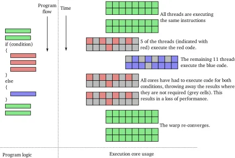
In a purely sequential shader with no branches, this presents no problem. All the threads of one warp execute in lock-step from start to end. The problem comes when branches are encountered. If all the threads of a warp take one direction in the branch, things continue unaltered. However, if both branch paths are taken, things become more complicated. Since a warp must execute the same instruction across all contained threads, it obviously cannot continue in this fashion if two of the threads are executing different instruction streams. As a result, the warp diverges – the one warp is changed into two warps, each containing a subset of the threads for a particular branch direction. These two warps then execute independently until they reach some other common point. This is shown diagrammatically in figure 3.1. A splitting of the execution paths is called a warp divergence, and the rejoining is called a warp convergence.
Clearly, a divergent warp has a large impact on the potential performance of the code. This becomes a problem when dealing with error-bounded loops, for example adaptive integration. A typical CPU implementation would, given a meta-timestep to integrate over, keep subdividing timesteps until the error limit is satisfied. For example:
ts = meta-timestep = given parameter erb = error bound = given parameter t = relative time = 0
stepsize = ts - t while (t < ts) {
if (condition) {
} else {
}
Program logic Execution core usage
All threads are executing the same instructions
5 of the threads (indicated with red) execute the red code.
The remaining 11 threads execute the blue code.
The warp re-converges.
All cores have had to execute code for both conditions, throwing away the results where they are not required (grey cells). This results in a loss of performance. Time
[image:43.595.73.533.255.564.2]Program flow
{
stepsize = smaller stepsize }
else {
stepsize = ts - t }
}
The problem with this code is that if any of the threads in the warp requires another loop in the while statement, all of the threads effectively take the loop. This means that the performance of all threads in a warp is determined by the performance of the worst thread in the warp. Clearly, this can have a severely detrimental effect on performance.
3.0.2 Integration of a time interval
The first step when integrating over the time interval to the next event is to determine the integration step size. This quantity must be small enough that any ion-obstruction intersections can be recorded and acted upon, and that the accuracy is good enough. It also must be large enough that excess time is not spent integrating very small step sizes that could be done using larger steps.
The traditional solution to this is to use an adaptive step size algorithm. In the system being integrated here, there is a problem: it is difficult, and computationally expensive, to accurately determine the distance the ion must travel before striking an obstruction. This is due to the complicated nature of the path of the ion through the solenoid. One option is to calculate the intersection point using the current position and velocity, and assuming the ion continues to travel in a straight line. This would be an “optimistic” way of predicting the distance, and would fail in cases where the ion would miss the obstruction with a straight line, but really hits due to the curved nature of the path. Furthermore, this hit could be missed if the ion passes completely through an obstruction in a single integration step.
A second option is to take the “pessimistic” approach and take the minimum distance between the current position and all points on the obstruction. In this case, the ion never (mathematically) hits the obstruction. Once it comes within a certain distance, it is regarded as having hit. The potential issue with this method is an ion traveling parallel to the face of the obstruction. In this situation, unnecessarily small timesteps would be taken. In the solenoid, this problem is lessened by the curved nature of the path, causing ions to eventually move away from an obstruction.
Once the stepsize is determined, the integration proceeds using the (4th/5th order adaptive) Runge-Kutta-Fehlberg method. After the integration step is done, any collisions, charge exchange, and scatter-ing events are handled.
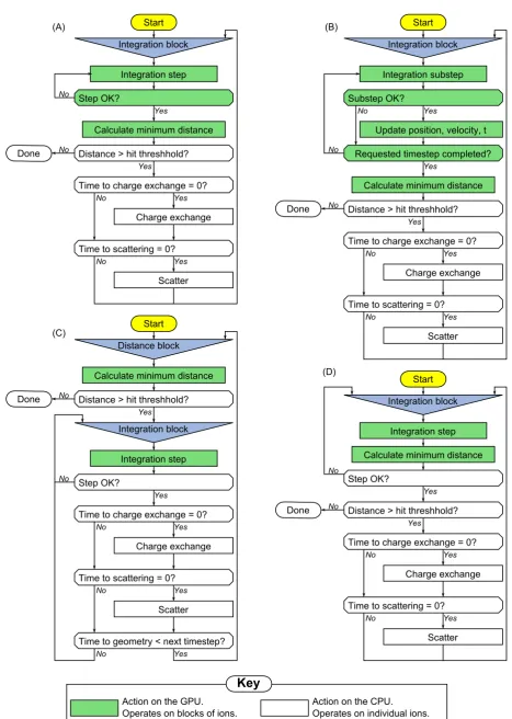
Four main integration architectures are shown in figure 3.2. The simplest architecture is shown in figure 3.2(a): the actual integration step and the distance to the closest obstruction are offloaded to the GPU. The GPU subdivides the requested integration step until the error condition is satisfied. The CPU then processes any events that need processing. While this uses the least bandwidth between the GPU and the system, it has the disadvantage as discussed before with the worst thread in a warp determining the performance.


![Figure 1.7: Primary decay modes for known nuclei (from NuDat2[6]).](https://thumb-us.123doks.com/thumbv2/123dok_us/1960303.156677/25.595.156.436.89.274/figure-primary-decay-modes-known-nuclei-nudat.webp)