Comparing the direct normal form and multiple scales methods through frequency detuning

through frequency detuning

.

White Rose Research Online URL for this paper:

http://eprints.whiterose.ac.uk/135000/

Version: Published Version

Article:

Elliott, A., Cammarano, A., Neild, S. et al. (2 more authors) (2018) Comparing the direct

normal form and multiple scales methods through frequency detuning. Nonlinear

Dynamics. ISSN 0924-090X

https://doi.org/10.1007/s11071-018-4534-1

© The Author(s) 2018. This article is distributed under the terms of the Creative Commons

Attribution 4.0 International License (http://creativecommons.org/licenses/by/4.0/), which

permits unrestricted use, distribution, and reproduction in any medium, provided you give

appropriate credit to the original author(s) and the source, provide a link to the Creative

Commons license, and indicate if changes were made.

[email protected] https://eprints.whiterose.ac.uk/

Reuse

This article is distributed under the terms of the Creative Commons Attribution (CC BY) licence. This licence allows you to distribute, remix, tweak, and build upon the work, even commercially, as long as you credit the authors for the original work. More information and the full terms of the licence here:

https://creativecommons.org/licenses/

Takedown

If you consider content in White Rose Research Online to be in breach of UK law, please notify us by

https://doi.org/10.1007/s11071-018-4534-1

O R I G I NA L PA P E R

Comparing the direct normal form and multiple scales

methods through frequency detuning

A. J. Elliott _· A. Cammarano _· S. A. Neild _· T. L. Hill · D. J. Wagg

Received: 3 August 2017 / Accepted: 22 August 2018 © The Author(s) 2018

Abstract Approximate analytical methods, such as the multiple scales (MS) and direct normal form (DNF) techniques, have been used extensively for investigat-ing nonlinear mechanical structures, due to their ability to offer insight into the system dynamics. A compar-ison of their accuracy has not previously been under-taken, so is addressed in this paper. This is achieved by computing the backbone curves of two systems: the single-degree-of-freedom Duffing oscillator and a non-symmetric, two-degree-of-freedom oscillator. The DNF method includes an inherent detuning, which can be physically interpreted as a series expansion about the natural frequencies of the underlying linear system and has previously been shown to increase its accuracy. In contrast, there is no such inbuilt detuning for MS, although one may be, and usually is, included. This paper investigates the use of the DNF detuning as the

Electronic supplementary material The online version of this article (https://doi.org/10.1007/s11071-018-4534-1) contains supplementary material, which is available to authorized users.

A. J. Elliott (

B

School of Engineering, University of Glasgow, Glasgow G12 8QQ, UK

e-mail: [email protected] S. A. Neild·T. L. Hill

Department of Mechanical Engineering, University of Bristol, Bristol BS8 1TR, UK

D. J. Wagg

Department of Mechanical Engineering, University of Sheffield, Sheffield S1 3JD, UK

chosen detuning in the MS method as a way of equat-ing the two techniques, demonstratequat-ing that the two can be made to give identical results up toε2order. For the examples considered here, the resulting predictions are more accurate than those provided by the standard MS technique. Wolfram Mathematica scripts implement-ing these methods have been provided to be used in conjunction with this paper to illustrate their practical-ity.

Keywords Nonlinear·Vibration·Normal form·

Multiple scales

1 Introduction

In recent years, there has been substantial interest in the study of backbone curves, due to their util-ity in studying lightly damped nonlinear vibrations in multi-degree-of-freedom (MDOF) mechanical struc-tures. The motivation for this paper comes from obser-vations made by the authors when comparing backbone curves found using the multiple scales (MS) method (see, for instance, [1]) and those found using the nor-mal form method, defined in [2].

particu-larly beneficial to the current work. We will call this the “direct” normal form (DNF) method1in order to dif-ferentiate it from the “classical” method described, for example, by Jezequel and Lamarque [4], Arnold [5], Murdock [6], Kahn and Zarmi [7] and Nayfeh [8]; the latter is not investigated here, as similar comparisons have previously been made, for example, in [2].

In recent years, the DNF method (and other nor-mal form methods similar to this) has been used exten-sively to capture the responses of nonlinear systems. This includes, but is not limited to, describing modal interactions and bifurcations in backbone curves [9– 12], recognising out-of-unison resonance in a taut cable [13], reduced-order modelling [14], nonlinear system identification [15,16], investigating aeroelas-tic systems under fluid flow [17,18], exploring appli-cability conditions for nonlinear superposition [19], and quantifying the significance of nonlinear normal modes [20]. In contrast with the recent development of the DNF method, the MS method is well established in the literature, with thorough discussions regarding its development readily available, for example, in [21– 26].

Perturbation methods require the repeated applica-tion of a number of steps, building up an increasingly accurate solution by addressing smaller terms in each repetition. In the practical application of these methods, the steps can require significant computational effort and produce increasingly complex expressions, which can, arguably, hide the mathematical insight gained from employing such a technique. In this paper, we consider the “accuracy” of these methods by assessing the result after one or two repetitions of their respective steps. It is generally recognised that these techniques converge to the correct solution with many repetitions, so can ultimately be considered as precise as each other. A contributing factor in the accuracy of the DNF method, as shown in [27], is the frequency detuning which arises in its formulation. In physical terms, this can be interpreted as a series expansion around the nat-ural frequency of the underlying linear system. This is not naturally present in the MS technique; however, several examples of alternative detunings, applied to MS technique, can be found in the literature [28–33]. The attempt that most closely resembles the detuning

1_{In some previous papers, this method is called “second-order}

normal form”, which is a phrase that is open to more than one possible meaning, so we choose to avoid it here.

of the DNF method is found in [32], although this pro-posed detuning is only employed in a small number of papers, such as [34,35]. In [32], anε-expansion is applied, not only to time, as is standard, but also to frequency. The paper presents the updated frequency– amplitude relationships and suggests that they appear more accurate, although it was not possible for this to be verified with numerical data. The motivation for expanding the frequency is solely to remove the secular terms in the response, and so the technique lacks the physical motivation that is present in the DNF method, as described in detail in the current paper.

Further attempts to detune the MS method have been proposed, though a number of these focus on the forced case in which it is common practice to perturb the forc-ing frequency [28,29]. A more thorough investigation is given in [30], and a comparison of the MS method and the generalised method of averaging can be found in [31]. Additionally, the detuning applied in [32] has also been applied to the Lindstedt–Poincaré method of strained parameters and the generalised method of aver-aging, with these detuned methods producing identical truncated results [33].

In this paper, a comparison on the DNF and MS tech-niques is provided, with emphasis placed on the detun-ing used. Specifically, in Sect.2, the two techniques are briefly outlined and compared using the Duffing oscil-lator as an example system, a system which is adopted in [27,31–33]. The two techniques are equated by intro-ducing a detuning step, which is physically interpreted as a perturbation about the response frequency rather than the linear frequency, into the MS technique in Sect.3. The detuning approach employed in the DNF method will be applied in the MS method, and it will be shown that doing so allows the two methods to be equated. By considering a more general detuning, it is shown that using MS both the fundamental and the har-monic response predictions are affected by the detun-ing. This is in contrast to the DNF technique, in which only the harmonic response changes. In Sect. 4, the techniques are compared for a two-mode system, where it is shown that the techniques give the same results if the MS method is modified to include the detuning. Conclusions are drawn in Sect.5.

2 Approximate methods

single-degree-of-freedom (SDOF) oscillator of the following form

¨

x+ω2_nx+εnx(x)=0. (1) Here, x denotes the displacement, ωn represents the linear natural frequency, andnx(x)is a nonlinear term. For both techniques, the nonlinear term is assumed to be small. Here, this is indicated byε, which may be thought of as a bookkeeping parameter that allows the relative size of terms to be tracked [8]. As such, εis taken to have a value of unity, such that it does not alter the equations. The application of the techniques is described as a series of steps, with the Duffing oscillator (nx(x)=αx3) being used as an example.

2.1 Direct normal form

The normal form approach is typically used to find peri-odic solutions to the equation of motion of a system. The objective of this approach is to apply a transform to the equation of motion to give a resonant form, in terms of transformed coordinateu, that can be solved exactly by using the following form for the solution, which assumes that system will respond as a single harmonic

u=up+um =

Ac 2 e

i(ωrt−φ0)₊ Ac 2 e

−i(ωrt−φ0)_{. (2)}

whereupandum are used to denote the positive and negative parts of the exponents, respectively, and Ac andωr represent the initial amplitude and nonlinear natural frequency, respectively. Time is denoted byt

andφ0denotes the phase of the response. Onceu has

been found, the harmonics of the response can be recov-ered using the transform equation.

The DNF approach is applied to equations of motion that are expressed in the linear modal coordinates,q, whereq = x for SDOF systems. This means that x

could be used instead ofq in the following equations. However,q has been kept to allow easier comparison with the MDOF case discussed in Sect.4. The trans-form may be summarised as

¨

q+ω2_nq+εnq(q)=0

q=u+εh1u1∗+ε2h2u∗2

−−−−−−−−−−−−−−−−−−→ ¨

u+(ω_r2+εδ)u+εnu1u∗1+ε2nu2u∗2=0.

(3)

Here,nq(q)represents the small nonlinear terms of the untransformed equation and, asq = x for a one

degree-of-freedom system,nq(q) = nx(q). In addi-tion, the detuningω2_n = ω_r2+εδ, which will later be utilised in the MS method, is applied. The harmon-ics are now captured by the product of h1, a 1×ℓ

vector of coefficients, andu∗₁, anℓ×1 vector consist-ing of all the combinations ofupandum that arise in

nq(up+um); these harmonics are also assumed to be small. The method of finding the harmonics,h1u∗1, and

the transformed nonlinear terms nu1u1∗ require three

steps. These are now discussed, along with their appli-cation to the Duffing oscillator. An explanation of how both the steps and the detuning are derived is given in Appendix A, together with an indication of how they may be modified for MDOF systems.

By eliminatingqfrom the original differential equa-tion in Eq. (3) using the transform and then simplifying using the transformed equation of motion, theεi bal-ance equation is given by the homological equation:

εi : −hiu¨∗i −ω2rhiui∗=neiu∗i −nuiu∗i. (4) The excitationof these equations, which defines the vectorsu∗_i, is given as

ε1: ne1u∗1=nq(u), (5) ε2: ne2u∗2=δh1u∗1+D{nq(u)}h1u1∗, (6)

where D{nq(u)}represents the Jacobian ofnq(u)and arises from the Taylor expansion ofn(q) = n(u +

εh1u∗₁ +ε2h2u∗₂). These equations are solved using

the following steps (which can be followed in Online Resource 1), first for the ε1 equation, as illustrated below, and then for theε2 terms by making the nec-essary modification to the first step.

Step1N FThe substitutionq =u =up+umis made in the nonlinear term to givenq(q)=nq(up+um)=

ne1u∗₁. Here,ne1contains coefficient values andu∗₁is

defined above.

For the Duffing oscillator,nq(up+um)=α(up+

um)3, giving

nq(up+um)=ne1u1∗=

α 3α 3α α ⎡

⎢ ⎢ ⎢ ⎣

u3_p u2_pum

upu2m

u3_m

⎤

⎥ ⎥ ⎥ ⎦ .

(7)

Step2N F Using Eq. (2), the variables up andum in

respect to time. The second derivative with respect to time can be expressed as a Hadamard product (◦); d2u∗₁/dt2= −dd◦u∗₁. Further details on this are given in Appendix A.

For the Duffing example, using Eqs. (2) and (7),u∗₁

may be written as

u∗₁=

⎡

⎢ ⎢ ⎣

u3_p u2_pum

upu2m

u3_m

⎤ ⎥ ⎥ ⎦ = A 3 c 8 ⎡ ⎢ ⎢ ⎣

ei3(ωrt−φ0) ei(ωrt−φ0) e−i(ωrt−φ0) e−i3(ωrt−φ0)

⎤ ⎥ ⎥ ⎦ , (8) and so

d2u∗₁

dt2 = −dd◦u

∗

1, where dd=ω 2

r

9 1 1 9⊺ .

(9)

Step3N F Now,h1andnu1may be found using

(dd⊺_−ω2

r11,ℓ)◦h1=ne1−nu1, (10)

where11,ℓ is a 1×ℓrow vector with every element

being one. This expression is derived in Eq. (A.7) in Appendix A. For each nonzero element in the brack-eted term, the corresponding value innu1is set to zero

and the value inh1is selected to satisfy the equation.

For the zero elements in the bracketed term, the corre-sponding terms innu1are set to match those inne1and

theh1terms are set to zero. The result of this is a series

of coefficients representing resonant terms innu1and

harmonic (i.e. non-resonant) terms inh1.

For the Duffing oscillator, Eq. (10) becomes

ω2_r

8 0 0 8

◦h1=

α 3α 3α α

−nu1.

(11)

This allows us to find the required vectors

h1=

_α

8ω2

r

0 0 α

8ω2

r

, nu1=

0 3α 3α 0

.

(12)

Note that the zeros on the left-hand side of Eq. (11) correspond to the resonant terms in Eq. (7) being set to zero, a feature that will also be observed in the MS method. Furthermore, it is important to note that there is some freedom of choice between the h1 and nu1

coefficients in Eq. (11). However, one of the advantages of this method is that the non-resonant terms, and only the non-resonant terms, inu∗ are removed from the transformed equation of motion.

The near-identity transform to orderε1may now be written as

q =u+εh1u∗1

= Ac

2 (e

i(ωrt−φ0)_+e−i(ωrt−φ0)₎

+ε _α

8ω_r2 0 0 α 8ω_r2

u∗₁

=Accos(ωrt−φ0)

+ε α 32ω2

r

A3_ccos(3(ωrt−φ0)).

(13)

From Eq. (3), along with Eq. (12), the transformed equation of motion may be written as

¨

u+ω_n2u+ε3αu2_pum+upu2m

=0. (14) To get the frequency–amplitude relationship for the backbone curve, we substitute the base solutions forup andum into Eq. (14) and then exactly balance either the ei(ωrt−φ0) _{or e}−i(ωrt−φ0) _{terms (there are no} non-resonant terms as these have been removed) to give

ωr =

ω2

n+ε 3α

4 A

2

c. (15)

This solution can be refined by repeating these steps, addressing the terms with increasing powers of εin turn. While each repetition leads to a more refined solu-tion, they becoming increasingly onerous to perform algebraically. Thus, it is desirable to approach the true solution in the smallest possible number of iterations. This basis will be used to compare the DNF and MS methods in later in the paper.

To illustrate this refinement, if the ε2 terms are included in the near-identity transform by repeating the steps a second time, the following, more precise, solution can be obtained:

q = Accos(ωrt−φ0)

+ε α 32ω2

r

A3_c

1+ε 3α 32ω2

r

A2_c

cos(3(ωrt−φ0))

+ε2 α

2

512ω4

r

A5_ccos(5(ωrt−φ0)). (16)

As a result, the frequency–amplitude relationship will now be given by

ω_r2=ω_n2+ε3α

4 A

2

c+ε2 3α2 128ω2

r

A4_c. (17)

2.2 Multiple scales

example, see [22,23,26,31,32] and references therein), and here we provide a brief summary of this technique to form a basis on which modifications can be discussed later.

Following this review of the method, in Sect.2.3, solutions found using the frequency detuning proposed in [32] will be presented; a more thorough investigation is given in Sect.3, in which a comparison will be made between this detuning and that used in the DNF method. The approach builds on the standard perturbation method in which the response is split into a series of terms with reducing significance x = X0+εX1+

ε2X2+ · · ·. In MS, each of these time-dependent

com-ponents are treated as functions of multiple timescales. If these timescales are used, this response is assumed to be of the form

x(t)=X0(τ,T,Ts)+εX1(τ,T,Ts)

+ε2X2(τ,T,Ts)+ · · ·

(18)

Here, the prescribed timescales are fast time over which oscillations occur,τ =ωt, a slower time over which the amplitudes evolve,T =εt, and a timescale which is slower still, given byTs =ε2t. This definition ofτ, which incorporates frequency, is more typically associ-ated with the Lindstedt–Poincaré method, but is applied here to allow a simpler comparison with the DNF method. These times,τ,T, andTs, are treated as inde-pendent variables, such that derivatives with respect to

tcan be expressed

dx

dt =ω

∂x

∂τ +ε ∂x

∂T +ε

2∂x ∂Ts

,

d2x

dt2 =ω 2∂2x

∂τ2 +2ωε ∂2x

∂T∂τ +ε 2∂2x

∂T2 +2ω ∂2x

∂Ts∂τ

.

(19)

Note that fast time–frequency,ωis typically set to the linear natural frequencyωn, such thatτ =ωt =ωnt. It is this selection of fast time that is now considered, and which gives the result listed in Table1.

Substituting Eq. (19) into a general representation of an undamped, unforced nonlinear oscillator and using ω=ωn, gives

¨

x+ω2_nx+εnx(x)=0

x =x(τ, T)

−−−−−−−−−→

ω2_nx††+ε2ωnx†‡+ε2(x‡‡+2ωnx†∗)

+ω2_nx+εnx(x)=0,

(20)

where•†= ∂•_∂τ,•‡= _∂∂•_T, and•∗= _∂∂•_T

s. Now,

substi-tuting Eq. (18) into the right-hand equation in Eq. (20),

removing the terms of orderε3and higher, and balanc-ing forεlead to

ε0:ω_n2X††₀ +ω_n2X0=0,

ε1:ω_n2X††₁ +ω_n2X1= −2ωnX₀†‡−nx(X0),

ε2:ω_n2X††₂ +ω_n2X2= −2ωnX1†‡−X ‡‡

0 −2ωnX†0∗

−D{nx(X0)}X1.

(21)

To find the solution for the components ofx, firstly the ε0order balance in Eq. (21) is solved to give

X0=A(T,Ts)cos(τ+φ (T,Ts)), (22) where A(T,Ts) and φ (T,Ts)are slow time-varying amplitude and phase functions, respectively, which are defined by the initial conditions of the system. This allows theε1equation of Eq. (21) to be written as

ω2_nX₁††+ω2_nX1=2ωnA(T,Ts)‡sin(τ+φ (T,Ts))

+2ωnA(T,Ts)φ (T,Ts)‡cos(τ +φ (T,Ts))

−nx(X0).

(23)

From Eq. (23), A(T,Ts), φ (T,Ts), and X1 may be

calculated using the following steps (as demonstrated in Online Resource 2), written atε1order. These steps may then be reapplied to theε2balance in Eq. (21), to find theε2solution.

Step1M SThe resonant terms, i.e. those that respond at τ = ωnt in Eq. (23), are removed and equated, writing

2ωnA(T,Ts)‡sin(τ+φ (T,Ts))

+2ωnA(T,Ts)φ (T,Ts)‡cos(τ +φ (T,Ts))

=Res{nx(X0)},

whereRes{nx(X0)}represents the resonant terms in

nx(X0).This equation is then solved to find A(T,Ts)

andφ (T,Ts).

For the Duffing oscillator example, we can write

2ωnA(T,Ts)‡sin(τ+φ (T,Ts))

+2ωnA(T,Ts)φ (T,Ts)‡cos(τ+φ (T,Ts))

=ResαA(T,Ts)3cos3(τ+φ (T,Ts))

= 3α

4 A(T,Ts)

3

cos(τ+φ (T,Ts)).

(24)

Balancing the sin(τ+φ)and cos(τ+φ)terms gives

A(T,Ts)‡=0, and

2ωnA(T,Ts)φ (T,Ts)‡= 3α

4 A(T,Ts)

respectively. These can be solved to give

A(T,Ts)=Ac(Ts),

φ (T,Ts)= 3α 8ωn

Ac(Ts)2T +φc(Ts),

(26)

whereφcis an integration constant representing a phase offset att=0. Hence, using Eq. (22), we can write

X0=Ac(Ts)cos(ωrt+φc(Ts)) ,

with: ωr =ωn+ε 3α 8ωn

Ac(Ts)2, (27)

where we have recalled thatτ =ωntandT =εtsuch thatτ+ε₈3_ωnα Ac(Ts)2T =ωrt.

Step2M SThe remaining terms in Eq. (23),

ω2_nX††₁ +ω_n2X1= −NRes{nx(X0)},

where NRes{nx(X0)} represents the non-resonant

terms in nx(X0)are now considered. Here the

right-hand side may be viewed as an “excitation” of a linear dynamic system in X1which can be solved to generate

harmonic responses terms in x.

For the Duffing oscillator example, we have

ω2_nX₁††+ω2_nX1= −NRes{nx(X0)}

= −α

4Ac(Ts)

3_cos(3(ω

rt+φc(Ts))) . (28)

where Eq. (27) has been used. Solving this linear dif-ferential equation gives

X1=

α 32ω2

n

Ac(Ts)3cos(3(ωrt+φc(Ts))) . (29)

Hence, the orderε1solution,x= X0+εX1, is given

by

x=Ac(Ts)cos(ωrt+φc)

+ α

32ω2

n

A3_ccos(3(ωrt+φc))

with: ωr =ωn+ε 3α 8ωn

A2_c.

(30)

Here, we have writtenAc(Ts)= Acandφc(Ts)=φc as the timescaleTsis not used to find theε1frequency– amplitude relationship.

As with the DNF methods, these steps can be repeated for higher-orderε terms. Applying these to theε2terms, the refined solution is given by

x=Accos(ωrt+φc)

+ε α 32ω2

n

A3_c1−ε 21α 32ω2

n

A2_ccos(3(ωrt+φc))

+ε2 α

2_A5

c 1024ω4

n

cos(5(ωrt+φc))

with: ωr =ωn+ε 3α 8ωn

A2_c−ε2 15α

2

256ω3

n

A4_c.

(31)

Again, Ac andφc are now a constants, though these would be functions of higher-order timescales if a higherε-order solution was being sought.

2.3 Duffing oscillator backbone curves

It is now possible to compare the expressions for the frequency–amplitude relationship derived using two repetitions of the steps in each method. These are given by

DNF:ω_r2=ω2_n+ε3α

4 A

2

c+ε2 3α2 128ω2

r

A4_c,

MS: ωr =ωn+ε 3α 8ωn

A2_c−ε2 15α

2

256ω3

n

A4_c.

(32)

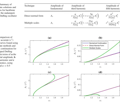
At this point, it is apparent that the DNF method detunes around the square of the response frequency, whereas the MS method directly detunesωr. The correspond-ing higher harmonic response amplitudes are given in Table1. Figure1 presents the fundamental and third harmonic backbone curves for the Duffing oscillator at ε1- andε2-order, along with the results found using the numerical continuation software Auto 07p [36]. In this figure, the influence that the type of detuning has on the results can be clearly seen. Both atε1- and atε2-order the DNF curve remains close to that of the numeri-cal solution, whereas the backbone derived from the MS method diverges from this at higher amplitudes. Considering panels (a) and (c), it is evident that theε2 -order solution remains close to the numerical curve for a greater range of amplitudes, though this introduces a hardening-to-softening behaviour at higher values of

A1. Further, the harmonic components are poorly

Table 1 Summary of approximate solutions and expressions for backbone curves for the undamped, unforced Duffing oscillator

Technique Amplitude of fundamental

Amplitude of third harmonic

Amplitude of fifth harmonic

Direct normal form Ac ε

α

32ω2

r

A3_c

1+ε 3α

32ω2

r

A2_c

ε2 α 2

512ω4

r

A5_c

Multiple scales Ac ε

α

32ω2

n

A3_c1−ε21α

32ω2

n

A2_c ε2 α

2

1024ω4

n

A5_c

Fig. 1 Comparison of first-order accurate (ε1₎

response curves found using approximate methods and numerical continuation for the undamped Duffing oscillator in terms ofathe fundamental amplitude,b the third harmonic andc other harmonics, using

ωn=1 andα=0.5

Numerical Continuation Direct Normal Form Multiple Scales (a₎

(c)

(b)

(d₎

MS relationship, the DNF method gives an implicit equation inω2_r. This can be easily rearranged to give a quadratic equation inω_r2which is easily solved and square rooted to give an explicit equation forωr. This process becomes more complicated at higher orders of ε, at which point it is possible that either a Taylor expan-sion or numerical continuation would need to be used. That being said, the accuracy of the curves in Fig.1 sug-gests that it is unlikely that these higher orders would be necessary to obtain a strong approximation of the true solution.

3 Equating the techniques

In this section, we compare the derivations of the DNF and MS approaches. To do this, we first consider fre-quency detuning. The importance of this step for the DNF method was assessed in [27], in which the Duffing oscillator was used to demonstrate that it is this

detun-ing which increases the accuracy of the technique in comparison with the classical normal form method. In light of the fact that perturbation methods repeat a spe-cific set of steps to find a solution, as demonstrated in Sect.2, we consider whether the same approach may be used in the MS method to improve the agreement with the DNF method at the same number of repetitions.

It should be noted that it is possible to introduce the intrinsic time-dependent amplitudes of the MS method to the DNF technique to allow transient behaviour to be captured. This is not investigated further here, as this paper focuses on the unforced, undamped behaviour of systems.

3.1 Detuning the MS method

the response frequency such that the substitutionω2_n=

ω_r2+εδcan be made, whereδis introduced as a detuning parameter. This is discussed in Appendix A where, for multiple degrees of freedom, the equation is written =Ŵ+εΔ. This allows the linear natural frequency to be replaced with the response frequency,ωr, and a detuning term,δ, in theε1relationship, Eq. (A.3), and results in coefficients in (dd⊺_−ω2

r11,ℓ) expression that

are exactly zero, seeSt ep3N F.

This detuning has been discussed in [37], where it was shown that the detuning does not affect the frequency–amplitude relationship, but does improve the prediction of the third harmonic. The physical inter-pretation of this is associated with how the underlying linear system is defined—normally we consider the Duffing oscillator to have a linear stiffness termω2_nx

(and hence a natural frequency of ωn), but the same result can be achieved by treating the linear stiffness term asω2_rxand modifying the nonlinear term to com-pensate for this, givingαx3+δx, whereδis a detuning parameter. Adopting the second approach can result in a smaller nonlinear term which more closely meets the key assumption that the non-linearity is of order ε1. Note that this interpretation of the detuning does not specifically rely on the assumption thatδis small, pro-vided the new nonlinear term,αx3+δx, remains small.

3.2 Detuned multiple scales

Now let us consider how frequency detuning, which we will view as a means to express the equation of motion in terms ofωr, may be used in a MS approach, resulting in thedetuned multiple scales approach(dMS). Firstly, when selecting the timescales we set the fast time as ω=ωr and henceτ =ωrt. The result of this is that Eq. (20) is modified to

¨

x+ω2_nx+εnx(x)=0

x =x(τ, T)

−−−−−−−−−→

ω_r2x††+ε2ωrx†‡+ε2x‡‡+ω2nx+εnx(x)=0, (33) where, now,τ =ωrt, whereas previously, in Eq. (21), τ =ωnt.

Now, we apply a frequency tuning to remove theωn terms. This tuning can take a number of forms, but let us select the same detuning as used in the DNF approach, with its link to modifying the linear and nonlinear stiff-ness terms, and useω2_n = ω_r2+εδ. Substituting this and Eq. (18) into Eq. (33) and balancing forεi give

ε0:ω_r2X††₀ +ω2_rX0=0,

ε1:ω_r2X††₁ +ω2_rX1= −δX0−2ωrX₀†‡−nx(X0),

(34)

which may be compared with Eq. (21) for the standard MS approach.

The solution to theε0equation is the same as before, namely Eq. (22), although note that now τ = ωrt, whereas, previously, τ = ωnt. The ε1 equation may be solved using the steps outlined previously.St ep1M S involves balancing the resonant term using the modified equation

−δA(T)cos(τ+φ (T))

+ 2ωrA(T)‡sin(τ+φ (T))

+ 2ωrA(T)φ (T)‡cos(τ+φ (T))=Res{nx(X0)},

(35)

and for the Duffing oscillator this results in

A(T)‡=0,−δA(T)+2ωrA(T)φ (T)‡

−3α

4 A(T)

3_=0. (36)

These can be solved to give

A(T)=constant=Ac, φ (T)=φc, δ= − 3α

4 A

2

c.

(37)

Note here, that the frequency shift is captured using δ, as δ is defined as the detuning parameter, and so φ (T)is set to a constant. Using this and recalling that ω2_n=ω_r2+εδresult in a frequency response equation given by

ωr =

ω2

n+ε 3α

4 A

2

c. (38)

This is identical to the expression obtained by the DNF, as shown in Eq. (15) and Table1.

Now,Step2M Sis applied to find the harmonics cap-tured byX1. With the resonant terms removed, theε1

balance may be expressed as

ω2_rX₁††+ω2_rX1= −NRes{nx(X0)}

= −α

4A

3

ccos(3(ωrt+φc)) , (39)

where X0 = Accos(τ +φc)andτ = ωrt has been used. Solving this differential equation gives

X1=

α 32ω2

r

Hence the orderε1solution,x = X0+εX1, is given

by

x =Accos(ωrt+φc)+ α 32ω2

r

A3_ccos(3(ωrt+φc))

with: ω2_r =ω_n2+3α

4 A

2

c. (41)

This is identical to the response predicted using the DNF approach, see Table1.

As previously mentioned, a similar detuning of the MS technique is considered in [32], which introduces anεperturbation,ω2 = ω2₀+εω1+ε2ω2+ · · ·, to

resolve the issues of secular terms in the response.2 Once truncated to orderε1, this expansion can be seen to be the same as that in the DNF method, though without the physical interpretation of a series expansion about the underlying natural frequency. It should be noted that, in [32], the first term is given as a square simply because it is convenient.

Note that the steps for the dMS method are illustrated in Online Resource 3.

3.3 Comparison of detuned multiple scales and direct normal form

It has been shown that the predicted response using the DNF method can be matched by the dMS method. Now we compare these two techniques in more detail for the case where the amplitude of response is assumed to be fixed, i.e. A(T)= Ac. As with all the discussions up to this point, we will consider theε1accuracy case for a SDOF system.

The form of the response for the methods may be written as

dMS: x =X0+εX1

DNF: x=q =u+εh1u1∗,

(42)

where theε0term on the right-hand side of both equa-tions represents the resonant response and theε1term the harmonic response. The resonant response takes the form

dMS: X0=Accos(τ+φc), τ=ωrt

DNF: u= Ac

2 e

i(ωrt−φc)₊ Ac 2 e

−i(ωrt−φc)

=Accos(ωrt+φc).

2_{Interestingly, it can be seen thatω}

0=ωn, even though theωi

terms are arbitrary in [32].

Here we have setφ (T)=φc as discussed in the pre-vious section. In both cases, the expression for the response frequency is derived by considering the reso-nant terms in theε1equation.

For MS, for the case whereA(T)=Acandφ (T)= φc, Eq. (35) can be simplified to give

−δAccos(ωrt+φc)=Res{nx(Accos(ωrt+φc))}, (43)

and hence, applying this in the dMS method and using ω2_n=ω_r2+εδ, we get

ω2_r =ω2_n+ 1

Accos(ωrt+φc) Res{nx(Accos(ωrt+φc))}.

(44)

In the case of the DNF approach, the transformed dynamic equation isu¨ +ω2_nu +εnu1u∗1 = 0 where

nu1u∗₁is determined usingSt ep3N F. This step solves (dd⊺ _{− ω}2

r11,ℓ) ◦ h1 = nq1 − nu1 by

consider-ing the elements term by term. For elements where (dd⊺_−ω2

r11,ℓ)=0, the resonant terms, the equation is

satisfied by setting the corresponding elements innu1

equal to those innq1. This is equivalent to stating that

nu1u∗₁ = Res{nqu∗₁} = Res{nq(q)}. By substituting this, along with the solution foruinto the transformed equation of motion and noting that, for a SDOF system,

nq=nx, we can write

−ω_r2+ω_n2Accos(ωrt+φc)

+Res{nx(Accos(ωrt+φc))} =0,

(45)

to obtain to the same expression as dMS, Eq. (43). Now, considering the harmonic contribution, from Eq. (39), we have

ω_r2X††₁ +ω_r2X1= −NRes{nx(X0)}. (46)

Recalling for the dMS technique that fast time is defined asτ =ωrt, the double derivative ofX1with

respect toτmay be written asX††₁ =(1/ω_r2)X¨1, hence

dMS: d

2

dt2{X1} +ω 2

rX1= −NRes{nx(X0)}. (47)

In the case of the DNF method, the harmonic terms are found inStep 3N Fwhere(dd⊺−ωr211,ℓ)◦h1=ne1−

nu1is considered. For the non-resonant, or harmonic,

elements this equation is satisfied by setting the left-hand side of the equation equal to the values inne1

in Appendix A, it can be seen that this solution arises from Eq. (A.3) and may be expressed as

−h1u¨∗1−Γh1u∗1=NRes{ne1u1∗} =NRes{nx(u)}. (48)

Recalling that, for a SDOF system,Γ =ω2_r and that

h1is a coefficient matrix, we can rewrite Eq. (48) as

DNF: d

2

dt2{h1u

∗

1} +ω2rh1u∗1= −NRes{nx(u)}. (49) It can be seen that this is the same as the harmonic expression for the direct MS approach, Eq. (46), by following the relationship in Eq. (42) and settingu =

X0andh1u∗1=X1.

From this, we can conclude that, at an accuracy level ofε1, the prediction of periodic oscillations using the DNF and MS methods can be made the same. This requires the MS technique to useτ = ωrt, as in the DNF method, for fast time and to removeωnfrom the equations of motion using the frequency tuningω_n2=

ω_r2+εδ. As discussed in [37], this is justified based on the idea that the system can be linearised about a stiffnessω_r2xrather thanω_n2xto potentially reduce the size of the nonlinear term. This may be substituted into Eq. (41) to give the full solution to orderε1.

3.4 Alternative frequency tunings

So far in this section, we have shown that the MS and DNF techniques are equivalent, to orderε1, under the special conditions that the fast time is set toτ =

ωrt and the stiffness term, ω2nx, in the equation of motion is rewritten as(ω2_r +εδ)x, whereδ can still be viewed as a detuning parameter. However, this fre-quency tuning approach raises the question about the predicted response when a different detuning parame-ter is selected.

For the case of the DNF method, this has been addressed in [37] for both single- and multi-degree-of-freedom systems. Consider the arbitrary frequency tun-ingω_n2=ω2_d+δd, whereωdis the detuned frequency withωd =ωr for the standard technique described in 2.1. In the MDOF notation used in Appendix A, the equivalent expression is=Ŵd+Δd. In [37], it was shown that the prediction of the response at the funda-mental frequency is independent of the chosen detuning at orderε1. The reason for this is that the only change to theε1balance, Eq. (A.3), is thatŴd, a diagonal matrix

ofω2_{r i} terms, is replaced by a diagonal matrix ofω2_di terms. The result is that, in St ep3N F,h1andnu1are

now found using Eq. (10).

When satisfying Eq. (10) using the arbitrary fre-quency tuning, we apply the rule defined inSt ep3N F to entries that are approximately zero in the brackets, rather than looking for values which are exactly zero. The corresponding terms innu1 are still set to those

innq1. As these terms are the same as those for the

case whereωd =ωr, the resulting nonlinear function inu,nu1, also remains the same. Hence, theε1order

equation of motion inu, and the subsequent response at the resonant frequency, is independent of the selection ofωd. However, the harmonic response prediction is affected, as each term in this is dependent on the non-near-zero value of the bracketed term in Eq. (10). The result is that, for the Duffing oscillator, the vector for

h1becomes

h1=

α

9ω2

r −ω2d

0 0 α

9ω2

r −ωd2

(50)

which may be compared to Eq. (12) for the case where the standard frequency tuning,ωd =ωr, is used. Thus, in contrast to the fundamental frequency response, which is not a function of the detuning parameter, the prediction for the third harmonic amplitude is depen-dent on the choice of detuning frequency and is given by

A3=

αA3_c

4(9ω2

r −ω2d)

. (51)

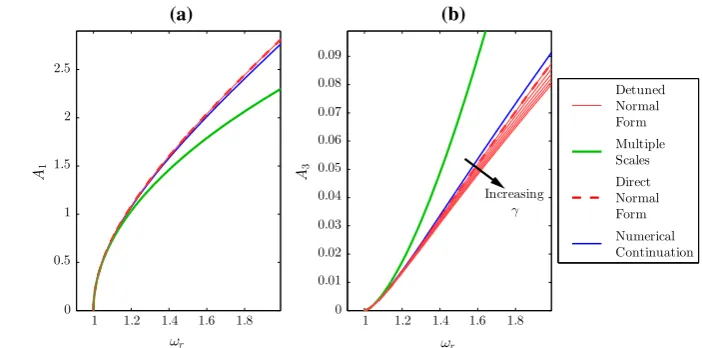
Figure2shows the DNF prediction of the response of the Duffing oscillator in terms of the first and third har-monics for a range of frequency tuning frequencies, ωd =ωr +(ωn−ωr)γ, fromγ =0, corresponding to the standard detuning used in DNF (i.e.ωd =ωr) toγ =1, where no detuning is used (i.e.ωd = ωn). Figure2a shows that the prediction of the response at the resonant frequency is robust to the choice of detun-ing parameter; however, the third harmonic response is affected by its choice and is better captured using the standard DNF detuning (γ =0) than with no detuning (γ =1).

Fig. 2 aFundamental and bthird harmonic amplitude response curves for the undamped Duffing oscillator, usingωn=1,

α=0.5, andγ ∈[0,1]

(a₎

ωr

A1

1 1.2 1.4 1.6 1.8 0

0.5 1 1.5 2 2.5

Increasing

γ

(b)

ωr

A3

1 1.2 1.4 1.6 1.8 0

0.01 0.02 0.03 0.04 0.05 0.06 0.07 0.08 0.09

Numerical Continuation Direct Normal Form Multiple Scales Detuned Normal Form

ε0:ω2_dX††₀ +ω_d2X0=0,

ε1:ω2_dX₁††+ω_d2X1=δdX0−2ωdX0†‡−nx(X0),

(52)

where the εiω2_nXi terms have been rewritten as εiω2_dXi +εi+1δdXi prior to the balancing using the ω2_n = ω2_d+δd frequency tuning expression. In addi-tion, the Taylor series expansionωn=ωd+εδd/(2ωd) has been used to removeωnin the slow dynamics term 2ωnX0†‡.

Following this approach results in X0 =

A(T)cos(τ+φ (t))= A(T)cos(ωdt+φ (t))and, using theε1equation, we find that, for the Duffing oscillator,

A(T)‡=0,−δdA(T)+2ωdA(T)φ (T)‡

−3α

4 A(T)

3_=0, (53)

which may be compared to Eqs. (25) and (36) for the MS and dMS techniques, respectively. Solving the dif-ferential equations inφ (T)andA(T)and substituting the solutions into theX0expression give

X0= A(T)cos(ωdt+φ (t))

= Accos

ωd+

δd 2ωd

+ 3α

8ωd

A2_c

t+φc

,(54)

where Acandφcare the values of A(T)andφ (T)at

t =0. Recalling thatδd is defined inωn2 =ω2d+δd, this gives the response frequencyωr = ωn2/(2ωd)+ ωd/2+3αA2c/(8ωd). Writingωd=ωr+(ωn−ωr)γ results in the response frequency equation

(1−γ2)ω_r2+(2ωnγ2)ωr

−

ω2_n(1+γ2)+3αAc

4

=0, (55)

and, from solving theε1expression, the resulting har-monic response amplitude is

A3=

αA3_c

32ω2_d =

αA3_c

32(ωr+γ (ωn−ωr))2

(56)

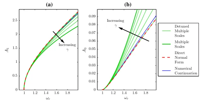
Figure3demonstrates that varyingγfrom 0 to 1 trans-forms the response from the DNF/dMS to the stan-dard MS response. For the MS technique,δd =0 and, hence, the frequency shift away formωnis captured by φ (T). However, for the dMS technique,ωd =ωr and soφ (T)=φcrepresents the fact that theX0response is

at response frequencyωr. These represent two special cases, for a general frequency tuning with fast time τ = ωdt; the thin, green curves in Fig. 3 represent a continuum between these two cases. Note that the accuracy of the DNF method is only reached when the detuning from that method is used. Interestingly, the fundamental response is independent of the detuning for the DNF method, whereas this is not the case for MS.

4 Example: non-symmetric, two-mass oscillator

A 2DOF system is considered in this section, allowing the two methods to be compared using a more com-plex system, as well as examining the robustness of the frequency tuning methods.

Fig. 3 aFundamental and bthird harmonic amplitude response curves for the undamped Duffing oscillator, usingωn=1,

α=0.5, andγ ∈[0,1]

ωr

A1

(a)

Increasing γ

1 1.2 1.4 1.6 1.8 0

0.5 1 1.5 2 2.5

ωr

A3

(b)

Increasing γ

1 1.2 1.4 1.6 1.8 0

0.01 0.02 0.03 0.04 0.05 0.06 0.07 0.08 0.09

Numerical Continuation Direct Normal Form Multiple Scales Detuned Multiple Scales

and one connecting the two masses. Therefore, the force-deflection equation for the grounding of the first mass is F =k1(Δx)+κ1(Δx)3and the relationship

is similar for the springs connecting the masses, given by F = k2(Δx)+κ2(Δx)3. Here,ki andκi are the spring constants of the linear and nonlinear springs, respectively. As in [38], both techniques are applied directly to the modal equations of motion to ease the comparison of solutions. These are given by

¨

q+q+Nq(q)=0 (57)

where is a diagonal matrix of the squared natural frequencies of the underlying linear system,ω2_ni, and

Nq(q)= κ1

2m

(q1+q2)3

(q1+q2)3+βq23

, (58)

withβ =16κ2

κ1.

The application of the methods is largely the same as for the Duffing oscillator considered in previous sections, so only a brief overview is given below. For brevity, solutions will only be considered to orderε1. In addition, we provide scripts, as supplementary mate-rial, that allow the equations to be derived symbolically using Wolfram Mathematica.

4.1 Multiple scales

Standard perturbations are again implemented, giving the two modal coordinates as

q1(t)=Q10(τ1, T)+εQ11(τ1, T)+ · · · ,

q2(t)=Q20(τ2, T)+εQ21(τ2, T)+ · · ·.

(59)

The notationτi =ωnit has been introduced to ensure that the fast time for each mode corresponds to the

appropriate natural frequency. It should be noted that, for this model, we consider the caseτ1≈τ2.

Implementing this perturbation, as well as the corre-sponding adaptation of the derivative given in Eq. (19), results in zeroth- and first-order perturbation equations that take the same form as in Eq. (21), and hence, the former can be solved to give

Q10= A1,1(T)cos(τ1+φ1(T)),

Q20= A2,1(T)cos(τ2+φ2(T)),

(60)

where Ai,j denotes the amplitude of the jth harmonic in theith mode. These solutions can be applied to the first-order equation [equivalent to the SDOF equation in Eq. (21)] to give theε1equations

ω2_n1Q††₁₁+ω2_n1Q11

=2ωn1A1,1(T)‡sin(τ1+φ1(T))

+A1,1(T)

8 (16ωn1φ

‡ 1(T)

−3κ1[A1,1(T)2+2A2,1(T)2])cos(τ1+φ1(T))

−nq1(Q10,Q20),

ω2_n2Q††₂₁+ω_n2₂Q21

=2ωn2A2,1(T)‡sin(τ2+φ2(T))

+A2,1(T)

8 (16ωn1φ

‡

2(T)−3κ1[A1,1(T) 2

+2(1+β)A2,1(T)2])cos(τ2+φ2(T))

−nq2(Q10,Q20). (61)

The nonlinear terms,nqi(Q10,Q20), are lengthy and

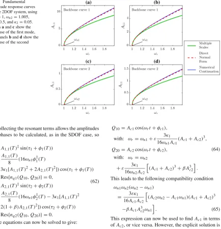
Fig. 4 Fundamental amplitude response curves for the 2DOF system, using

ωn1=1,ωn2=1.005, κ1=0.5, andκ2=0.05.

Panelsaandcshow the response of the first mode, and panelsbanddshow the response of the second mode

ωr

A1

,

1

ωn1 Backbone curve 1

(a₎

1 1.2 1.4 1.6 1.8 0

5 10

ωr

A2

,

1

ωn1 Backbone curve 1

(b)

1 1.2 1.4 1.6 1.8 0

2 4

ωr

A1

,

1

ωn2 Backbone curve 2

(c)

1 1.2 1.4 1.6 1.8 0

0.5 1

ωr

A2

,

1

ωn2 Backbone curve 2

(d)

1 1.2 1.4 1.6 1.8 0

0.5 1

1.5 Numerical

Continuation Direct Normal Form Multiple Scales

Collecting the resonant terms allows the amplitudes and phases to be calculated, as in the SDOF case, so that

2ωn1A1,1(T)‡sin(τ1+φ1(T))

+ A1,1(T)

8 (16ωn1φ

‡ 1(T)

−3κ1[A1,1(T)2+2A2,1(T)2])cos(τ1+φ1(T))

−Res{nq1(Q10,Q20)} =0,

2ωn2A2,1(T)‡sin(τ2+φ2(T))

+ A2,1(T)

8 (16ωn1φ

‡

2(T)−3κ1[A1,1(T)2

+2(1+β)A2,1(T)2])cos(τ2+φ2(T))

−Res{nq2(Q10,Q20)} =0.

(62)

These equations can now be solved to give:

A1,1(T)= Ac1,

φ1(T)=

3κ1

16ωn1Ac1

(Ac1+Ac2)3T +φc1,

A2,1(T)= Ac2,

φ2(T)=

3κ1

16ωn2Ac2

((Ac1+Ac2)3+βA3c2)T+φc2,

(63)

whereβ = 16κ2

κ1 . Note that the expressions for phase enforce the condition that neither fundamental ampli-tude can be equal to zero. Therefore, recalling that τ1=ωn1tresults in

Q10= Ac1cos(ωrt+φc1),

with: ωr =ωn1+ε

3κ1

16ωn1Ac1

(Ac1+Ac2)3,

Q20= Ac2cos(ωrt+φc2),

with: ωr =ωn2

+ε 3κ1 16ωn2Ac2

(Ac1+Ac2)3+βA3c2

.

(64)

This leads to the following compatibility condition

ωn1ωn2(ωn2−ωn1)

= 3εκ1

16Ac1Ac2

(Ac2ωn2−Ac1ωn1)(Ac1+Ac2)3

−βAc1A3c2ωn1

. (65)

This expression can now be used to find Ac1in terms

of Ac2, or vice versa. However, the explicit solution is

non-trivial and is not shown here.

The resulting backbone curves from Eq. (64) are given in Fig. 4 and discussed in Sect. 4.3. Due to the involved process required to find the harmonics, analytical solutions for these are not given, but have been derived using Wolfram Mathematica and solved numerically to allow comparison between the tech-niques; this is discussed in Sect.4.3.

4.2 Direct normal form

given. The resonant equations of motion are once again found in terms ofu, with

ui =ui p+ui m =

Aci 2 (e

+i(ωrt−φi)₊

e−i(ωrt−φi)). (66)

St eps1N F–3N F are followed as previously described and are not shown here due to the large size of the matrices involved. Full workings are shown in [38].

The frequency–amplitude relationships that arise are given by

3κ1(Ac1+Ac2)3

8m +Ac1(ω

2

n1−ω 2

r)=0, 3κ1[(Ac1+Ac2)3+βA3c2]

8m +Ac2(ω

2

n2−ω 2

r)=0. (67)

These results are comparable with Eq. (64) and the resulting backbone curves are, again, displayed in Fig.4. Similarly, the equations for the harmonics are algebraically complex and are solved numerically.

4.3 Detuned multiple scales

The key difference when applying the dMS in two degrees of freedom (2DOF) is that separate frequency tunings are to be applied to each mode

ω2_ni =ω_r2+εδi, fori =1,2. (68) Again, the resonant equations are used to find the ampli-tude, phase, and now detuning parameter. For the 2DOF case under consideration, these are given by

A1,1(T)=Ac1, φ1(T)=φc1,

δ1=

3κ1

8ωn1Ac1

(Ac1+Ac2)3,

A2,1(T)= Ac2, φ2(T)=φc2,

δ2=

3κ1

8ωn2Ac2

(Ac1+Ac2)3+βA3c2

.

(69)

Thus, substituting these values into Eq. (68) gives the frequency–amplitude equations as

3κ1(Ac1+Ac2)3

8m +Ac1

ω2_n1−ω_r2=0,

3κ1(Ac1+Ac2)3+βA3_c2

8m +Ac2

ω2_n2−ω_r2=0. (70)

Comparing these with Eq. (67) demonstrates that the results from the dMS method, once again, match those

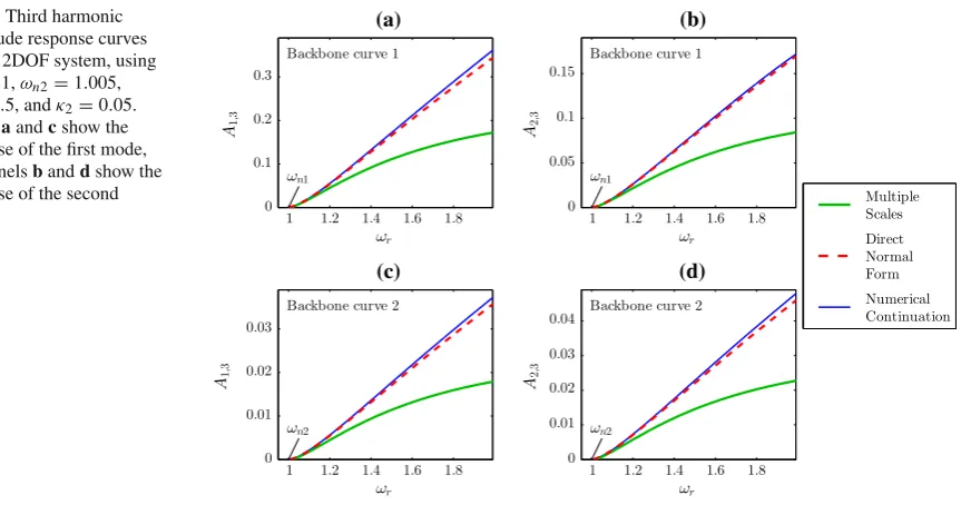
from DNF. It should be made clear that, in Figs.4and 5, the curve for the dMS method has not been printed as it is coincident with the DNF curve.

As with the SDOF case, the final forms ofqi are identical, though this is not shown here for reasons of brevity.

4.4 Comparison of the techniques

The fundamental backbone curves for the first and sec-ond modal responses are given in Fig.4. Four backbone curves are shown for each technique. Panels (a) and (b) correspond to the first backbone curve of the sys-tem, that is, the curve which initiates at the first natural frequency of the underlying linear system,ωn1;

pan-els (c) and (d) represent the second backbone curve. These results are comparable to those for the Duffing oscillator in Fig.1, with the MS curve underestimating the numerical continuation results and the DNF/dMS results again remain closer to the numerical continua-tion results. The difference between the methods grows significantly with increasing amplitude. In particular, the MS results diverge noticeably from the numerical and DNF/dMS counterparts at higher amplitudes. As verified in [38], this is the result of the loss of influence of the higher-order terms during the linearisation of the system.

Interestingly, the third harmonic components of the backbone curves in Fig. 5 are qualitatively different from the equivalent curve for the Duffing oscillator. While the amplitudes of the third harmonics from the MS method in the SDOF case were greater than those from numerical continuation, Fig. 5 shows that the opposite is true for the 2DOF responses. This incon-sistency suggests that the MS method is less robust to changes in the system compared to the DNF and dMS methods, which remains consistent across the two cases, although higher-order cases have not been con-sidered in this study.

5 Conclusions and discussion

Fig. 5 Third harmonic amplitude response curves for the 2DOF system, using

ωn1=1,ωn2=1.005, κ1=0.5, andκ2=0.05.

Panelsaandcshow the response of the first mode, and panelsbanddshow the response of the second mode

ωr

A1

,

3

(a₎

ωn1

Backbone curve 1

1 1.2 1.4 1.6 1.8 0

0.1 0.2 0.3

ωr

A2

,

3

(b)

ωn1

Backbone curve 1

1 1.2 1.4 1.6 1.8 0

0.05 0.1 0.15

ωr

A1

,

3

(c)

ωn2

Backbone curve 2

1 1.2 1.4 1.6 1.8 0

0.01 0.02 0.03

ωr

A2

,

3

(d)

ωn2

Backbone curve 2

1 1.2 1.4 1.6 1.8 0

0.01 0.02 0.03 0.04

Numerical Continuation Direct Normal Form Multiple Scales

whether a similar level of accuracy could be achieved. The frequency detuning, which can be physically inter-preted as a way of reducing the amplitude of the nonlin-ear term based on adapting the effective linnonlin-ear stiffness, is inherent in the DNF method and has been shown to improve the prediction of the harmonic response con-tent. In applying this detuning in the MS method, it was shown that the two methods could be equated, giving identical solutions up toε2order.

The DNF is advantageous insofar as a natural detun-ing approach is intrinsic in its formulation, whereas this is not the case for the MS technique. It is, therefore, the decision of the user as to whether a detuning is utilised to increase the accuracy of the method. Furthermore, it has been demonstrated that the fundamental response prediction is robust to changes in detuning in the DNF method. Since this is not the case for the MS technique, we observe that there is room for further optimisation of the detuning to be applied, which could further increase the accuracy of the method.

To aid the understanding of these methods, as well as the differences in their implementation, Wolfram Mathematica files for the 2DOF case have been pro-vided as open access data files. These closely follow the steps defined in Sect.2and are designed to be used in conjunction with this paper to give a practical under-standing of each procedure.

Acknowledgements S.A. Neild gratefully acknowledges sup-port from the EPSRC via the fellowship EP/K005375/1.

Open Access This article is distributed under the terms of the Creative Commons Attribution 4.0 International License (http:// creativecommons.org/licenses/by/4.0/), which permits unrest-ricted use, distribution, and reproduction in any medium, pro-vided you give appropriate credit to the original author(s) and the source, provide a link to the Creative Commons license, and indicate if changes were made.

Appendix A

Considering a MDOF system, expressed in linear modal coordinates, the direct normal form, to orderε accuracy, involves the transform

¨

q+Λq+εnq(q)=0

q=u+εh1u1∗

−−−−−−−−−−−→ ¨

u+Λu+εnu1u∗1=0.

(A.1)

Here,Λis a diagonal matrix with theithdiagonal ele-ment being the square of theithlinear natural frequency, ω2_ni. This reduces to Eq. (3) for the case where a single mode is considered, withq = q,u =u,n =n and Λ=ω2_n1=ω2_nto indicate that the terms are now scalar quantities or functions.

To find vectoru∗₁, we make use of the fact that in the transformed equation of motion the harmonic terms have been removed such that the response in the ith

coordinatesuimay be expressed as

ui =upi+umi

= Aci

2 e

i(ωr it−φ0i)₊ Aci

2 e

Using this the nonlinear functionnqexpressed in terms ofumay be written asnq(u)=nq(up+um)=ne1u∗1.

Hereu∗is anℓ×1 vector consisting of allℓ combi-nations ofupi andumigenerated bynq(up+um)and

ne1is an×ℓmatrix (for anndegree-of-freedom

sys-tem) that contains coefficient values. The subscripte

inne1indicates that this term can be thought of as an

excitationterm in the following discussion.

Now, considering Eq. (A.1), the transform can be substituted into the equation of motion inq. The result-ing expression can first be simplified usresult-ing the resonant equation of motion and then balanced in terms ofεto give

ε1:s−h1u¨∗₁−Γh1u₁∗=ne1u∗₁−nu1u∗₁, (A.3)

whereΓ is a diagonal matrix with theithdiagonal ele-ment being the square of theith response frequency, ω_{r i}2. Here, a Taylor series expansion has been used on the nonlinear function:n(q)=n(u)+O_{(ε). In} addi-tion, a form of frequency tuning, similar to that used in [37], is employed: we write Λ = Γ +εΔ when considering theh1u∗₁terms.

Now, observing that each element inu∗₁is made up ofupandumelements which themselves are complex exponentials in time, if follows that each term inu∗₁may be written as complex exponentials in time. Therefore, when differentiatingu∗twice with time, each element maps onto a scaled version of itself. So, we may repre-sentu¨∗₁as

d2u∗₁

dt2 = −dd◦u

∗

1 (A.4)

where dd is a vector of length ℓ×1 and ◦ is the Hadamard product (element-wise matrix multiplica-tion). Using this, we can write the first term in Eq. (A.3) as

−h1u¨∗1=h1dd◦u∗1

=

1n,1dd⊺◦h1u∗1,

(A.5)

where 1a,b is an a ×b matrix of ones. In addition, making use of the fact thatΓ is a diagonal matrix, the second term in Eq. (A.3) may be expressed in a similar form

Γh1u∗1=

Γ1n,ℓ◦h1u∗1. (A.6)

Substituting these into Eq. (A.3) gives

(1n,1dd⊺−Γ1n,ℓ)◦h1=ne1−nu1. (A.7)

It can be seen that this reduces to the equation given in

St ep3N Fof the normal form description for the SDOF

case (n = 1). Using St ep3N F, the equation can be solved to findh1andnu1and hence identify the

trans-form and transtrans-formed equation of motion, respectively.

References

1. Carbonara, W., Carboni, B., Quaranta, G.: Nonlinear nor-mal modes for damage detection. Meccanica51, 2629–2645 (2016)

2. Neild, S.A., Wagg, D.J.: Applying the method of normal forms to second-order nonlinear vibration problems. Proc. R. Soc. Lond. A467(2128), 1141–1163 (2011)

3. Touzé, C., Thomas, O., Chaigne, A.: Hardening/softening behaviour in non-linear oscillations of structural systems using non-linear normal modes. J. Sound Vib.273, 77–101 (2004)

4. Jezequel, L., Lamarque, C.H.: Analysis of nonlinear dynamic systems by the normal form theory. J. Sound Vib. 149(3), 429–459 (1991)

5. Arnold, V .I.: Geometrical Methods in the Theory of Ordi-nary Differential Equations. Springer, Berlin (1988) 6. Murdock, J.: Normal Forms and Unfoldings for Local

Dynamical Systems. Springer, Berlin (2002)

7. Kahn, P.B., Zarmi, Y.: Nonlinear Dynamics: Exploration Through Normal Forms. Dover Books on Physics. Dover, New York (2014)

8. Nayfeh, A .H.: Method of Normal Forms. Wiley, New York (1993)

9. Cammarano, A., Hill, T.L., Neild, S.A., Wagg, D.J.: Bifur-cations of backbone curves for systems of coupled nonlin-ear two mass oscillator. Nonlinnonlin-ear Dyn.77(1–2), 311–320 (2014)

10. Neild, S.A., Champneys, A.R., Wagg, D.J., Hill, T.L., Cam-marano, A.: The use of normal forms for analysing nonlinear mechanical vibrations. Philos. Trans. R. Soc. A373(2051), 20140404 (2015)

11. Lamarque, C.-H., Touzé, C., Thomas, : An upper bound for validity limits of asymptotic analytical approaches based on normal form theory. Nonlinear Dyn.70, 1931–1949 (2012) 12. Eugeni, M., Dowell, E.H., Mastroddi, F.: Post-buckling longterm dynamics of a forced nonlinear beam: a pertur-bation approach. J. Sound Vib.333, 2617–2631 (2014) 13. Hill, T.L., Cammarano, A., Neild, S.A., Wagg, D.J.:

Out-of-unison resonance in weakly nonlinear coupled oscillators. In: Proceedings of the Royal Society of London A: Mathe-matical, Physical and Engineering Sciences, vol. 471. The Royal Society

14. Touzé, C., Amabili, M.: Nonlinear normal modes for damped geometrically nonlinear systems: application to reduced-order modelling of harmonically forced structures. J. Sound Vib.298, 958–981 (2006)

15. Shaw, A.D., Hill, T.L., Neild, S.A., Friswell, M.I.: Periodic responses of a structure with 3:1 internal resonance. Mech. Syst. Signal Process.81, 19–34 (2016)