White Rose Research Online URL for this paper:
http://eprints.whiterose.ac.uk/103715/
Version: Accepted Version
Article:
Babaev, E, Carlstrom, J, Silaev, M et al. (1 more author) (2017) Type-1.5 superconductivity
in multicomponent systems. Physica C: Superconductivity and its Applications, 533. pp.
20-35. ISSN 0921-4534
https://doi.org/10.1016/j.physc.2016.08.003
© 2016 Elsevier B.V. This manuscript version is made available under the CC-BY-NC-ND
4.0 license http://creativecommons.org/licenses/by-nc-nd/4.0/
[email protected] https://eprints.whiterose.ac.uk/ Reuse
Unless indicated otherwise, fulltext items are protected by copyright with all rights reserved. The copyright exception in section 29 of the Copyright, Designs and Patents Act 1988 allows the making of a single copy solely for the purpose of non-commercial research or private study within the limits of fair dealing. The publisher or other rights-holder may allow further reproduction and re-use of this version - refer to the White Rose Research Online record for this item. Where records identify the publisher as the copyright holder, users can verify any specific terms of use on the publisher’s website.
Takedown
If you consider content in White Rose Research Online to be in breach of UK law, please notify us by
Type-1.5 superconductivity in multicomponent systems.
E. Babaev1, J. Carlstr¨om2, M. Silaev1 and J.M. Speight3 1Department of Theoretical Physics and Center for Quantum Materials,
The Royal Institute of Technology, Stockholm, SE-10691 Sweden
2 Department of Physics, University of Massachusetts Amherst, MA 01003 USA 3 School of Mathematics, University of Leeds, Leeds LS2 9JT, UK
In general a superconducting state breaks multiple symmetries and, therefore, is
charac-terized by several different coherence lengthsξi,i= 1, ..., N. Moreover in multiband material
even superconducting states that break only a single symmetry are nonetheless described,
under certain conditions by multi-component theories with multiple coherence lengths. As a
result of that there can appear a state where some coherence lengths are larger and some are
smaller than the magnetic field penetration lengthλ: ξ1≤ξ2... < √
2λ < ξM ≤...ξN. That
state was recently termed “type-1.5” superconductivity. This breakdown of type-1/type-2
dichotomy is rather generic near a phase transition between superconducting states with
different symmetries. The examples include the transitions betweenU(1) andU(1)×U(1)
states or betweenU(1) andU(1)×Z2 states. The later example is realized in systems that
feature transition between s-wave and s+is states. The extra fundamental length scales
have many physical consequences. In particular in these regimes vortices can attract one
another at long range but repel at shorter ranges. Such a system can form vortex clusters in
low magnetic fields. The vortex clustering in the type-1.5 regime gives rise to many physical
effects, ranging from macroscopic phase separation in domains of different broken
symme-tries, to unusual transport properties. Prepared for the proceedings of Vortex IX conference, Rhodes 12-17 September 2015.
I. INTRODUCTION
Below we briefly discuss the properties and occurrence of “type-1.5” superconducting state
characterized by multiple coherence length, some of which are smaller and some larger than the
magnetic field penetration length1 ξ1 ≤ξ2... < √
2λ < ξM ≤...ξN. Type-1 superconductors expel
weak magnetic fields, while strong fields give rise to formation of macroscopic phase separation in
the form of domains of Meissner and normal states.2,3The response of type-2 superconductors is the
following:4 below some critical valueH
c1, the field is expelled. Above this value a superconductor
forms a lattice or a liquid of vortices which carry magnetic flux through the system. Only at
a higher second critical value, Hc2 is superconductivity destroyed. These different responses are
the consequences of the form of the vortex interaction in these systems, the energy cost of a
boundary between superconducting and normal states and the thermodynamic stability of vortex
excitations. In a type-2 superconductor the energy cost of a boundary between the normal and the
superconducting state is negative, while the interaction between vortices is repulsive.4 This leads
to a formation of stable vortex lattices and liquids. In type-1 superconductors the situation is
the opposite; the vortex interaction is attractive (thus making them unstable against collapse into
one large “giant” vortex), while the boundary energy between normal and superconducting states
is positive. The ’ordinary’ Ginzburg-Landau model has a critical regime where vortices do not
interact.5,6 The critical value of κ in the most common GL model parameterization corresponds
to κ = 1/√2 (often the factor 1/√2 is absorbed into the definition of coherence length in which
case the critical coupling is κc = 1). The noninteracting regime, which is frequently called the
“Bogomolnyi limit” is a property of Ginzburg-Landau model where, at κc = 1/
√
2, the
core-core attractive interaction between vortices cancels at all distances the current-current repulsive
interaction5,6 (up to microscopic corrections beyond the standard Ginzburg-Landau theory). By
contrast in multi-component theories are characterized by multiple coherence length and do not in
general allow to form a single Ginzburg-Landau parameterκ.
The Ginzburg-Landau free energy functional for a multicomponent superconductor has the form
F = 1 2
X
i
(Dψi)(Dψi)∗+V(|ψi|) +
1
2(∇ ×A)
2, (1)
where ψi are complex superconducting components, D = ∇+ieA, and ψi = |ψi|eiθi, a = 1,2,
and V(|ψi|) stands for effective potential. We consider a general form of potential terms but the
simplest gradient terms. In general Eq.(1) indeed can contain mixed (with respect to components
ψi) gradient terms, e.g. Re[Dα=x,y,zψiDβ=x,y,zψj] (for a more detail on the effects of these terms
see7).
The multiple superconducting components can have various origins. First of all they can arise
in (i) superconducting states which break multiple symmetries. Such systems are described by
several order parameters in the sense of Landau theory of phase transitions, and have different
coherence lengths associated with them. Multiple broken symmetries are present even in the
simplest generalisation of the s-wave superconducting states: the s+is superconducting state,8,9
which breaks U(1)×Z2 symmetry.10 Likewise multiple broken symmetries are present in non-s
wave superconductors. Another example is mixtures of independently conserved condensates such
rich alloys.11,12Thereψi represents electronic and protonic Cooper pairs or deuteronic condensates.
A similar situation was discussed in certain models of nuclear superconductors in the interior of
neutron stars, whereψi represent protonic and Σ− hyperonic condensates.13,14
Another class of multi-component superconductors is(ii) systems which are described by
multi-component Ginzburg-Landau field theories that do not originate in multiple broken symmetries.
The most common examples are multiband superconductors.15–17 In this case ψi represent
su-perconducting components belonging to different bands. Since a priory there are no symmetry
constraints preventing interband Cooper pair tunnelling the theory contains generic terms which
describe intercomponent Josephson coupling η2(ψiψ∗j +ψiψ∗j). These terms explicitly break
sym-metry. Here the number of components ψi is not dictated by the broken symmetry pattern.
Multicomponent GL expansions can be justified when for example SU(N) or [U(1)]N symmetry
is softly explicitly broken down to U(1).18 Some generalizations of type-1.5 concepts for the case
of p-wave pairing in multiband systems was discussed in.19 Recently rigorous mathematical work
was done on justification of multicomponent Ginzburg-Landau expansions.20
A. Type-1.5 superconductivity
Multicomponent systems allow a type of superconductivity that is distinct from the type-1 and
type-2.1,7,10,18,21–25It emerges from the following circumstances: Multi-component GL models have
several fundamental scales, namely the magnetic field penetration depthλand multiple coherence
lengths (characteristic scales of the variations of the density fields) ξi, which renders the model
impossible to parametrize in terms of a single dimensionless parameter κ, thus making the
type-1/type-2 dichotomy insufficient for classifying and describing these systems. Rather, in a wide
range of parameters, there is a separate superconducting regime with some coherence lengths
that are larger and some that are smaller than the magnetic field penetration length ξ1/√2 <
ξ2/ √
2 < ... < λ < ξM/
√
2 < ... < ξN/
√
2. In that regime a situation is possible where vortices
have long-range attractive (due to “outer cores” overlap) and short-range repulsive interaction
(driven by current-current and electromagnetic interaction) and form vortex clusters coexisting
with domains of two-component Meissner state.1 The first experimental works24,25 put forward
that this state is realized in the two-band material MgB2. Moshchalkov et al termed this regime
“type-1.5 superconductivity”.24Recently experimental works proposed that this state is realised in
Sr2RuO426,27 and LaPt3Si.28,29 The experiments on the MgB2 were done using Bitter decoration,
done by cycling field and observing vortex cluster formation in different parts of the sample. In the
case of Sr2RuO4 the evidence of intrinsic mechanism of vortex cluster formation comes from µSR
experiment that observed vortex clusters contraction with decreasing temperature well below Tc
thus signaling attractive inter vortex forces rather than pinning responsible for clusterization. The
attractive inter vortex forces also provides and explanation for earlier experiment on Sr2RuO430
that reported vanishing creep in the absence of dramatic increase of critical current [initially in30
this was attributed to effects of domain walls trapping vortices. However such configurations
would have very characteristic magnetic signatures,31,32 these signatures were not observed in
surface probes26]. A prediction of a (narrow) region of type-1.5 state was made for certain interface
superconductors.33Also it was pointed out that a generic type-1.5 regime should form in iron-based
superconductors near transitions fromstos+ispairing states.10 Type-1.5 superconductivity was
discussed in the context of the quantum Hall effect34 and neutron stars.35 For other recent works
on this and related subjects see e.g..19,36–45
In these systems one cannot straightforwardly use the usual one-dimensional argument
con-cerning the energy of superconductor-to-normal state boundary to classify the magnetic response.
First of all, the energy per vortex in such a case depends on whether a vortex is placed in a cluster
or not. Formation of a single isolated vortex might be energetically unfavorable, while formation
of vortex clusters can be favorable, because in a cluster (where vortices are placed in a minimum of
the interaction potential), the energy per flux quantum is smaller than that for an isolated vortex.
Besides the energy of a vortex in a cluster, there appears an additional characteristic associated
with the energy of the boundary of a cluster. In other words for systems with inhomogeneous
vortex states there are many different interfaces, some of which have positive and some negative
free energy. The non-monotonic intervortex interaction is one of key properties of a type-1.5
su-perconductor, but is not a state-defining one. As discussed in the introduction and also below,
intervortex attraction can arise under certain circumstances in single-component materials as well.
In type-1.5 case this is a consequence of multiple coherence lengths and comes with a number of
new physical effects discussed below. We summarise the basic properties of type-1, type-2 and
single-component type-1 single-component type-2 multi-component Type-1.5 Characteristic
lengths scales
Penetration lengthλ&
coher-ence lengthξ (λ ξ <
1 √ 2)
Penetration lengthλ&
coher-ence lengthξ(λ ξ >
1 √
2)
Multiple characteristic density
variations length scales ξi, and
penetration length λ, the
non-monotonic vortex interaction
oc-curs in these systems in a large
range of parameters when ξ1 ≤
ξ2≤.... < √
2λ < ξM ≤...≤ξN
Intervortex in-teraction
Attractive Repulsive Attractive at long range and
re-pulsive at short range
Energy of su- perconduct-ing/normal state boundary
Positive Negative Under quite general conditions
negative energy of
superconduc-tor/normal interface inside a
vor-tex cluster but positive energy of
the vortex cluster’s boundary
The magnetic field required to form a vortex
Larger than the
thermo-dynamical critical magnetic
field
Smaller than
thermodynami-cal critithermodynami-cal magnetic field
In different cases either (i)
smaller than the
thermodynam-ical critthermodynam-ical magnetic field or (ii)
larger than critical magnetic field
for single vortex but smaller than
critical magnetic field for a
vor-tex cluster of a certain critical
size
Phases in ex-ternal magnetic field
(i) Meissner state at low
fields; (ii) Macroscopically
large normal domains at
ele-vated fields. First order phase
transition between
supercon-ducting (Meissner) and
nor-mal states
(i) Meissner state at low
fields, (ii) vortex
lat-tices/liquids at larger fields.
Second order phase
transi-tions between Meissner and
vortex states and between
vortex and normal states at
the level of mean-field theory.
(i) Meissner state at low fields
(ii) Macroscopic phase
separa-tion into vortex clusters
coexist-ing with Meissner domains at
in-termediate fields (iii) Vortex
lat-tices/liquids at larger fields.
Vor-tices form via a first order phase
transition. The transition from
vortex states to normal state is
second order.
Energy E(N) of N-quantum ax-ially symmetric vortex solutions
E(N) N <
E(N−1)
N−1 for all N.
Vor-tices collapse onto a single
N-quantum mega-vortex
E(N) N >
E(N−1)
N−1 for all N.
N-quantum vortex decays into
N infinitely separated
single-quantum vortices
There is a characteristic number
Nc such that E(NN) < E(NN−−11) for
N < Nc, while E(N)
N >
E(N−1) N−1
for N>Nc. N-quantum vortices
decay into vortex clusters.
TABLE I. Basic characteristics of bulk clean superconductors in type-1, type-2 and type-1.5 regimes. Here
the most common units are used in which the value of the GL parameter which separates type-1 and type-2
regimes in a single-component theory is κc = 1/ √
2. Magnetization curves in these regimes are shown on
H H
Hc Hc1 Hc Hc2
-M -M
H Hc
Hc1 Hc2
-M
Type-1 Type-2 Type-1.5
FIG. 1. A schematic picture of magnetization curves of type-1, type-2 and type-1.5 superconductors. The
magnetisation jump at Hc1 is one of the features of type-1.5 regime, however it is not a state-defining
property conversion of the Hc1 phase transition to a first order one can be caused by a number of
rea-sons (e.g. microscopic corrections near Bogomolnyi point, multi-layer structure, etc) in ordinary type-2
superconductors
II. THE TWO-BAND GINZBURG-LANDAU MODEL WITH ARBITRARY INTERBAND INTERACTIONS. DEFINITION OF THE COHERENCE LENGTHS AND
TYPE-1.5 REGIME
A. Free energy functional
Realization of the type-1.5 regime requires at least two superconducting components. In this
section we study the type-1.5 regime using the following two-component Ginzburg-Landau (TCGL)
free energy functional.
F = 1
2(Dψ1)(Dψ1) ∗+ 1
2(Dψ2)(Dψ2)
∗−νRen(Dψ
1)(Dψ2)∗ o
+1
2(∇ ×A) 2+F
p (2)
Here D=∇+ieA, and ψi =|ψi|eiθi,i= 1,2, represent two superconducting components. While
in general two components can have different critical temperatures, in the simplest case, the
two-band superconductor breaks only U(1) symmetry. Then eq. (2) can be obtained as an expansion
of the free energy in small gaps and small gradients.17,18,46–49 Such an expansion should not be
confused with the simplest expansion in a single small parameter τ = (1−T /Tc). The τ-based
expansion for U(1) system is an approximation that yields only one order parameter for a U(1)
system and neglects the second coherence length. The multi-parameter expansions that are not
based on symmetry are justified under certain conditions.18,49Indeed the existence of two bands in
a superconductor by itself is not a sufficient conditions for a superconductor to be described by a
of the theory (2) for two-bandU(1) systems see.18,22 Note that, in general in two-band expansion,
the terms corresponding to one component can be larger than a terms contributed by another
component. However as it will be clear below, for the discussion of typology of superconductors,
the relevant parameters are characteristic length scales associated with the exponential laws at
which field component restore their ground state values away from a perturbation such as a vortex
core (i.e. the coherence lengths). Indeed a component with smaller amplitude can give raise to a
longer coherence length that is important for intervortex interaction and should not be discarded
based merely on the smallness of amplitude |ψi|. In principle, for the component with larger
amplitude, one can keep higher-power terms in the GL expansion such as ψiψi∗(Dψi)(Dψi)∗,|ψi|6
etc. These terms lead to some corrections to two coherence lengths, while not affecting the overall
form of intervortex forces as can be seen from the analysis in.7 As be seen from the comparison
of vortex solutions in the GL formalism and in microscopic model without GL expansion,18 in the
regime of most interest these terms can be neglected.
We begin with the most general analysis by considering the case where Fp can contain an
arbitrarycollection of non-gradient terms, of arbitrary power in ψi representing various inter and
intra-band interactions. Below we show how three characteristic length scales are defined in this
two component model (two associated with density variations and the London magnetic field
penetration length).
The only vortex solutions of the model (2) which have finite energy per unit length are the
integerN-flux quantum vortices which have the following phase windings along a contourlaround
the vortex core: H
l∇θ1 = 2πN,
H
l∇θ2 = 2πN which can be denoted as (N,N). Vortices with
differing phase windings (N,M) carry a fractional multiple of the magnetic flux quantum and have
energy divergent with the system size,50 which under usual conditions makes them irrelevant for
the physics of magnetic response of a bulk system.
In what follows we investigate only the integer flux vortex solutions which are the energetically
cheapest objects to produce by means of an external field in a bulk superconductor. Note that
since this object is essentially a bound state of two vortices, it in general will have two different
III. COHERENCE LENGTHS AND INTERVORTEX FORCES AT LONG RANGE IN MULTI-BAND SUPERCONDUCTORS
In this section we give criterion for attractive or repulsive force between well separated vortices
in system (2) and condition for non-monotonic inter vortex forces following.1,7,21 We show how
it can be determined by analyzing Fp when ν = 0 and how three fundamental length scales are
defined in the model (2). If the model has mixed gradient terms they can be either treated as
in Ref.7 or eliminated by a linear transformation. By gauge invariance, Fp may depend only on
|ψ1|, |ψ2| and δ = θ1 −θ2. We consider the regime when Fp has a global minimum at some
point other than the one with |ψi| = 0, namely at (|ψ1|,|ψ2|, δ) = (u1, u2,0) where u1 > 0 and
u2 ≥0 (for discussion of phase-separated regimes see43). Then the model has a trivial solution,
ψ1 =u1,ψ2 =u2, A= 0, (i.e. the ground state). Here we are interested in models that support
axially-symmetric single-vortex solutions of the form
ψi =fi(r)eiθ, (A1, A2) = a(r)
r (−sinθ,cosθ) (3)
where f1, f2, a are real profile functions with boundary behavior fi(0) = a(0) = 0, fi(∞) =
ui, a(∞) = −1/e. No explicit expressions for fi, a are known, but, by analyzing the system of
differential equations they satisfy, one can construct asymptotic expansions for them at large r,
see.7,21
At large r from the vortex in the model (2) the system recovers (up to exponentially small
corrections) the ground state. In fact, the long-range field behavior of a vortex solution can be
identified with a solution of the linearization of the model about the ground state, in the presence
of appropriate point sources at the vortex positions. This idea is explained in detail for single
component GL theory in.51 A common feature of topological solitons (vortices being a particular
example) is that the forces they exert on one another coincide asymptotically (at large separation)
with those between the corresponding point-like perturbations (point sources) interacting via the
linearized field theory.52For (2), the linearization has one vector (A) and 3 real scalar (ǫ1=|ψ1|−u1,
ǫ2 =|ψ2| −u2 and δ) degrees of freedom. The isolated vortex solutions have, by definition within
the ansatz we use, δ ≡ 0 everywhere. Hence have no source for δ, so we can set δ = 0 in the
linearization, which becomes
Flin=
1 2|∇ǫ1|
2+1 2|∇ǫ2|
2+ 1 2
ǫ1
ǫ2
· H
ǫ1
ǫ2
+ 1
2(∂1A2−∂2A1) 2+1
2e 2(u2
Here,H is the Hessian matrix ofFp(|ψ1|,|ψ2|,0) about (u1, u2), that is,
Hij =
∂2Fp
∂|ψi|∂|ψj|
(u1,u2,0)
. (5)
Note that, in Flin, the vector potential field Adecouples from the scalar fields ψi. This mode
me-diates a repulsive force between vortices (originating in current-current and magnetic interaction)
with decay length which is the London’s magnetic field penetration length λ= 1/µA where µA is
the mass of the field, that is,
µA=e
q u2
1+u22. (6)
By contrast, the scalar fields ǫ1, ǫ2 are, in general, coupled (i.e. the symmetric matrix H has
off-diagonal terms). To remove the cross-terms one should find a proper linear combination of the
fields that correspond to normal modes of the system. To this end we make a linear redefinition of
fields, expanding (ǫ1, ǫ2)T with respect to the orthonormal basis forR2 formed by the eigenvectors
v1, v2 ofH,
(ǫ1, ǫ2)T =χ1v1+χ2v2. (7)
The corresponding eigenvaluesµ21, µ22 are necessarily real (sinceHis symmetric) and positive (since
(u1, u2) is a minimum ofFp), and hence
Flin=
1 2
2 X
a=1
|∇χi|2+µ2iχ2i
+1
2(∂1A2−∂2A1) 2+ 1
2e(u 2
1+u22)|A|2. (8)
The scalar fields χ1, χ2 describe linear combination of the original density fields. The new fields
recover ground state values at different characteristic length scales. The characteristic length scales
are nothing but coherence lengths which are given by inverse of µi
ξ1≡1/µ1, ξ2≡1/µ2 (9)
respectively(here and below we absorb the factor 1/√2in the definition of coherence length). Each
of these field defines a vortex core of some characteristic size that mediate an attractive force
between vortices at long range. In terms of the normal-mode fields χ1, χ2 and A, the composite
point source which must be introduced into Flin to produce field configurations identical to those
of vortex asymptotics is
where κ1 is the source for χ1, κ2 the source of χ2, j the source for A, δ(x) denotes the two
dimensional Dirac delta function and q1, q2 and m are unknown real constants which can, in
principle, be determined numerically by a careful analysis of the vortex asymptotics. Physically,
a vortex, as seen from a long distance can be thought of as a point particle carrying two different
types of scalar monopole charge,q1, q2, inducing fields of mass µ1, µ2 respectively, and a magnetic
dipole moment m oriented orthogonal to thex1x2 plane, inducing a massive vector field of mass
µA≡λ−1. The interaction energy experienced by a pair of point particles carrying these sources,
held distancer apart, is easily computed in linear field theory. For example, two scalar monopoles
of chargeq inducing fields of massµheld at positionsyand ˜yinR2 experience interaction energy
Eint=−
Z
R2
κχ˜=− Z
R2
qδ(x−y) q
2πK0(µ|y−y˜|) =− q2
2πK0(µ|y−y˜|) (11)
whereκ is the source for the monopole aty, ˜χ is the scalar field induced by the monopole at ˜y51
and K0 denotes the modified Bessel’s function of the second kind. The interaction energy for a
pair of magnetic dipoles may be computed similarly. In the case of our two component GL model,
the total long-range inter-vortex interaction energy has three terms, corresponding to the three
sources in the composite point source (10), and turns out to be
Eint= m
2
2πK0(µAr)− q21
2πK0(µ1r)− q22
2πK0(µ2r). (12)
Note that, the first term in this formula which originates in magnetic and current-current
inter-action is repulsive, while the other two as associated with core-core interinter-actions of two kinds of
co-centered cores are attractive. The linearized theory does not contain information about the
prefactorsq1, q2 and m. However they can be determined numerically from the full nonlinear GL
theory. At very larger,Eint(r) is dominated by whichever term corresponds to the smallest of the
three masses, µA, µ1, µ2, so to determine whether vortices attract at long range, it is enough to
compute just these masses. The generalization to the case with larger number of components is
straightforward: additional coherence lengths give additional contributions to attractive
interac-tion in the form−qi2
2πK0(µir). Generalizations to multiple repulsive length scales in layered systems
or caused by stray fields were discussed in39. In thin films intervortex interaction acquires also 1/r
repulsion at long ranges due to the magnetic field outside the sample, similarly to single-component
case.53
Consider the case where long-range interaction is attractive due to ξ1 being the largest length
scale of the problem. The criterion for short-range repulsive interaction is thermodynamic stability
energy interfaces in external fields.1,7,21 Indeed when the interface energy is always positive the
system exhibits type-1 behavior: i.e. tends to form a single vortex with high finding number. If
there are interfaces with negative energy in the external field, the system tends to maximize these
interfaces. In the type-1.5 regime the system forms vortex clusters, where it maximizes number of
vortex cores inside the vortex clusters. A the same time the system minimizes the interface of the
cluster itself (that costs positive energy).
To summarize, the nature of intervortex forces at large separation in the model under
considera-tion, can be determined purely by analyzingFp: one finds the ground state (u1, u2) and the Hessian
H of Fp about (u1, u2). From this one computes the mass of the vector field A,µA =e
p
u21+u22
(i.e. the inverse of the magnetic field penetration length), and the masses µ1, µ2 of the scalar
normal modes (i.e. the inverses of the coherence lengths). These masses being the square roots
of the eigenvalues of H. If either (or both) of µ1, µ2 are less than µA, then the dominant
inter-action at long range is attractive (i.e. vortex core extends beyond the area where magnetic field
is localized), while if µA is less than both µ1 and µ2, the dominant interaction at long range is
repulsive. The special feature of the two-component model is that the vortices where core extends
beyond the magnetic field penetration length are thermodynamically stable in a range of
parame-ters and moreover one can have a repulsive force between the vortices at shorter distances where
the system has thermodynamically stable vortex solutions.1,7,21It is important to stress that length
scalesµ−1
1 , µ−21 are not directly associated with the individual condensatesψ1,ψ2. Rather they are
associated with the normal modesχ1, χ2, defined as7,21
χ1= (|ψ1| −u1) cos Θ−(|ψ2| −u2) sin Θ, χ2=−(|ψ1| −u1) sin Θ−(|ψ2| −u2) cos Θ. (13)
These may be thought of as rotated (in field space) versions of ǫ1 =|ψ1| −u1,ǫ2=|ψ2| −u2. The
mixing angle, that is, the angle between the χ and ǫaxes, is Θ, where the eigenvector v1 of H is
(cos Θ,sin Θ)T. This, again, can be determined directly from H.
Note also that the shorter of the length scales µ−1
1 , µ−21, although being a fundamental length
scale of the theory, can be masked in a density profile of a vortex solution by nonlinear effects.
This, for example certainly happens if µ−1
1 ≪ µA ≡ λ−1 (see short discussion in Ref.21). Also note that in general the minimum of the interaction potential will not be located at the London
penetration length, because it in general will be also affected by nonlinearities.
From the discussion above it follows that in general one cannot drop the subdominant component
based on comparison of the ground state values of the amplitudes of |ψi| in the GL expansion.
formal justification of the multiband GL expansion can be found in.18
A. Example: a superconductor with a passive band
To illustrate the analysis of the coherence lengths presented above, we consider the simple case
of a two band superconductor where one of the bands is passive, that is, with a potential of the
form
Fp =−α1|ψ1|2+
β1 2 |ψ1|
2+α
2|ψ2|2−γ(ψ1ψ2∗+ψ∗1ψ2) (14)
where αj, β1, γ are positive constants. Then Fp is minimized when ψ1 and ψ2 have equal phase,
and have moduli
|ψ1|=u1 = s
α1 β1
1 + γ
2
α1α2
, |ψ2|=u2 = γ α2
u1. (15)
The mass of the vector fieldA is
µA=e
q
u21+u22 =eu1 s
1 + γ 2
α2 2
. (16)
The Hessian matrix ofFp about (u1, u2) is
H=
4α1+6γ 2
α2 −2γ −2γ 2α2
. (17)
It is straightforward to compute explicit expressions for the eigenvaluesµ21, µ22 of this matrix. The
power series expansion in γ reveals that
µ1 = 2√α1+O(γ2), µ2 =√2α2+O(γ2). (18)
Similarly, the normalized eigenvector associated with eigenvalueµ21 is
v1=
1
−(2α1−α2)−1γ
+O(γ2) (19)
so the normal modes of fluctuation about the ground state are rotated through a mixing angle
Θ =−(2α1−α2)−1γ+O(γ2). (20)
In comparison with the uncoupled model (γ = 0) then, we see that, for small couplingγ the length
scales λ= 1/µA, ξ1= 1/µ1, ξ2 = 1/µ2 are unchanged to leading order, but the normal modes with
which 1/µ1,1/µ2 are associated are mixed to leading order. In particular, there are large regions
of parameter space where µ2 < µA < µ1, so that vortices attract at long range, even though the
IV. CRITICAL COUPLING (BOGOMOLNYI POINT)
Although it is not related to the topic of this paper, in this section we briefly review Bogomolnyi
point physics. In single-component superconductors, the type-1 and type-2 regimes are separated
by a Bogomolnyi point κc = 1 (note, again that above we absorbed the factor 1/√2 into the
definition of coherence length, for this reason the critical coupling is different from 1/√2). At
that point vortices do not interact, the free energy of normal-to-superconductor interfaces is zero
and we have Hc1 = Hc2 = Hc.6,52,54,55 This regime is referred to as the “critical point” because
of the saturation of Bogomolnyi inequality.6,52,54–57 The necessary but not sufficient conditions
for a critical point is lack of intervortex forces at long range within the linear approximation.
To that end all modes excited in a vortex solution, must have equal masses µi. From eq. (12)
it is obvious that for a multicomponent superconductor it requires a fine-tuning and in general
type-1 and type-2 regimes are not separated by a critical point. Furthermore from the section on
microscopic theory below it is clear that in generalµ1 and µ2 (as functions of system’s parameters
and temperature) do not cross but form an avoided crossing. Thus in the two-component case the
Bogomolnyi critical point is a zero-measure parameter set which requires special symmetry of the
model. Such a fine tuning for a composite vortex can be achieved in U(1)×U(1) system with a
potential that is symmetric with respect to both components
Fp =−α|ψ1|2+
β 2|ψ1|
2
−α|ψ2|2+β 2|ψ2|
2 (21)
For a standard form of gradient terms this potential gives equal coherence lengths. The
Bogo-molnyi point is realised when ξ1 = ξ2 = λ, just like in single-component system vortices do not
interact in this regime.
The lack of interaction between vortices at Bogomolnyi point originates in exact cancelation of
electromagnetic and core-core interaction. However some weak interaction indeed appear beyond
the Ginzburg-Landau theory e.g. by non-locality effects, as was studies in detail single-component
models.58–61 This opens up a narrow window in the parameter space nearκ≈1 where the
interac-tion, as was suggested by Eilenberger and studies in detail by Jacobs et al is non-monotonic and in
general depends on microscopic detail.58–60The simplest approach that was used to investigate the
κ≈1 regime was to carry single-component GL expansion to next to leading order inτ = 1−T /Tc
and gradients.62,63 However to estimate width of the region, full microscopic theory is need. This
In two-band superconductors similar “near-Bogomolnyi” regime can be realised in the regimes
where there are two-bands but there is no second coherence length and system is characterized by
a single parameterκ≈1 [such situations appear e.g. when there is strong interband coupling18,22].
Two-band microscopic theory confirmed that the intervortex interaction that play role in
“near-Bogomolnyi” regime in single-component model, are important only in the narrow window ofκ≈1
in two-band materials well characterized by single κ and is negligible otherwise. The multi-band
materials where this physics should be relevant for intervortex interaction should have κ ≈ 1
and Hc1 ≈ Hc2. These microscopic corrections cannot give observable intervortex attraction of
materials like the introduction M gB2 and Sr2RuO4.
In the type-1.5 regime the dominant intervortex forces have different origin and the effects
responsible for intervortex forces in the “near-Bogomolnyi” point (non locality etc) are not
impor-tant. For a comparative study of this physics in multiband materials, full microscopic theory is
required that accounts both for multiple coherence lengths and nonlocal effects. It was presented
in,22 certain aspects of it are discussed in the section below.
V. MICROSCOPIC THEORY OF TYPE-1.5 SUPERCONDUCTIVITY IN U(1)
MULTIBAND CASE
In this section we briefly outline microscopic theory of type-1.5 superconductivity in the
particu-lar case of clean multi-band superconductors that break onlyU(1) symmetry. In this case existence
of multiple coherence lengths does not follow from symmetry and has to be justified. A reader who
is interested in more general cases of higher symmetry breaking as well the general properties of
the type-1.5 state can skip this discussion and proceed directly to the next section. Existence of
multiple superconducting bands is not a necessary condition for appearance of multiple coherence
lengths.22 The appearance of multiple coherence lengths and type-1.5 regime in multiband-band
superconductors was described using microscopic theory at all temperatures, without relying on
GL expansions in.22 We refer a reader, interested in a full microscopic theory that does not rely
on GL expansion to that work, while here we mainly focus on microscopic justification of GL
expansion.
As discussed above, in multi-band systems, in general multi-component GL expansions are not
based on symmetry (indeed it is a particular example when a soft explicit breaking of a higher
symmetry does not necessarily eliminate classical-field-theoretic description of non-critical modes).
Instead such expansions are justified when the system has multiple small parameters which are not
symmetry-related. In the simplest case these are multiple small gaps in different bands, small
gradients, and small interband coupling constants. A single-parameter-τ expansion emerges as a
single-component reduction of the model in the τ → 0 limit for a system that breaks only U(1)
symmetry.18
In this section we focus on two-band case and consider the microscopic origin of two-component
GL model (TCGL) described by the following free energy density:
F = X
j=1,2
aj|∆j|2+
bj
2|∆j| 4+K
j|D∆j|2
−γ(∆1∆∗2+ ∆2∆∗1) + B2
8π (22)
where D = ∇+iA, A and B are the vector potential and magnetic field and ∆1,2 are the gap
functions in two different bands.
A. Microscopic model for U(1) two-band system.
To verify applicability of TCGL theory we consider the microscopic model of a clean
super-conductor with two overlapping bands at the Fermi level.18,22Within quasiclassical approximation
the band parameters characterizing the two different cylindrical sheets of the Fermi surface are
the Fermi velocities VF j and the partial densities of states (DOS) νj, labelled by the band index
j= 1,2.
It is convenient to normalize the energies to the critical temperature Tc and length to r0 =
~VF1/Tc. The vector potential is normalized by φ0/(2πr0), the current density normalized by
cφ0/(8π2r03) and therefore the magnetic field is measured in unitsφ0/(2πr20) whereφ0 =π~c/eis
the magnetic flux quantum. In these units the Eilenberger equations for quasiclassical propagators
take the form
vF jnpDfj+ 2ωnfj −2∆jgj = 0, (23)
vF jnpD∗fj+−2ωnfj++ 2∆∗jgj = 0.
Here vF j =VF j/VF1, ωn= (2n+ 1)πT are Matsubara frequencies, the vector np = (cosθp,sinθp)
parametrizes the position on 2D cylindrical Fermi surfaces. The quasiclassical Green’s functions
in each band obey normalization conditiongj2+fjfj+= 1.
The self-consistency equation for the gaps is
∆i =T Nd
X
n=0 Z 2π
0
The coupling matrix λij satisfies the symmetry relations n1λ12 = n2λ21 where ni are the partial
densities of states normalized so that n1 +n2 = 1. The vector potential satisfies the Maxwell
equation ∇ × ∇ ×A=j where the current is
j=−T X
j=1,2 σj
Nd
X
n=0 Im
Z 2π
0
npgjdθp. (25)
The parametersσj are given by σj = 4πρnjvF j and ρ= (2e/c)2(r0VF1)2ν0.
First we can use the microscopic model formulated above to check if it is consistent with the
basic feature of the multicomponent GL theory, namely the existence of several distinct coherence
lengths. For that purpose we calculate asymptotics of gap functions|∆1,2|(r) linearizing the systems
of Eilenberger equations (23) together with the self-consistency equation (24). In momentum
representation this linear system has a discrete and continuous spectrum of imaginary eigenvalues
which determine the inverse decay scales of the gap functions deviations from the ground state.22
The discrete eigenvalues correspond to the masses of gap functions fields (i.e. the inverse of
coherence lengths associated with the linear combinations of the fields as in the previous sections).
Besides that there is a continuous spectrum which contains all scales lying on the branch cut going
along the imaginary axis starting at mink2
p
|∆k|2+ (πT)2/vF k
.
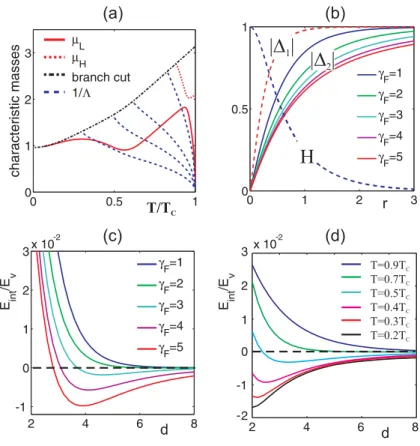
The examples from ref.22 of the temperature dependencies of the masses µ
L,H(T) are shown
in the Fig.2. The evolution of the masses µL,H is shown in the sequence of plots Fig.2(a)-(d) for
λJ increasing from the small valuesλJ ≪λ11, λ22 to the values comparable to intraband coupling
λJ ∼ λ11, λ22. The regime with two massive modes is exactly the same as the given by a
two-component GL theory. In this model, at very low temperatures there exists only one massive mode
µL(T) lying below the branch cut. As the interband coupling is increased above some critical value
the mass µH(T) disappears at all temperatures. In such a regime the asymptotic is determined
by a single coherence length and a branch cut with a continuous spectrum of scales. The branch
cut contribution is essentially a non-local effect which is not captured by GL theory. Therefore
one can expect growing discrepancies between effective GL solution and the result of microscopic
theory at low temperatures.
Besides justifying the predictions of phenomenological two-component GL theory18 the
micro-scopic formalism developed in Ref.(22) allows to describe type-1.5 superconductivity beyond the
validity of GL models. As shown on Fig.3a the function µL(T) is non-monotonic at low
tem-peratures. Therefore for a certain range of parameters in contrast with the physics of singe-band
superconductors the product of London penetration depth Λ andµLhas a strong and nonmonotonic
FIG. 2. Calculated in22 the inverse of coherence lengths (or masses)µ
L and µH (red solid lines) of the
composite gap function fields for the different values of interband Josephson couplingλJ andvF k= 1. By
black dash-dotted lines the branch cuts are shown. The coupling constants areλ11= 0.25,λ22= 0.213 and
λJ= 0.0005; 0.0025; 0.025 for plots (a-d) correspondingly. In (a) the blue dash-dotted lines correspond to
λJ = 0 showing two masses going to zero at two different temperatures. This corresponds to U(1)×U(1)
theory with two independently diverging coherence lengths. ForλJ6= 0 onlyµLgoes to zero atTc: this is in
turn a consequence of the fact that Josephson coupling breaks the symmetry down to singleU(1). However
when symmetry breaking is weak there is a local maximum of coherence length (local minimum of µL) at
lower temperature.
To demonstrate the type-1.5 superconductivity i.e. large-scale attraction and small-scale
repul-sion of vortices which originates from disparity of two coherence lengths, the inter-vortex interaction
energy Eint was calculated in.22 In Fig.3(c,d) Eint (normalized to the single vortex energy Ev) is
shown as a function of the distance between two vorticesd. The plots on Fig.3(c) clearly
demon-strate the emergence of type-1.5 behavior when the parameterγF =vF1/vF2, which characterizes
the disparity in band characteristics is increased.
The type-1.5 regime manifested in the appearance a non-monotonic behavior of Eint(d) when
one of the coherence length becomes larger than the magnetic field penetration length. The Fig.3(d)
showsEint for aU(1) two band superconductor that is type-2 nearTc and becomes type-1.5 near
superconductivity. The long-range attractive forces in type-1.5 regime are similar to the long-range
forces in type-1 superconductors, while short-range forces are similar to those in type-2
supercon-ductors. The physical origin and form of these interactions are obviously principally different from
the discussed in section IV microscopic-physics and non-locality-dominated intervortex forces in
superconductors near Bogomolnyi point.
B. Microscopic Ginzburg-Landau theory forU(1) two-band system.
Here we briefly outline the derivation of TCGL functional (22) from the microscopic equations
following.18 First we find the solutions of Eilenberger Eqs.(23) in the form of the expansion by
the amplitudes of gap functions |∆1,2| and their gradients |(npD)∆1,2|. Then these solutions are
substituted to the self-consistency Eq.(24). Using this procedure we find the solutions of Eqs.(23)
in the form:
fj =
∆j
ωn −
|∆j|2∆j
2ω3
n −
vF j
2ω2
n
(npD)∆j +
v2
F j
4ω3
n
(npD)(npD)∆j. (26)
andfj+(np) =fj∗(−np). Note that this GL expansion is based on neglecting the higher-order terms
in powers of|∆|and|(npD)∆|. Indeed this approximation naturally fails in a number of cases. The
regimes when it can be justified were determined in the work18 by a direct comparison to the full
microscopic model. Let us determine microscopic coefficients in the GL expansion. Substituting
to the self-consistency Eqs.(24) and integrating by θp we obtain
∆1 = (λ11∆1+λ12∆2)G+ (λ11GL1+λ12GL2) (27)
∆2 = (λ21∆1+λ22∆2)G+ (λ21GL1+λ22GL2) (28)
where
G= 2
Nd
X
n=0 πT
ωn
; X=X
n=0 πT ω3
n
(29)
GLj =X
vF j2 4 D
2∆
j− |∆j|2∆j
!
(30)
Expressing GLi from the equations above we obtain
n1GL1 =n1
λ22 DetˆΛ −G
∆1−
λJn1n2
DetˆΛ ∆2 (31)
n2GL2 =n2
λ11 DetˆΛ −G
∆2−λJn1n2
d
T/T
C
H
|D |
2|D |
1r
d T=0.9TC T=0.7T T=0.5T T=0.4T T=0.3T T=0.2T C C C C C ( )d
( )b
( )c ( )a
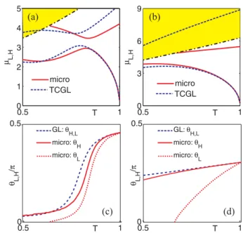
FIG. 3. Calculated in ref.22 (a) the inverse of coherence lengths (or masses)µ
L and µH (red solid and
dotted lines) of the composite gap function fields and inverse London penetration (blue dashed lines) for
the different values of ΛµL(Tc)/ √
2 = 1; 2; 3; 5. Scales above the black dash-dotted line are contained in
a branch-cut contribution. (b) Distributions of magnetic fieldH(r)/H(r= 0), gap functions |∆1|(r)/∆10
(dashed lines) and |∆2|(r)/∆20 (solid lines) for the coupling parameters λ11 = 0.25, λ22 = 0.213 and
λ21 = 0.0025 and different values of the band parameter γF = 1; 2; 3; 4; 5. (c,d) The interaction energy
Eint between two vortices normalized to the single vortex energyEv as function of the intervortex distance
d. In panel (c) the pairing constants are the same as in (d) andT = 0.6Tc. In panel (d)λii are the same as
in (c) but λ21 = 0.00125, and γF = 1. The panel (d) shows that when, at lower temperature, one of the
coherence lengths becomes larger than the magnetic field penetration length, the system falls into type-1.5
regime. The strength on the attraction grows as temperature becomes lower. The inter vortex distance
corresponding to minimum of interaction potential is strongly temperature dependent even below 0.5Tc. It
diminishes when temperature is decreased which should result in vortex cluster shrinkage with decreasing
The system of two coupled GL Eqs.(31) can be obtained minimizing the free energy provided the
coefficients in Eq.(22) are given by
ai =ρni(˜λii+ lnT −Gc) (33)
γ =ρn1n2λJ/DetˆΛ
bi=ρniX/T2
Ki=vF i2 bi/4
whereλJ =λ21/n1 =λ12/n2. Note that the expression forKi in Ref.18an extra coefficientρ. The
temperature is normalized to the Tc. Here X= 7ζ(3)/(8π2) ≈0.11, ¯λij =λ−ij1 and Gc =G(Tc) is
determined by the minimal positive eigenvalue of the inverse coupling matrix ˆλ−1 :
Gc =
Trλ−√Trλ2−4Detλ 2Detλ .
We have used the expression G(T) =G(Tc)−lnT. Near the critical temperature lnT ≈ −τ and
we obtain
ai=αi(T−Ti) (34)
αi=niλJ (35)
Ti= (1 +Gc−λ˜ii). (36)
In the above procedure of GL expansion leading to the system (31) we assumed both the
eigenvalues of the coupling matrix ˆλare positive.
C. Temperature dependence of coherence lengths.
Coherence lengths are given by the inverse masses of linear modes. First we investigate the
asymptotic behaviour of the superconducting gaps formulated in terms of the linear modes of the
density fields both in TCGL and microscopic theories described in the previous section. To find
the linear modes we follow the procedure described in the section (III) using the GL model with
expansion coefficients (33). Let us setK1=K2 which can be accomplished by rescaling the fields
∆1,2. Then the corresponding Hessian matrix (5) can be diagonalized with the k-independent
rotation introducing the normal modes χβ = Uβi(∆i−∆i0) where β = L, H and i = 1,2. The
rotation matrix ˆU is characterized by the mixing angle7,22 as follows:
ˆ U =
cosθL sinθL
−sinθH cosθH
Note that in accordance with the results of section (III) the TCGL theory yields identical values
of two mixing angles θL =θH = Θ where Θ is given by the Eq.(20). However, in general, outside
the region where GL expansion is accurate, the exact microscopic calculation of asymptotic yields
deviations θH 6=θL. This is discussed in Ref.18
The fieldsχL,H corresponding to the linear combinations of ∆1,2 vary at distinct lengths: ξH =
1/µH andξL= 1/µL. They constitute coherence lengths of the TCGL theory (22) and characterize
the asymptotic relaxation of the linear combinations of the fields ∆1,2, the linear combinations are
represented by the composite fields χL,H.
With the help of Eqs.(33) for GL coefficients obtained from microscopic theory we can study the
temperature dependencies of the coherence lengths characterizing the asymptotic relaxation of the
gap fields and compare them to the temperature dependence of coherence lengths in full microscopic
theory. Since the system in question breaks only one symmetry, then at critical temperature only
one coherence length can diverge while the second coherence should stay finite. Infinitesimally
close to critical temperatureT =Tc−0 the divergent coherence length has the following standard
mean-field behaviorξL = 1/µL ∼1/τ1/2, where τ = 1−T /Tc. The contribution of another linear
mode in the theory sets the scale which is proportional toξH = 1/µH. It remains finite atT =Tc.
But the amplitude of this mode rapidly vanishes in that region T = Tc −0. In Fig.(4)a,b the
temperature dependence of masses µL,H is plotted comparing the results of the full microscopic22
and microscopically derived TCGL theories.18It is shown for the cases of weak and strong interband
coupling in Fig.(4)c,d. We have found that TCGL theory describes the lowest characteristic mass
µL(T) (i.e. the longer coherence length) with a very good accuracy nearTc [compare the blue and
red curves in Fig. (4)a,b]. Remarkably, when interband coupling is relatively weak [Fig.(4)c] the
“light” mode is quite well described by TCGL also at low temperatures down toT = 0.5Tc around
which the weak band crosses over from active to passive (proximity-induced) superconductivity.
Indeed the τ parameter is large in that case. Nonetheless if the interband coupling is small one
does have a small parameter to implement a GL expansion for one of the components. Namely
one can still expand, e.g. in the powers of the weak gap |∆2|/πT ≪ 1. On the other hand for
the “heavy” mode we naturally obtain some discrepancies even relatively close to Tc, although
TCGL theory gives qualitatively correct picture for this mode when the interband coupling is not
too strong. More substantial discrepancies between TCGL and microscopic theories appear only
at lower temperatures or at stronger interband coupling [Fig.(4)d] where the microscopic response
function has only one pole, while TCGL theory generically has two poles. Note that these expected
the type-1.5 regime long-range attractive forces are governed by core-core interaction which range
is set by the larger coherence length (lighter mode).
The microscopic two-band GL expansion discussed in this section has straightforward
general-ization to N-component expansions in N-bandU(1) models.49 For a discussion of microscopic GL
expansion in more complicated states such as s+is that break multiple symmetries see.9,49
( )a ( )b
( )c ( )d
FIG. 4. (a) and (b) Comparison of field masses (inverse coherence lengths) given by full microscopic (solid
lines), and microscopically-derived TCGL (dotted) theories. The microscopic parameters are λ11 = 0.5,
λ22 = 0.426 and λ12 = λ21 = 0.01; 0.1 for (a,b) correspondingly. The yellow shaded region above the
dashed-dotted line shows the continuum of length scales determined by a branch-cut contributions which
are specific to the microscopic theory and are not captured by the TCGL description. (c,d) Comparison of
the mixing angle behaviour given by the exact microscopic (red lines) and microscopically derived TCGL
theories (blue line). Note that the larger coherence length has a maximum as a function of temperature
deep below Tc near the crossover to the regime when the weak band superconductivity is induced by an
interband proximity effect (the corresponding inverse quantity µL has a minimum). This non-monotonic
coherence length behavior is more pronounced at weak interband coupling and disappears at strong interband
coupling.22 A multiband system with weak interband interaction can easily fall into type-1.5 regime near
that crossover temperature. Panels (b) and (d) show a pattern how the TCGL theory starts to deviate from
the microscopic theory at lower temperature when interband coupling is increased. Parameters are the same
VI. SYSTEMS WITH GENERIC BREAKDOWN OF TYPE-1/TYPE-2 DICHOTOMY
In this section we discuss the simplest situations of generic type-1/type-2 dichotomy breakdown.
One example is superconducting systems that exhibit a phase transition from U(1) to U(1)×
U(1) state (or similar transitions between the states with broken higher symmetries), such as
the theoretically discussed superconducting states of liquid metallic hydrogen or deuterium,11 or
models involving mixture of protonic and Σ− hyperonic condensates in neutron stars,13 as well
as microscopic certain interface superconductors.33 Indeed at such a transition the magnetic field
penetration length remains finite but there is a divergent coherence length due to the breakdown
of additional symmetry (if the phase transition is continuous). Also the mode associated with
the divergent coherence length looses its amplitude at the phase transition. Therefore near this
transition one of the coherence lengths is the largest length scale of the problem and the system
can only be either a type-1 or type-1.5 superconductor.
Similar but more subtle situation takes place at the transition fromstos+isstate.10Thes+is
superconductor breaks additional Z2 symmetry and there is a corresponding diverging coherence
length in the problem. An important generic aspect of thes+issuperconducting states is that the
density excitations are coupled with the phase difference excitations in the linear theory.10 One of
the mixed phase-difference–density mode gives raise to a divergent coherence length at that phase
transition. Thus such a system can be either type-1 or type-1.5 near the transition fromstos+is
state. We discuss this example in more detail in Section VIII.
VII. STRUCTURE OF THE VORTEX CLUSTERS IN TYPE-1.5 TWO-COMPONENT SUPERCONDUCTOR.
In this section, following Ref.23 we consider in more detail the full non-linear problem in
two-component Ginzburg-Landau models, with and without Josephson coupling η which directly
cou-ples the two condensates (for treatment of other kinds of interband couplings see,7 for microscopic
derivation of the coefficients see Sec.IV). Whenη= 0 the condensates are coupled
electromagneti-cally. When there is non-zero interband Josephson coupling, the phase difference is associated with
a massive mode with massp η(u2
1+u22)/u1u2.
F = 1 2
X
i=1,2 "
|(∇+ieA)ψi|2+ (2αi+βi|ψi|2)|ψi|2
# +1
2(∇ ×A) 2
−η|ψ1||ψ2|cos(θ2−θ1) (38)
Since the Ginzburg-Landau model is linear, in general intervortex interaction is
consid-ered above, does not in general apply. Below we discuss the importance of complicated non-pairwise
forces between superconducting vortices arising in certain cases in multicomponent systems.23,43,44
These non-pairwise forces in certain cases have important consequences for vortex clusters
forma-tion in the type-1.5 regime.
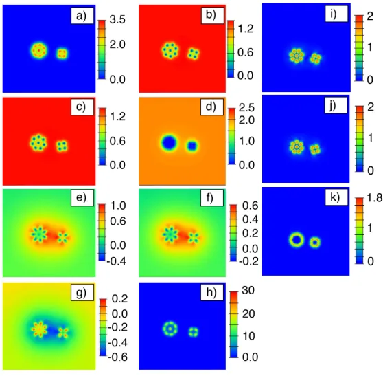
FIG. 5. Ground state of Nv = 9 flux quanta in a U(1)×U(1) type-1.5 superconductor (i.e. η = 0).
The parameters of the potential being here (α1, β1) = (−1.00,1.00) and (α2, β2) = (−0.60,1.00), while
the electric charge is e = 1.48 (in these units the electric charge value parameterises London penetration
length). The displayed physical quantities areathe magnetic flux density,b(resp.c) is the density of the first (resp. second) condensate|ψ1,2|2. d(resp.e) shows the norm of the supercurrent in the first (resp. second)
component. Panel f is Im(ψ∗
1ψ2) ≡ |ψ1||ψ2|sin(θ2−θ1) being nonzero when there appears a difference
between the phase of two condensates. The solution shows that clearly there is vortex interaction-induced
phase-difference gradient which contributes to non-pairwise intervortex forces. Parameters are chosen so that
the second component has a type-1 like behavior while the first one tends to from well separated vortices.
The density of the second band is depleted in the vortex cluster and its current is mostly concentrated on
the boundary of the cluster (see Ref.23).
Fig. 5 and Fig. 6 show numerical solutions for N-vortex bound states in several regimes (for
technical details see Appendix of23). The common aspect of the regimes shown on these figures
is that the density of one of the components is depleted in the vortex cluster and has its current
mostly concentrated on the boundary of the vortex cluster (i.e. has a “type-1”-like behavior). At
the same time the second component forms a distinct vortex lattice inside the vortex cluster (i.e.
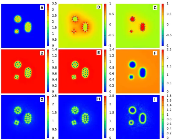
FIG. 6. Elongated ground state cluster of 18 vortices in a superconductor with two active bands. Parameters
of the interacting potential are (α1, β1) = (−1.00,1.00), (α2, β2) = (−0.0625,0.25) while the interband
coupling is η = 0.5. The electric charge, parameterizing the penetration depth of the magnetic field, is
e = 1.30 so that the well in the nonmonotonic interacting potential is very small. In this case there is
visible admixture of the current of second component in vortices inside the cluster, though its current is
predominantly concentrated on the boundary of the cluster.
Next we report the regime where the passive second band (i.e. with positive α2) is coupled to
the first band by strong Josephson coupling η = 7.0 (shown on Fig. 7). This coupling imposes
a strong energy penalty both for disparities of the condensates variations and for the difference
between phases of the condensates. In this regime there are also relatively strong non-pairwise
intervortex forces favouring chain-like vortex arrangements compared to compact clusters.23We get
a relatively flat and complicated energy landscape for multi-vortex configurations and the outcome
of the energy minimization strongly depends on initial configuration. Simulations whose outcome
is compact clusters like Fig.5and Fig.6are clearly ground states, since various initial guesses lead
to similar final configurations. Simulating systems like in Fig.7 is less straightforward. Numerical
evolution in these systems is extremely slow because of the complicated energy landscape. The
final state strongly depends on the initial field configuration, indicating the configuration is not
the ground state, but a “quasi-stationary” bound state with a very slow evolution. Formation of
highly disordered states and vortex chains due to the short-range nature of the attractive potentials
spite of the use of a fine numerical grid. Another example of systems that are generally more
inclined to posses non-pairwise intervortex forces that promote vortex-stripes are superconducting
condensates with phase separation.43
The Fig. 7 shows the typical non-universal outcome of the energy minimization in this case. A
striking feature here is formation of vortex stripe-like configuration, in contrast with the ground
state expected from the two-body forces in this system. Namely the axially symmetric two-body
potentials with long range attraction and short-range repulsion (which we have in this case) do
not allow ground states with stripe formation. In that regime the formation of vortex stripes and
small lines is aided by the repulsive non-pairwise intervortex interactions.23
Note that even in this regime, the non-linear effects in caused by intervortex interaction result
in self-induced gradients of the phase difference, in spite of the strong Josephson coupling.
When stray fields are taken into account in thin films, they give repulsive inter vortex interaction
at very long distances, while vortices can retain attractive interaction at intermediated length
scales. That gives raise to various hierarchical structures such as lattices of vortex clusters or
vortex stripes.39,64The study of dynamics demonstrated that such vortex systems can form vortex
glass phase.65This is in contrast to type-2 superconductors where vortex glass can appear only in
the presence of vortex pinning and not in clean samples.
VIII. MACROSCOPIC SEPARATION IN DOMAINS OF DIFFERENT BROKEN SYMMETRIES IN TYPE-1.5 SUPERCONDUCTING STATE.
As discussed above a system with non-monotonic intervortex interaction potentials allow a state
with macroscopic phase separation in vortex droplets and Meissner domains. In type-1.5
super-conductors this state can also represent a phase separation into domains of states with different
broken symmetries. In this section we will give two different examples of how such behavior arises.
Note that in multicomponent superconductors some symmetries are global (i.e. associated with
the degrees of freedom decoupled from vector potential) and some are local i.e. associated with the
degrees of freedom coupled to vector potential. As is well known, in the later case the concept of
spontaneous symmetry breakdown is not defined the same way as in a system with global symmetry.
However below, for brevity we will not be making terminological distinctions between local and
FIG. 7. A bound state of an Nv = 25 vortex configuration in case when superconductivity in the second
band is due to interband proximity effect and the Josephson coupling is relatively strong η = 7.0. The
initial configuration in this simulation was a giant vortex. Other parameters are (α1, β1) = (−1.00,1.00),
(α2, β2) = (3.00,0.50),e = 1.30. For the simulations, like the one shown on Fig. 6 the stopping criterion
of energy minimization was when relative variation of the norm of the gradient of the GL functional with
respect to all degrees of freedom to be less than 10−6. Here the situation is slightly different from that
shown on two previous figures. Clearly in the shown above configuration the ground state was not reached.
However the interaction potentials a such that the evolution at the later stages becomes extremely slow.
The number of energy minimization steps in this case was order of magnitude larger than what was required
for convergence in the previous regimes. This signals that in similar systems vortex stripes will be likely to
form (relative to more compact vortex clusters) for kinetic reasons as well as due to thermal fluctuations
A. Macroscopic phase separation into U(1)×U(1) and U(1) domains in type-1.5 regime.
Consider a superconductor with brokenU(1)×U(1) symmetry, i.e. a collection of independently
conserved condensates with no intercomponent Josephson coupling. As discussed above, in the
vortex cluster state, in the interior of a vortex droplet, the superconducting component which has
vortices with larger cores is more depleted. InU(1)×U(1) system the vortices with phase windings
in different condensates are bound electromagnetically, resulting in an asymptotically logarithmic
interaction potential with a prefactor proportional to|ψ1|2|ψ2|2/(|ψ1|2+|ψ2|2),50and even weaker
interaction strength at shorter separations.
is not completely depleted, its density is suppressed and as a consequence the binding energy
between vortices with different phase windings (∆θ1 = 2π,∆θ2 = 0) and (∆θ1 = 0,∆θ2 = 2π) can
be arbitrarily small. Moreover the vortex ordering energy in the component with more depleted
density is small as well. As a result, even tiny thermal fluctuation can drive vortex sublattice
melting transition11,66 in a large vortex cluster. In that case the fractional vortices in weaker
the component tear themselves off the fractional vortices in strong the component and form a
disordered state. Note that the vortex sublattice melting is associated with the phase transition
fromU(1)×U(1) toU(1) broken symmetries.11,66Thus, a macroscopically large vortex cluster can
realise a domain of U(1) phase (associated with the superconducting state of strong component)
immersed in domain of vortexless U(1)×U(1) Meissner state. If the magnetic field is increased,
the system will go from the vortex clusters state (with coexistingU(1)×U(1) andU(1) domains)
to a U(1) vortex state.
B. Macroscopic phase separation in U(1) and U(1)×Z2 domains in three band type-1.5 superconductors.
In this subsection we discuss an example of vortex clusters in three-band superconductors that
locally break additional Z2 symmetry forming “phase-frustrated” states. Such superconductors
also allow the coexistence of domains with different broken symmetries in the ground state. The
minimal GL free energy functional to model a three-band superconductor is
F = 1
2(∇ ×A)
2+ X
i=1,2,3 1 2|Dψi|
2+α
i|ψi|2+
1 2βi|ψi|
4+ X
i=1,2,3 X
j>i
ηij|ψi||ψj|cos(ϕij). (39)
Here the phase difference between two components are denoted ϕij =θj−θi. Microscopic
deriva-tions of such models describings+is superconducting states can be found in.9,49
Systems with more than two Josephson-coupled bands can exhibit phase frustration.8–10,67,68
Forηij <0, a given Josephson interaction energy term is minimal for zero phase difference (we then
refer to the coupling as “phase-locking” ), while when ηij >0 it is minimal for a phase difference
equal to π (we then refer to the coupling as “phase-antilocking” ). Two-component systems with
bilinear Josephson coupling are symmetric with respect to the sign changeηij → −ηij as the phase
difference changes by a factor π, for the system to recover the same interaction. However, in
systems with more than two bands there is generally no such symmetry. For example if a
three-band system hasη >0 for all Josephson interactions, then these terms can not be simultaneously