This is a repository copy of A dynamic microsimulation framework for generating synthetic
spatiotemporal crime patterns.
White Rose Research Online URL for this paper:
http://eprints.whiterose.ac.uk/128602/
Version: Accepted Version
Proceedings Paper:
Adepeju, MO orcid.org/0000-0002-9006-4934 and Evans, A (Accepted: 2018) A dynamic
microsimulation framework for generating synthetic spatiotemporal crime patterns. In:
GISRUK 2018 Proceedings. 26th GIScience Research UK Conference (GISRUK 2018),
17-20 Apr 2018, Leicester. . (In Press)
[email protected] https://eprints.whiterose.ac.uk/
Reuse
Items deposited in White Rose Research Online are protected by copyright, with all rights reserved unless indicated otherwise. They may be downloaded and/or printed for private study, or other acts as permitted by national copyright laws. The publisher or other rights holders may allow further reproduction and re-use of the full text version. This is indicated by the licence information on the White Rose Research Online record for the item.
Takedown
If you consider content in White Rose Research Online to be in breach of UK law, please notify us by
A dynamic microsimulation framework for generating synthetic
spatiotemporal crime patterns
Monsuru Adepeju
*1and Andrew Evans
†11School of Geography, University of Leeds, LS2 9JT, United Kingdom
January 12, 2018
Summary
The significance of synthetic crime datasets in criminological research cannot be underestimated, as real crime datasets are usually unavailable in many policing jurisdictions, due to reasons such as
privacy concerns and the lack of shareable data formats. This study introduces a dynamic microsimulation framework by which a specified spatiotemporal crime pattern can be synthesised. A
case study presented compares a real crime dataset with the synthesised datasets, and found certain spatiotemporal similarities between them. The developed model has the potential for wider
applications in criminology, given some identified areas of improvement.
KEYWORDS: crime patterns, dynamic microsimulation, synthetic crime, spatiotemporal pattern
1. Introduction
Crime is an inherently human phenomenon; a complex interaction between the criminals, victims, police and the surrounding environmental factors (Cohen and Felson, 1979; Brantingham and Brantingham, 1993). Due to the complex nature of human behaviour in relation to its environment, it is often difficult to synthesise these interactions in a computer environment, in order to generate synthetic crime datasets, which are often required for many criminological studies. Given the fact that real crime datasets are usually unavailable in many policing jurisdictions, due to reasons such as privacy concerns and the lack of shareable data formats, synthetic datasets may provide alternative datasets for a lot of criminological research. In previous studies, synthetic datasets have been used to examine criminological theories (Chastain et al., 2016) as well as for investigating the performance of analytical methods (Shiode and Shiode, 2013). For example, the detection capability of a cluster detection algorithm was assessed using artificially-induced crime hotspots (Shiode and Shiode, 2013). Our goal, in this study, is similar; to develop a simulation framework by which a synthetic crime dataset can be generated, with a defined spatiotemporal pattern. The novelty of our study lies in the integration of complex human behaviours with crime the underlying environmental factors to model the spatiotemporal point patterns, within a heterogeneous network landscape. The detection or identification of such as a pattern may subsequently be used to assess the performance of crime hotspot algorithms.
In this study, we adapted a dynamic microsimulation model (DMM) that was originally used in the field of ecology for simulating the interactions between foraging animals and their environments (Morales et al., 2004; McClintock et al., 2012). In this model, the behavioural movement of an object can be simulated in relation to progressions in time, allowing a specified spatiotemporal pattern to be synthesised (Li and O’Donoghue, 2013). The DMM is built on certain assumed movement parameters and a transition matrix - a time-nonhomogeneous Markov chain with a limited number of behavioural states, incorporated to control the potential behavioural changes of an offender in relation to some theoretical considerations. An offender is then allowed to transit systematically across three assumed behavioural states, namely; the ‘exploratory state’, the ‘motivated state’ and the ‘offending state’. The
model parameters were carefully chosen to enable some localised spatiotemporal patterns to be synthesised.
The resultant spatial and temporal crime patterns are compared with real crime datasets using repeat pattern profiles (Johnson et al., 1997) and Ripley K-test (Ripley, 1988), respectively. These statistics are generally used to assess the theory of repeat victimisation of crime; the central idea of any spatiotemporal crime pattern analysis. The repeat victimisation theory states that if a target such as building is victimised, the targets within a relatively short distance of the original target have an increased risk of being victimised over a limited period of time —varying from days to weeks of the original victimisation taking place (Farrel and Pease, 1993; Bowers and Johnson, 2005). This study represents a preliminary effort towards the development of a general-purpose simulation framework by which synthetic datasets of varying spatiotemporal characteristics can be generated.
2. A Dynamic Microsimulation framework of crime
The proposed DMM framework comprises a latent variable model, where an object switches between discrete (unobserved) movement behaviour states , where each state is a collection of movements between consecutive positions ( ) and ( ) for each time step . The framework follows the Morales et al. (2004) model by selecting a Weibull distribution for the step length ( ) and a wrapped ( ) Cauchy distribution for the direction ( ) of movement. The movement process model is therefore, a discrete-time, continuous space, multi-state movement model with step length Weibull and direction Cauchy .
Then, we have the following probability density function:
exp (5)
and
cos
(6)
For , , , , , and Assuming
independence between step length and direction within each movement’s behavioural state, the joint likelihood for and , conditioned on the latent state variable , is:
(7)
In order to switch between different states, a categorical distribution is assigned to the latent state variable . In its simplest form, every time step may be assigned to a movement behaviour state, independent of the previous state:
Categorical (8)
Such that Pr , where is the fixed probability of being in state at time , and
For this study, we define three movement behavioural states, namely; (1) “exploratory” - describing a sequence of undirected and random movements, (2) “motivated” – also undirected but
Categorical (9)
And Pr , for , where is the probability of switching from state at time to state at time .
2.1. Parameterisation of the model for South Chicago area
Two parameters, namely; the spatial range, K, and the Markov transition probabilities, are used to condition the DMM, in order to generate localised spatial patterns and cyclic temporal fluctuations, respectively. The spatial range is a radius, measured from an offender’s origin, within which an offender is expected to operate. A list of K (200m, 400m, … , 1000m) was created. The direction , is continuously re-adjusted if , where is the distance between the origin of an offender and its next potential location. This allows the offender to be kept within its spatial range. The transition matrix is defined as Pr(0.05, 0.0001, 0.05, 0.0282, 0.05, 0.05), allowing a transition to be made to the
‘offending state’ at an approximate step length counts equivalent to 14 days. The difference between
the ‘exploratory state’ and the ‘motivated state’ lies in the directional values ( ) of 0.3 specified for the latter, enabling a slightly ‘directed’ movement to be made while the offender is in this state. The directional values ( ) of 0.8 is specified for the ‘offending state’, enabling an offender to move in an almost opposite direction as soon as an offence is committed.
We used the SimRiv package in R (Quaglietta and Porto, 2017), which allows a movement constraint to be integrated in the form of a heterogeneous network landscape. A resistance raster map built comprises a buffered street network and a background, with resistance values of 0 and 0.95, respectively. This allows the movements to be restricted only to the street network.
Figure 1. (a) Land use map and (b) Resistance map built, for South Chicago area
The offenders’ origins are specified using the locations of the residential buildings, randomly selected amongst the three categories of residential land use (Figure 1 (a)), based on the visual inspection of the real datasets (see section 3). A total of 300 offenders were synthesised during each simulation, with varying spatial range, K. The parameter combination ensures that similar total number of crimes are generated for each value of K.
3. Comparative analysis of the real and synthetic datasets
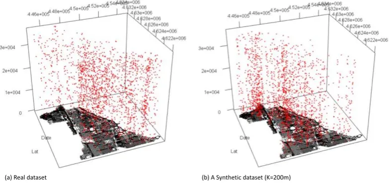
[image:4.595.109.490.396.584.2]3.1. 3D point distribution
Figure 2a shows the 3D point distribution of the real dataset, while figure 2b shows the 3D point distribution of a synthetic data, when K=200m.
Figure 2. 3D point distribution. (a) real dataset and (b) a synthetic dataset (where K=200m)
The most noticeable difference between the two point distributions is the relatively higher point densities in the south-east corner and the north-west corner of the study area, for the real dataset and the synthetic dataset, respectively. The difference can be attributed to the disproportionate higher distribution of the offenders at the north-west corner of the area during the simulation. This can be improved with a more accurate specification of origins for the offenders.
3.2 The spatial and temporal patterns
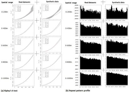
Figure 3a and Figure 3b show the results of the Ripley’s K-test using R-Spatstat package (Baddeley et al., 2015) and the repeat pattern profiles (Johnson et al. 1997), respectively. For convenience, the baseline distributions for the K-tests was defined as an inhomogeneous Poisson process, through the fitting of a Gaussian density model. For the real datasets, different spatial bandwidths (i.e. 200m, 400m, .., 1000m) are used to generate different test plots, while for the synthetic dataset, the value of K that was used for simulating each dataset is employed for fitting the Gaussian density model.
Real datasets
[image:5.595.100.492.133.317.2]
Figure 3. (a) Ripley K-test for spatial clustering analysis, and (b) the repeat pattern profiles for
temporal clustering analysis, for both the real and the synthetic dataset. Inhomogeneous Poisson model as the baseline distribution. Different arbitrary values of K is used for defining the bandwidth
for the baseline distribution of the real datasets, while the value of K used in the simulation of the synthetic dataset is used for defining the bandwidth for the baseline distribution of the synthetic
datasets. The black (solid) lines represent the observed estimates, while the red (dotted) lines represent the mean simulated estimates, bounded by the maximum and the minimum simulated estimates, across all distances. The repeat pattern profiles of both the real dataset and the synthetic
datasets are estimated at 1-day temporal lag distances up to 60 days. Edge corrections are implemented in both cases.
In all the cases, both the observed and the inhomogeneous Poisson model appear closer to one another. For the real dataset, both models appear to describe each other better, at spatial bandwidths of 200m, 400m and 600m, while diverging at bandwidths of 800m and 1000m. For the simulated datasets, the theoretical estimates only appear to describe the observed estimates as K and r approach each other. For example, at K=400m, both estimates appear to coincide at around r=400m and 600m. However, both patterns start to diverge very significantly at larger values of K. This explains the fact that as the spatial range increases, the spatial coverages of the offenders begin to overlap one another, thereby producing interwoven point distribution.
[image:6.595.72.525.85.408.2]points start to interact, giving rise to spatiotemporal interactions. We can say that the real dataset is less
‘well-defined’, primarily because the assumption of the uniform spatial range (K) does not hold. Lastly, the pattern profiles of the synthetic datasets at 0-800m and 0-1000m look similar to the real dataset. This is primarily due to the spatiotemporal interactions in the activities of the offenders, as they are able to cover more distance, and tends to produce similar patterns as the real datasets.
4. Further work
This study represents a preliminary stage of our model building. The goal is to develop a general-purpose framework that will allow different theory-based spatiotemporal patterns to be synthesised. In order to achieve this goal, we intend to incorporate different environmental crime-related factors into the model. Furthermore, a simulated offender should be able to evaluate risk and benefits, and also learn from past activities.
5. Acknowledgements
This work was funded by the UK Home Office Police Innovation Fund, through the project “More with
Less: Authentic Implementation of Evidence-Based Predictive Patrol Plans”.
6. Biography
Dr. Monsuru Adepeju is a Research Fellow in Geocomputation at the University of Leeds. His research interests cover predictive policing, geostatistics and application of GIS to social-economic areas such as crime and health. His current research focuses on developing dynamic microsimulation frameworks for model testing in crime and transport domains.
Dr. Andrew Evans is a Senior Lecturer in GIS/Computational Geography. His primary interest is in developing 'Artifical Intelligence' solutions in geography (for example, in social modelling). He is also working to develop new technologies to aid democracy and people's understanding of space, such as 'fuzzy' mapping software
References
Baddeley A, Rubak E and Turner R (2015). Spatial Point Patterns: Methodology and Applications with R. London: Chapman and Hall/CRC Press.
Bowers K J and Johnson S D (2005). Domestic burglary repeats and space-time clusters the dimensions of risk. European Journal of Criminology, 2(1), 67-92.
Brantingham P L and Brantingham P J (1993). Nodes, paths and edges: Considerations on the complexity of crime and the physical environment. Journal of Environmental Psychology, 13(1), 3– 28.
Cohen L and Felson M (1979). Social change and crime rate trends: A routine activity approach. American Sociological Review, 44, 588–608.
Farrell G and PEASE K (1993). Once bitten, twice bitten: Repeat victimisation and its implications for crime prevention.
Johnson S D, Bowers K and Hirschfield A (1997). New insights into the spatial and temporal distribution of repeat victimization. The British Journal of Criminology, 37(2), 224-241.
Li J and O'Donoghue C (2013). A survey of dynamic microsimulation models: uses, model structure and methodology. International Journal of Microsimulation, 6(2), 3-55.
McClintock B T, King R, Thomas L, Matthiopoulos J, McConnell B J and Morales J M (2012). A general discrete time modeling framework for animal movement using multistate random walks. Ecological Monographs, 82(3), 335-349.
relocation data: building movement models as mixtures of random walks. Ecology, 85(9), 2436-2445.
Quaglietta L and Porto M (2017). SiMRiv: Individual-Based, Spatially-Explicit Simulation and Analysis of Multi-State Movements in River Networks and Heterogeneous Landscapes_. R package version 1.0.2
Ripley B (1988). Statistical Inference for Spatial Processes. Cambridge University Press.
Shiode S and Shiode N (2013). Network-based space-time search-window technique for hotspot detection of street-level crime incidents. International Journal of Geographical Information Science, 27(5), 866-882.