THE PRODUCTION OF PULSED NOZZLE FLOWS IN A SHOCK TUBE
by
Neil Robert Mudford
A thesis submitted for the degree of Doctor of Philosophy at the Australian National University
Canberra
in the Acknowledgements and where credit is indicated by reference, is entirely my own work
Firstly, I would like to thank my supervisor, Dr. R. J. Stalker, for the invaluable help and guidance which he has given me during the time that we have worked
together. I am also indebted to him for the design of the hardware for the modification to the shock tunnel and for the original concept for the modification. I would also like to thank Dr. Hans Hornung and Dr. John Sandeman for their generous assistance, given on innumerable occasions.
There are many other people to whom I am indebted: to Mr. Roland French, Mr. Vic Adams and Mr. Gavin Spackman for their help in performing the experiments, maintaining the equipment and running the tunnel and shock tube safely and efficiently; to Mr. Ken Smith for his photographic work and the helpful advice he has given in this field;
to Mr. Len Batt and Mr. David King for repair and mainten ance of the electronic equipment; to the workshop staff of the Physics Department for the production of several pieces of apparatus all of which have been of high quality.
My thanks go also to my fellow post-graduate students, notably Doug Kewley, Nizar Ebrahim, Graham Caldersmith, John Baird and Mike Daffey, for the many
stimulating and helpful discussions we have had.
I extend my thanks to Ms. Julie Faux, not only for typing this thesis, but for going, with me, through all the traumas of its compilation.
Finally, I wish to express my appreciation to the Australian Government for their provision of a Commonwealth
A theoretical and experimental study has been made of short duration nozzle flows in a high enthalpy non-reflected shock tunnel.
A reduction in initial nozzle density, necessary for minimisation of the loss of steady test flow time due to starting processes in the nozzle, was achieved by creating a steady supersonic
flow in the nozzle prior to the arrival of the primary shock. A model of the nozzle starting processes in a non-reflected shock tunnel was developed from a model, due to Smith (1966), for these processes in a reflected shock tunnel. On the basis of this model a method of characteristics calculation and an analytic calculation were made. These calculations yielded predictions for the paths,
in the x-t plane, of the principal disturbances due to the nozzle starting processes.
A contoured nozzle was designed to produce a uniform, parallel, steady test flow in the test section, with minimum test
flow time losses.
An experimental programme was undertaken to observe both the shock tube and test section flows in the shock tunnel. This programme yielded information about the primary shock speed in the shock tube, the duration of test flow in the shocx tube, the paths in the x-t plane of the unsteady flow features in the nozzle flow, the steadiness, integrated refractivity and duration of the steady test section flow and the species present as impurities
in the flows.
The test gases used in the experiments were air, as a representative dissociating gas, and argon, as a representative
TABLE OF CONTENTS
ACKNOWLEDGEMENTS.
ABSTRACT.
CHAPTER 1. INTRODUCTION. 1
CHAPTER 2. STARTING PROCESSES IN THE NOZZLE. 5
2.1. Introduction. 5
2.2. The model. 7
2.3. The flowfield calculation. 8
2.3.1. Nonsteady Method of Characteristics. 9
2.3.2. Results of M.O.C. 11
2.3.3. The analytic model. 11
2.4. Theory and experiment. 14
2.5. Contact surface matching. 15
2.6. Minimum nozzle lengths. 16
CHAPTER 3. DESIGN OF THE NOZZLE. 18
3.1. Introduction. 18
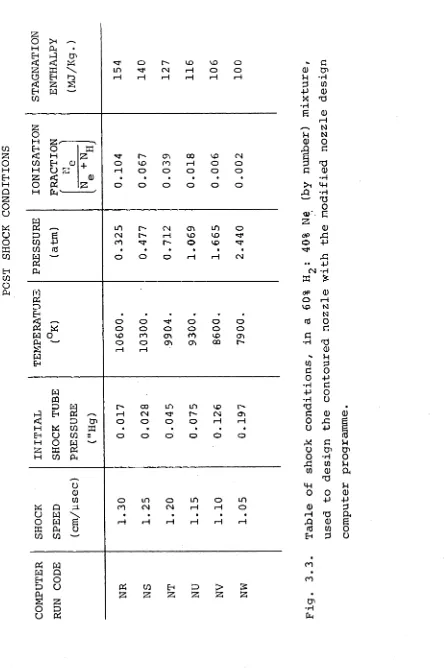
3.2. The nozzle design computer programmes. 19 3.2.1. The perfect gas programme. 19 3.2.2. The modified nozzle design programme. 22 3.3. The nozzle design proceedure. 28 3.4. Survey of minimum nozzle lengths. 31
3.5. Conclusion. 31
CHAPTER 4. THE EXPERIMENTAL CONFIGURATIONS. 32
4.1. The tunnel. 32
4.2. Gases. 33
4.3. shock tube flows 34
4.4. Test section flows. 35
4.4.1. The Image Converter Camera. 35 4.4.2. The exploding wire light source. 35 4.4.3. Emission spectra from the shock layer 36
on a cylinder. 37 4.4.5. Standoff distance of a flow on a
cylinder. 38
4.4.6. Interferometry. 38
4.4.7. Horizontal slit interferogrammes. 39 4.4.8. Vertical slit interferogrammes. 40 4.4.9. Framing photographs of body flows. 40 4.4.10. Stagnation pressures measurement. 41
CHAPTER 5. RESULTS AND DISCUSSION. 43
5.1. Shock speeds and initial pressures. 43
5.2. Duration of tube flow. 43
5.3. Pressure disturbances in the flow. 48 5.4. Existence of a prior, steady supersonic
flow. 51
5.5. Steady flow properties. 53
5.5.1. Introduction. 53
5.5.2. Treatment of the interferogrammes. 54 5.5.3. The horizontal slit interferogrammes. 56 5.5.4. The vertical slit interferogrammes. 58 5.5.5. The physical and chemical properties
of the steady air flows. 61
5.5.6. The physical and chemical properties
of the steady argon flows. 63
5.5.7. Body flows. 68
5.6. Emission and absorption spectra. 69
5.6.1. Emission spectra. 69
5.6.2. Absorption spectra. 70
CHAPTER 6. CONCLUSION. 71
LIST OF FIGURES.
. CHAPTER 1 . INTRODUCTION.
Studies in high velocity, hypersonic gas dynamics, have, for many years, been carried out with the aid of the reflect ed shock tunnel (e.g. Hertzberg et al (1961) Holder and
Schultz (1961)). The shock tube, from which the reflected shock tunnel is derived, is capable of producing hypersonic flows with higher stagnation enthalpies and higher densities than can be realised in the reflected shock tunnel. If
hypersonic flows with higher stagnation enthalpies and densit ies could be produced, several important phenomena, such as the effects of chemical reactions, radiation or electron thermal conductivity on a flowfield, could be studied more fully.
In the reflected shock tunnel, the primary shock in the shock tube is reflected at the end of the tube. The result ing high pressure reservoir of gas then passes into the hypersonic nozzle through a small hole in the end wall. The limitations of the reflected shock tunnel arise almost
entirely from the process of shock reflection.
By developing a non-reflected shock tunnel as a deriv ative of the shock tube, the limitations associated with shock reflection can be circumvented (Oertel (1969)). The primary shock in the non-reflected shock tunnel passes directly from the shock tube into the hypersonic nozzle.
Part of the flow which follows the shock is expanded through the nozzle in a steady expansion to produce a steady,
hypersonic flow in the test section.
The non-reflected mode of operation has three advantages over the reflected mode:
1. High densities. High test section densities are produced by high nozzle reservoir pressures. Because of the fact that the non-reflected tunnel avoids the entropy rise across a reflected shock, the nozzle reservoir pressure should be higher for the non-reflected tunnel than for the reflected tunnel. A comparison of this pressure for the reflected (P__) and non-reflected (P ) tunnels is shown in
R R KM
2
It was assumed in the calculations which produced the graph in Fig. 1.1 that the nozzle pressure in the reflected tunnel was the reflected shock pressure i.e. that the
tunnel was run at the tailored interface condition. However, for high enthalpy operation, the reflected tunnel must be run below the tajlored interface condition to avoid contamin ation of the test gas by the driver gas. This implies that the nozzle reservoir pressure is less than PD_. in the
reflected mode.
Stalker and Hornung (1969) have reported that the
plateau pressure, measured in the stagnation region of a high enthalpy reflected shock tunnel, was substantially below the calculated value.
In practice, therefore, the ratio of the nozzle pressure in the non-reflected mode to that in the reflected mode will be higher than that shown in Fig. 1.1.
A high test section density leads to a reduction in the relaxation length for chemical reactions. A number of
studies of flows in which non-equilibrium chemistry in a body flow causes significant changes in the flow density, over the dimensions of the body, have been carried out at the A.N.U, (Hornung and Sandeman (1974) , Kewley and Hornung
(1974)# Ebrahim and Hornung (1975)) . A reduction in the chemical relaxation length will allow the performance of a wider range of experiments of this type. As well as this, the higher densities in the non-reflected tunnel will aid the production of flows with high Reynolds Number.
2. High stagnation enthalpies. Studies by Logan (1972) have shown that substantial enthalpy losses occur, through radiation in the stagnation region, in the reflected tunnel at high stagnation enthalpies. For example, Logan showed that for a 5.7km/sec. primary shock into 2"Hg of argon, losses of up to 65% of the enthalpy occur in the stagnation region of a reflected tunnel. This loss is in addition to radiative energy losses from the gas behind the primary shock. Hornung and Sandeman (1974) confirmed Logan's results and
Between 40 and 45% of the stagnation enthalpy of the gas behind the primary shock in the tube is in the form of kinetic energy. This sets an upper limit for the radiative energy losses from flows in a non-reflected shock tunnel. The elimination of the shock reflection process in the shock tunnel therefore leads to a retention of a far greater
proportion of the stagnation enthalpy of the test gas.
The only losses through radiation are those occuring behind the primary shock.
3. Test gas purity. The interaction of a reflected shock wave and the boundary layer on the shock tube walls leads to mixing of the boundary layer gas with the test gas. Impurities from the shock tube walls are thereby introduced into the test flow. By contrast, the flow in the test sect ion of the non-reflected shock tunnel should be spectro scopically pure if the flow behind the primary shock in the tube is spectroscopically pure.
Another source of contamination of the test gas flow in a reflected shock tunnel is the flow of He driver gas along the shock tube walls after shock reflection. Davies and Wilson (1969)proposed this mechanism to explain the fact that He appeared in the test section flow a good deal earlier than would occur had the contact surface been leak-free.
Shock tube studies at the A.N.U. have shown that if the contact surface is stable there is only a small amount of mixing of the test and driver gases across the contact
surface in the tube. It is therefore reasonable to expect that there will be little He contamination in the test section flows in the non-reflected shock tunnel.
The only disadvantage of the non-reflected shock tunnel is the short duration of steady flow in the test section. An upper limit for the steady test section flow time is
4
end of the shock tube and evacuated the nozzle and test section. The shock tube flows in the facility at the A.N.U. are of higher stagnation enthalpy and shorter duration than those of Oertel. The short test times are not sufficient to allow successful removal of such a diaphragm.
Studies on a small, non-reflected shock tunnel (Stalker and Mudford (1973)) showed that the establishment of a steady, supersonic flow in the nozzle test section, prior to the arrival of the primary shock, increased the test flow time in the tunnel.This flow, which will be referred to through out this thesis as the Prior Steady Flow, is established by opening a valve between the test section, in which the
initial gas conditions are those of the shock tube, and an evacuated dump tank downstream of the test section. In this thesis the technique is applied to flows in a large shock tunnel (see Stalker and Hornung (1969) for details of the shock tube from which the tunnel is derived). It will be shown in the thesis that the reduction in density in the nozzle, due to the presence of the prior steady flow, is sufficient to ensure that the test time losses, due to the nonsteady starting processes, are minimized.
In Chapter 2, the nonsteady starting and finishing
processes in the nozzle flow will be discussed. An analytic model which may be used to calculate the trajectories of the features of interest in the nonsteady flow will be presented in this chapter.
The method used to design a nozzle which must be short, in order to ensure rapid starting of the nozzle flow, and yet produce a steady, uniform, hypersonic test section flow, is presented in Chapter 3.
In Chapter 4, the details of the experiments performed to observe the flows in the non-reflected shock tunnel are given.
The results of the experiments and discussion of the results are contained in Chapter 5.
CHAPTER 2 . STARTING PROCESSES IN THE NOZZLE. 2.1. INTRODUCTION.
A one dimensional shock wave propagating along a shock tube will travel at constant speed if the cross-sectional area of the tube, the density (and pressure and composition) of the gas ahead of shock and the pressure of the driver gas at the contact surface all remain constant. The gain
in momentum experienced by the initially quiescent test gas, as it passes through the shock wave, is balanced by the impulse of the driver gas at the contact surface. Under these circumstances, in the rest frame of the shock, there are no travelling pressure disturbances in the post shock gas.
However, if the shock wave passes into an expanding portion of the shock tube, such as a hypersonic nozzle, and the initial test gas density in the nozzle is the same as that in the upstream parts of the tube, then the shock will decelerate and a compressive pressure disturbance will
propagate upstream relative to the primary shock. The
reason for the deceleration of the primary shock is that an increase in the tube cross-sectional area leads to an
increase in the test gas mass to be accelerated per unit distance travelled by the shock. As well as this, the post primary shock pressure impulse is reduced by the area increase, because the post shock flow is supersonic for the shocks of interest.
ahead
If, on the other hand, the density^of the primary shock is reduced, while the cross-sectional area remains constant, the primary shock will accelerate and an upstream facing expansion wave will propagate into the post primary shock gas.
The shock acceleration is due to the decrease in the mass to be accelerated by the shock per unit distance travelled by the shock coupled with the constancy of the post primary
6
flow times available in the shock tube at high stagnation enthalpies.
C.E. Smith (1966) has made a study of the nonsteady processes which precede the establishment of a steady, or a near steady, flow in the nozzle of a shock tunnel operated in the reflected mode. By placing a diaphragm at the nozzle entrance, Smith was able to set the initial density in the nozzle to any desired value. He showed that, up to a point, the time for the nozzle flow to become steady, at a partic ular station, is reduced by a reduction in the initial press ure (density) in the nozzle.
It is not possible to place a diaphragm at the nozzle entrance of the non-reflected shock tunnel because the test flow is not of sufficient duration to successsfully rupture a diaphragm and remove the diaphragm material from the flow,
(see Chapter 5, section 5.2 for the test flow durations). However, it will be shown in this thesis, that the loss of
steady rest flow time, due to the nonsteady starting processes, can be minimised by the establishment of a steady, supersonic flow in the nozzle prior to the arrival of the primary shock. I shall refer to this pre-primary shock flow as the "prior steady flow".
The establishment of the prior steady flow is initiated by opening a valve between the downstream end of the test
section and the evacuated dump tank further downstream (see Chapter 4, section 4.1). Gas in the test section flows into the dump tank and an expansion wave travels upstream into the test section and the nozzle. After a time the flow becomes steady and is supersonic downstream of the nozzle entrance, where the flow is sonic.
The valve is opened by the recoil of the shock tube mech anism which occurs when the free piston moves forward off its launcher and begins to move down the compression tube. In Appendix A it is shown that there is sufficient time, between the valve opening and the arrival of the primary shock at the nozzle, for the prior flow to become steady. It is also
2.2. THE MODEL.
The model of the nonsteady starting flow field proposed by Smith, and supported by his experiments, needs only slight modification to be made applicable to the nozzle flow in the
non-reflected shock tunnel. There are three important diff erences between the operation of the reflected and non reflect ed shock tunnels, with regard to the nozzle flows. In the
reflected mode the final steady flow at the nozzle entrance is sonic; there is, initially, a diaphragm at the nozzle
entrance and the test gas flow does not encounter the reduced initial density field in the nozzle until downstream of the nozzle entrance. In the non rpf 1 pr'f pH mnrlp fho f i nal , ct-oarlw
head of this expansion wave travels upstream in the frame of reference of the primary shock, but travels downstream in the laboratory frame, because the post primary shock flow is supersonic in the laboratory frame. The primary shock contin ues to accelerate until it reaches a point, a short distance downstream of the nozzle entrance, where the influence of the growing nozzle cross-sectional area exceeds the influence of the decreasing density field. The primary shock then begins to decelerate and a compression wave is sent back into the post primary shock gas. The continuing deceleration of the primary shock, after this point, causes the compression wave to steepen, and, eventually, it forms into an upstream facing shock wave.
expan-sion wave. The head of the expansion wave is, in these cir cumstances, the upstream limit of the nonsteady flow field. After it has passed downstream of a particular station,
steady test flow conditions will exist at that station. If there is no prior flow in the nozzle, then the prim ary shock maintains its initial, constant speed until it
encounters the expanding section of the nozzle and begins to decelerate. Once again, a secondary shock wave forms in the manner described above. In this case, due to the absence of the upstream facing expansion wave, the secondary shock is the upstream limit of the nonsteady starting flow field.
2.3. THE FLOW FIELD CALCULATIONS.
Calculations have been made of the trajectories of the starting shocks and the other flow features present in the nonsteady starting flowfield. From the results of these calculations, the effect of the presence of a prior steady flow in the nozzle can be assessed, and estimates made of the loss, if any, of the steady test flow time due to the presence of the secondary shock.
Two calculation methods were used to solve the problem of the nonsteady flowfield. The first method was a method of characteristics calculation, using perfect gas equations and a constant ratio of specific heats throughout. This calculation yielded estimates for the separation distance between the primary and secondary shocks in the nozzle and
the variation of gas flow properties over the whole non steady flowfield. However, it could not, in its modelling of the flow, take account of the presence of real gas
effects, such as chemical dissociation, ionisation and energy losses due to radiation.
The second method calculated, only, the trajectory of the centre of mass of the gas entrained between the primary and secondary shocks. It could not allow for gas property variations between the head of the nonsteady expansion and the secondary starting shock, or between the primary and secondary shocks. However, it did take some account of the presence of the real gas effects mentioned above. The system of the primary and secondary shocks will, from this point on, be referred to as the "shock system". The instantaneous
a multi-isentropic flow (i.e. DS/Dt = 0, except when gas particle crosses a shock) with channel area varying with x but not t, no body forces and no mass removal through the walls are the following:
For the shock free flow regions:
The characteristic directions are given by
U + A right-running bicharacteristic
U - A left-running bicharacteristic
U particle path
d£ dt
dt
dt Along a right
is:
running bicharacteristic the compatibility relation
6 P +
-ÄÜ dlnA
as
Along a left-running bicharacteristic the compatibility relation is
<5_ Q
-All 8ZnA + A
6 S
Along a particle path
PS Dt
where S = normalised distance
a t o o normalised time = — — >
to
a , t^ = reference sound speed and reference time, o °
P and Q are the Riemann variables
p =
Q =
y A p r A + (Y-l)
2 A _ (Y-l)
u ,
u
Cfc
s iL O i \ k
. -Q
A = normalised sound speed a a o
U = normalised flow speed u ao
will be called "the centre of mass of the shock system".
2.3.1. METHOD OF CHARACTERISTICS.
The method of characteristics calculation (MOC) is a one dimensional, nonsteady calculation. The interferogrammes taken of the flow (see Chapter 5, section 5.5.4) showed that, to a good approximation, the nozzle flow is one dimensional. The spatial dimension x, is the distance downstream of the nozzle entrance. Time, t, is the time after the projected
time of entry of the primary shock into the nozzle, had there been no acceleration of the shock. The choice of flow var iables, and the corresponding relations which hold along the bicharacteristic directions and stream trajectories 5, were taken from G. Rudinger, (1955).
The two state parameters chosen for the calculation are the speed of sound and the specific entropy of the gas. The third independent flow variable, needed to completely
solve the problem, is the flow velocity.
The boundary conditions for the problem are specified in a number of ways. The steady gas conditions ahead of the primary shock are input to the computer as a function of distance, x. The restriction on the velocity of propogation of the primary shock is, then, that the post primary shock conditions have to satisfy the compatibility relation along the right running bicharacteristic intersecting the shock
condition from behind (see Fig. 2.2a). The other boundary^for the flow is the steady flow conditions existing upstream of the nonsteady flowfield. In general, these conditions are
specified along a steady, left running bicharacteristic originating at the point where the primary shock first
encounters a change in the density ahead of it, or a change in the channel cross-sectional area, whichever is further upstream. This bicharacteristic is the trajectory for the head of the upstream facing nonsteady expansion or compress ion wave generated by the initial acceleration or decelerat ion of the primary shock. If the secondary shock moves
Y
A = channel cross-sectional area
s
S = normalised entropy = — (using rationalised units)
R = gas constant.
where the flow passes through a shock the shock jump relations must
be employed. These were taken from Leipmann and Roshko (1957) and
expressed in terms of the non-dimensional variables of Rudinger as:
S S
OO
1
Y (Y-1) In
2Y k(Y+U
2
M
s (E±)Y+l l Y±1
2
A
A l +
2 (y-1)
(Y+l) 2
yM 2 + 1
S M2
s
Uo - U (y-1) M 2 + 2
0 s _ s ___
Ü - U ~ (y+l) m2
OO s s
where subscript 00 = ahead of shock, 3 = behind shock, 6 = she
The numerical approximations to the compatibility relations were
the simple form suggested by Rudinger. For example, along a r i ght
running bicharacteristic from p o int 1 to point 3 the numerical form
of compatibility relation was
A P = - (AU ) A.t + (A) A S
+ 1 , 3 1 , 3 1
-where A+ denotes the difference between the quantity value at point 3
and that at point 1. Subscript 1,3 denotes the arithmetic mean
a left running bicharacteristic.
There are, in general, two types of problem to be solved in the flow field between the two boundaries described above. The most common problem is what is known as the general point problem (see Fig. 2.2c). In this problem, the left running bicharacteristic from one point and a right running bi
characteristic from another point yield the position of a third point in the (x,t,) plane. The compatibility relations along the two bicharacteristics are then solved simultaneous ly. A stream trajectory is then interpolated back from the third point to the line between the first two points and the relation holding along this trajectory is used to complete the current guess for the flow properties at the third point. This procedure is repeated from the beginning using the current guess for the properties at the third point to improve the values for the property gradients along the characteristic directions. The calculation stops when the series of guesses for the third point position and properties converges sufficiently.
The second type of internal problem is that of finding the trajectory of the second shock, when it is still moving into the nonsteady expansion (see Fig. 2.2b). A general point problem has to be solved to find the gas conditions upstream of the shock. The two initial points necessary for this are interpolated between two known points in the non steady expansion. The new guess for the shock Mach Number is then found by requiring, as usual, that the post shock cond itions satisfy the compatibility relations along the left running bicharacteristic intersecting the shock from behind.
It should be noted here that the nonsteady flow is multi- isentropic. Both shocks in the system accelerate and the conditions ahead of them are, in general, not constant over their paths in the (x,t,) plane.
As well as this, the secondary shock processes gas which has already passed through the primary shock. The result is that adjacent stream trajectories may have different
1 1.
2.3.2 RESULTS OF M.O.C.
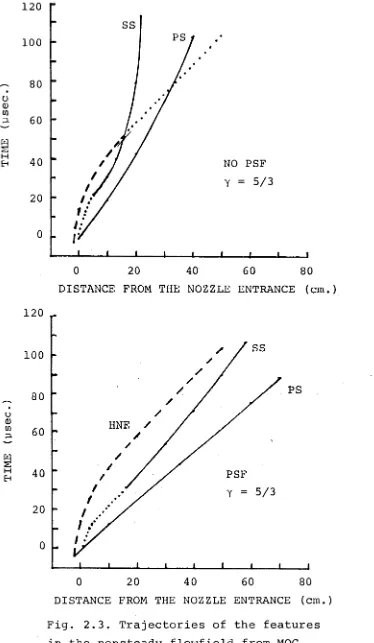
Method of characteristics calculations were carried out for two ratios of specific heats, Y=1.4 and y=5/3. The primary shock speeds for these two cases were those for an initial shock tube pressure of I"Hg of air and of argon respectively. For each y , two calculations were made, one with a prior steady flow and one without.
From the results of these calculations, graphs have been drawn, on the (x,t,) plane, of the trajectories of the primary shock, the secondary shock, and the head of the nonsteady expansion and the left running bicharacteristics which intersect to form the secondary shock. These are
shown in Fig. 2.3.
It can be clearly seen, from the graphs, that the secon dary shock is substantially weakened by the presence of the prior steady flow and remains downstream of the head of the nonsteady expansion until some distance downstream of the test section. When there is no prior steady flow, the sec ondary shock forms early, on the steady (u-a) bicharacter istic originating at the nozzle throat, and then moves upstream, relative to that bicharacteristic curve, and travels far into the steady flow.
The effect of the change in y shows up most strongly in the thickness of the starting shock system. The density
ratio across both shocks decreases with Y and so the rate of growth of the shock system thickness increases with Y .
2.3.3 THE ANALYTIC MODEL.
The analytic model was developed before the M.O.C. programme. A simple version of it was used in conjunction with the early experiments on a nonreflected shock tunnel reported in R. Stalker and N. Mudford (1973).
If, by a simple method, we can find the trajectory of the double shock system and also that of the nonsteady expansion wave (if any), then we will have a fairly complete picture of
the nonsteady flow field, without resort to the time consuming M.O.C. programme.
ASSUMPTION 1 : The flow is approximately one-dimensional. This is the same assumption as made in the MOC calculat
ion and is justified in the same way.
ASSUMPTION 2 : The separation distance betwen the primary and secondary shocks is small compared to the distance over which the nozzle cross-sectional area ratio changes signif
icantly .
This second assumption allows us to assign, to the double shock system, a single point, only, in the (x,t) plane at any one time. The primary and secondary shocks then reside at the same nozzle area ratio and the gas
conditions upstream and downstream of the shock system are those appropriate to that one area ratio. The assumption has the effect that the trajectory calculated is that of the centre of mass of the shock system.
The shock system width has been measured from the inter- ferogrammes (see Chapter 5) for shots with a PSF. The
largest nozzle area ratio change over a typical shock system width is that from A/A =7 to 10. This will not represent a
large change in the gas properties on either side of the
shock system compared with those, say, at A/A =8.5. At other stations in the nozzle, the A / A fc gradient with x is much
smaller.
ASSUMPTION 3 : The gas ahead of the primary shock has neglig ible momentum compared to that imparted to it by the primary shock.
The speed of a section of gas in the PSF is, roughly, 10% of the post primary shock flow speed. The inclusion of this assumption means that the arrival time of the shock system, at a station, will tend to be overestimated for the cases where a prior steady flow exists.
We now write down the integrated momentum equation for the shock system centre of mass:
rt ft
(z,t) = coordinates of the shock system, on the (x,t) plane, at time t.
u = gas speed immediately upstream of the secondary shock.
0
udm + Ap.Adt
0
ft
dm mass which has passed through secondary shock up until time t.
Ap = static pressure difference across shock system. = (upstream pressure - downstream pressure)
A = nozzle cross-sectional area at x.
P3 (x) gas density ahead of primary shock.
The initial conditions, implicit in the above equation, are (z,t,) = (0,0) and that initially, there is no mass in the shock system. The initial shock system speed was taken to be the steady flow speed at the nozzle throat.
In speaking of initial conditions, it is appropriate to point out that, although the secondary shock does not form until some distance down the nozzle (see M.O.C. results in F i g . 2.3), the equation above is valid for the mass of gas entrained between the primary shock and the b icharacteristics which eventually intersect to form the secondary shock.
These bicharacteristics originate not far d o wnstream of the t h r o a t .
The first term in equation (2.3.1) above, represents the m o mentum addition to the shock system due to the passage of gas across the secondary shock. The second term represents the integral of the impulse of the pressure differential across the shock system. The remaining terms represent the current mom e n t u m of the system (i.e. at time t ) .
A further assumption is required to find solutions to this equation of motion:
ASSUMPTION 4 : The gas flow conditions upstream of the secondary shock wave can be taken to be those for the steady test gas flow.
Steady test flow conditions will exist upstream of the secondary shock when there is no prior steady flow. However, when prior steady flow exists, there will, in general, be a nonsteady expansion between the secondary shock and the
steady flow. The assertion made in Assumption 4. is that, although the gas conditions at the tail of the nonsteady expansion may be significantly different from those of the steady flow at the same station, their overall effect on the shock system trajectory will be quite similar.
It should be noted here that, because of this last
restrict-ion often had to be applied near the nozzle throat in the cases where a prior steady flow was present. The static
pressure impulse, acting on the small amount of gas entrained in the shock system in this region, predicted a higher than steady flow speed for the system. The application of this restriction would tend to lead to an overestimation of the time of arrival of the shock system at any station.
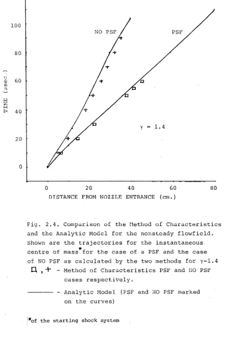
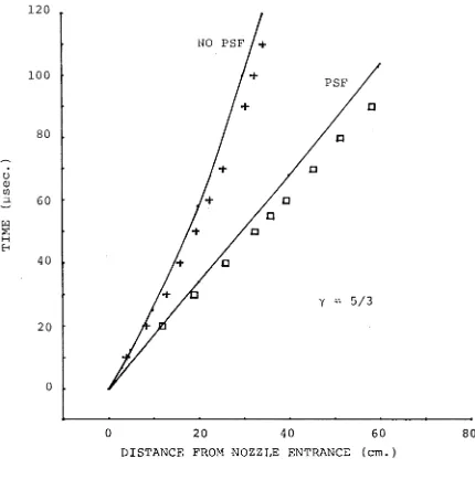
The simplest way to check Assumption 4, and the analytic model in general, is to compare the trajectories of the centre
of mass of the shock system, given by this model, with those predicted by the M.O.C. calculation. The integrals in the equation of motion were evaluated numerically on a Hewlett Packard HP9830a computer, using Simpson's rule. The graphs of the resulting trajectories are shown in Fig. 2.4.
It can be seen from the graphs that, in all cases, there is good agreement between the methods of calculation. In all cases the time of arrival of the shock system at a station is, as expected, overestimated by the analytic model.
2-4 THEORY AND EXPERIMENT
A comparison was made of the shock trajectories predicted by the analytic model and the arrival times of the primary and secondary shocks at a particular nozzle station, in the test section, as measured from the interferogrammes (see Chapter 4, section 4.3.6 for the details of how the inter- ferogrammes were obtained and Chapter 5, section 5.3. for discussion of the measurement of the pressure disturbance trajectories).
The steady flow upstream of the shock system was calcul ated, for input to the analytic model, by the computer
programmes ESTC and NFAPC (see Appendices B and C ) . Chemical dissociation, ionisation, electronic exitation and, in the case of the argon shots,enthalpy loss through radiation in the shock tube, were taken into account in these programmes. For a discussion of the implementation of these programmes, in solving the equations for steady flow, see Chapter 5.
The results of the calculations are shown, with the
15. The analyses presented in the following two sections are due to R. Stalker (1976).
2.5. CONTACT SURFACE MATCHING.
While the contact surface is in the shock tube, the driver and test gas pressure and velocity are matched across
it. When the contact surface passes into the expanding nozzle this matching will not, in general, continue. The test gas flow Mach Number in the shock tube lies between 2 and 4 (see Figs. 5.18 and 5.25). The driver gas Mach Number, on the other hand depends on the shock speed. At
the high shock speeds, the driver gas Mach Number is high. The driver gas then expands to a lower velocity than the test gas and a rarefaction wave travels into both gases. At the lower shock speeds, the driver gas Mach Number is lower. In this case, the driver gas expands to a higher velocity and lower pressure than the test gas. The compress ion wave which subsequently appears in the driver gas is treated as a normal shock for the purposes of performing calculations for this second, more interesting, case.
The normal shock stays close to the contact surface because the mismatch only becomes serious after the driver gas has expanded to a higher Mach Number (>3) in the nozzle. A calculation made for a shock Mach Number of 19 into 10 torr of air with He as driver gas, showed that the pressure
remained matched across the contact surface for a driver gas Mach Number of 1.5 in the shock tube. For a driver gas Mach Number of 1.0, the post shock pressure in the driver gas was higher than the test gas pressure and a compression wave propogated into the test gas. A driver gas Mach Number of 2.25 produced a lower pressure than the test gas at the contact surface and a rarefaction wave propogated into the test gas.
ed. The rarefaction wave, expected in the test gas at lower initial pressures will travel along the steady (u+a) b i
characteristic originating at the nozzle entrance at the time of entry of the contact surface. This bicharacteristic
represents the m i n i m u m pentration of a disturbance from the contact surface mismatch.
The fact that the calculations show that the m a t ched condition is inside the range of experimental shock c o n d i t ions indicates that the disturbance in the test gas will not be a strong disturbance. The i n t e r f e r o g r a m m e s , taken on the flow in the test section, (see Chapter 5) show, in fact, that the contact surface m i s m a t c h disturbance is very small indeed. In m a n y cases, no fringe shift can be detected across the region of the contact surface.
2.6. M I N I M U M N OZZLE LENGTH.
The perfect gas nozzle design programme, described in Chapter 3, was used to calculate the m i n i m u m nozzle lengths for a large range of y and test gas conditions. The results of these calculations showed that the m i n i m u m total nozzle
length, X, could be expressed approximately as X * 1.3 Mt Rt
. . . (2.7-1) . where M T and are the nozzle exit Mach Number and radius.
Neglecting the presence of the starting shock system, the steady flow test time lost due to the presence of the nonsteady expansion wave, is equal to the difference between the arrival times of a steady flow particle trajectory o r i g inating at the nozzle throat at t = 0 and the steady (u-a) bichar a c t e r i s t i c originating at the same point:
At
fX a u(u-a) 0
dx
fX
1 dx M-l u 0
In Fig. 5.8. the trajectories of the steady (u-a) b i characteristics originating at the nozzle throat at the time of primary shock entry are shown with the trajectories of the other important nonsteady flow features for the range of shock conditions.
At can be approximated by
At At s
Cx
dx 0
x r t
m t J2 u u
. . . (2.7-3)
where Atg is the test time lost due to the fact that the flow is supersonic and not hypersonic in the upstream sections of the nozzle. U is the flow speed behind the normal shock -(test section flow speed)/ J2.
expansion of a steady, one - dimensional gas flow with chemical reactions may therefore be used to calculate the flow properties of the region of flow between these two non-steady disturbances. If the ratio of the test gas slug length to nozzle length is such that these two disturbances meet prior to arriving in the test section, then
NFAPC may still be the most reliable available method of predicting the flow properties between the secondary shock and the contact surface because of the importance of chemical reactions in the flow. The ideal tool for the analysis of the nozzle flows would
tube radii, the nozzle inlet radius must be of the order of the shock
tube radius.
This fourth restriction on the nozzle dimensions effectively places an upper limit on the nozzle exit to inlet area ratio. See pp.
16 and 17 for discussion of this restriction. A lower limit for the
nozzle exit to inlet area ratio is set below.
In chapter 5 it is shown that the length of the test gas slug in the apparatus is between 50% and 100% of the nozzle length over the range of gas conditions. In view of this fact it is appropriate to give further consideration to the steadiness or otherwise of the region of the flow between the head of the non-steady expansion (HNE) and the disturbance arising from the entry of the contact surface into the nozzle.
In all the flows considered here the post primary shock flow
r
in the tube is supersonic and a steady expansion of this flow will also, therefore, be supersonic. In the absence of shock waves, a portion of a supersonic flow is affected only by conditions upstream of itself. Consider the test gas flow a short time after the entry of the head of the HNE into the nozzle. The section of flow between the HNE and the shock tube flow must be steady by virtue of the fact that the flow directly upstream of it is steady and that the only change in environment it has encountered since entering the nozzle
is an expansion of the channel walls. By applying this argument to later times in the flow development we may conclude that the flow
3.1. INTRODUCTION.
The requirements and restraints placed on the design of a hypersonic nozzle for the nonreflected shock tunnel are the following:
(i) The nozzle must be axisymmetric.
(ii) The nozzle must be as short as possible.
(iii) The steady flow produced by the nozzle must be both hypersonic (defined as Mach Number ^ 5) and uniform.
The requirement that the nozzle be axisymmetric is made so that the strong boundary layer crossflow effects found in two-dimensional nozzles are avoided. The requirement is consistent with requirements (ii) and (iii) because an axi symmetric nozzle achieves a large area ratio in a short dist ance without requiring a large flow divergence angle anywhere in the flow.
The second requirement arises from the fact that the test time losses due to nonsteady starting and finishing processes increase with increasing nozzle length. Later in this chapter, the minimum possible nozzle lengths will be discussed.
The subject of the third requirement is the desired properties of the steady test section flow. This flow is produced by a steady expansion fron the flow behind the
primary shock in the tube. The Mach Number of the tube flow lies between 2 and 4 and depends on the composition of the test gas and the primary shock speed. Steady nozzle flow calculations made with computer programme NFAPC (see
appendix C) showed that a nozzle area ratio of at least 16 was needed to produce a test section flow with a Mach Number of 5 or more, for all gas conditions.
Having established that the nozzle must be short, axi symmetric, and have an area ratio of 16, we must then decide what the distribution of area ratio along the nozzle axis direction should be so that a uniform test section flow is produced. The choice of this area distribution is the most critical part of the nozzle design. In an axisymmetric nozzle, the strength of an expansion originating at the
.
nozzle is too high, then the streamtubes close to the axis will be forced to diverge to a much greater extent than those near the nozzle wall. The inner and outer streamtubes then come together further downstream and shock waves may form in the flow. Such a flow is said to be overexpanded. A
conical nozzle, cannot, therefore, be used with the non-reflected tunnel because the expansion from the lip of the entrance to a conical nozzle produces an overexpanded flow.
The approach adopted in designing the nozzle was to make a calculation of a flowfield having the desired properties and, then, to take a streamsurface of the flow as the nozzle s h a p e .
3.2. THE NOZZLE DESIGN COMPUTER P R O G R A M M E . 3.2.1. The perfect gas programme.
.if
A computer programme was written by I. Shields to design a suitable nozzle by the method just described. The Method of Characteristics (MOC) for a perfect, inviscid gas'-with a constant y was used to perform the necessary nozzle flowfield c al c u l a t i o n s .
The differential equations governing a steady, s up e r sonic, isentropic axisymmetric flow of a perfect gas are given by Shapiro (1953) in cylindrical coordinates, as:
dr j
-— = tan ( 0 + a) BICHARACTERISTIC (3.2-1) dx
^ jr,l DIRECTIONS
1
u + tana + sina tana sin0 sin ( Q -a)
1
r
dr
dx tan 0
COMPATIBILITY RELATIONS ALONG BICHARACTERISTIC
DIRECTIONS. (3.2-2)
STREAMLINE DIRECTION (3.2-3)
h = a 2 + u 2 (y-1 ) 2
INTEGRATED ENERGY
EQUATION (3.2-4)
S = constant INTEGRATED ENTROPY
EQUATION (3.2-5)
Equations (3.2-4) and (3.2-5) apply along the streamline d i r e c t i o n .
(x,r) coordinates of a point in the physical plane
(distance along symmetry axis, radius from symmetry axis)
flow angle w.r.t. symmetry axis _ l
Mach angle = sin (1/M), where M = Mach N o. = u/a
flow speed
'/* sound speed in the gas = ( 3p/
3p) s
ratio of specific heats
h = specific stagnation enthalpy on a streamline
S = specific entropy (constant along a streamline from eqn (3.2.5) .
The subscripts r and 1 refer to the right and left running bicharacteristics respectively.
The equations (3.2-1) to (3.2-5) are solved, by the M O C , for the unknown quantities (x,r ,u ,6,a ,£)• The problem is simplified by the fact that, because all the streamlines originate in a uniform region, the specific stagnation enthalpy and specific entropy of the gas are the same for all streamlines.
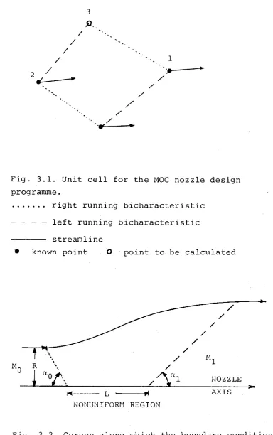
The unit cell for the numerical approximation to the bichar a c t e r i s t i c network is shown in Fig. 3.1. The n u m e r
ical approximation to the differential equations (3.2-1) and (3.2-2) used by Shields are:
r „ - r , (x 3— x1) ( t a n (6 - a) ) ^ 3
(3.2-6a)
r^ - r 2 = (x^ - x 2 ) (tan(6 + a ) ) 2 3
(3.2-6b)
° 3 - (U3 - V
s i n 6 sina\
* (rn - r ,) =0 rsin(6 -aj^
^
r 3 r l... (3.2-7a)
63 - 6 2 cota 2,3
, x , fsinö sincx
)
+ ^ _ n* u 3 ' U 2 + n 2 *3 (r3 V ' 0
The single subscripts refer to the numbered points in the unit cell diagram (Fig. 3.1). The double subscripts signify the arithmetic mean of the quantity between the two points referenced in the subscript. Equations (3.2-6) and (3.2-7) were taken from Shapiro (1953) with a slight modification to the method of obtaining a mean value for the trigonometric functions appearing in the equations. Shields uses the mean of the function values from the two points rather than the function of the mean value of the function arguments at the two points.
In certain circumstances, the coefficients of the last terms in equations (3.2-7) become unstable or indeter minate. For example, if point 1. lies near the symmetry axis where 6 and r are small, then the expression sin6sing
r sin(0-a) in eqn. (3.2-7a) becomes unstable. When this happens,
Shields uses a stable, limiting form of the expression, namely
— ft
lim sin6 sina _ lim -0_ _ '3 r+0 r sin(0-a) - r+0 ~r ~ ~F7
0- +O 0-»O J
along line along line
1- 3 1-3
The other instability allowed for by Shields is that which occurs when a bicaracteristic is nearly parallel to
the x axis. For example, if the bicharacteristic between points 1 and 3 in Fig. 3.1 is nearly parallel to the x axis, then sin(0-a)and (r^-r^ are small and the last term in
equation (3.2-7a) becomes unstable. The following limit is then used in place of this term:
(r3~rl> sin(0-a)
(x3~Xl) cos(0-a)
The replacement expression used if/when the
corres-0
ponding instabilities occur in eqn. (3.2-7b) are _J3 (x3-x )
and
co s (r' + u) respectively. A Mach Number of 20 would be required
before the two types of instability occured simultaneously, so the possibility of this occuring in the nozzle flow can be neglected.
The curves in the (x,r) plane along which the boundary conditions are specified are shown in Fig. 3.2 The first-
N .B . "curve" is used here m
_ . . . •_a rurve. lines are included in the definition of
1 = distance along nozzle axis from the point of the right running bicharacteristic originating at
nozzle throat with the nozzle axis.
2 2
the nozzle entrance to the x axis. Along this curve the specified gas conditions are those existing behind the primary shock in the tube. The second curve is the nozzle axis of symmetry between the two regions of uniform flow. Along this curve a smooth distribution of Mach Angle is
specified. The distribution used is the following:
a = ( ( a Q + ) + ( a Q +0^) cos ( tt (y3 - 2y2 + 2y) ) )/2 ...(3.2-8) where y=l/L, L=length of the nonuniform region on the x
axis (see F i g .3.2) ,0£l ^ L , ,a^=nozzle entrance and exit Mach angles.
The distribution produced the shortest nozzles of a number of "smooth" distributions tried by Shields.
The final boundary curve is the left running bi characteristic originating on the nozzle axis at the end of the nonuniform region. Along this curve the Mach Number is constant and set equal to a chosen nozzle exit Mach Number. The flow angle is zero along this curve and the flow down
stream of it is uniform.
After the characteristics network has been calculated, a stream surface, originating at a specified point along the first flow boundary, is interpolated through the network. This surface is then taken as the nozzle shape.
3.2.2 THE MODIFIED NOZZLE DESIGN PROGRAMME.
The computer programme described above assumed the gas to be a perfect gas with constant y throughout. It is known, however, that strong real gas effects are present in the
test gas flow produced in the shock tunnel apparatus. This knowledge led to concern that the presence of these effects might significantly affect the nozzle shape required to produce an acceptable test section flow.
R. Sedney (1970) has considered the full equations (eqn. nos. (3.2-10) to (3.2-15)) for axisymmetric flow with non-equilibrium chemistry and develops the equations necessary for the solution of the problem by the Method of Characteristics (MOC). However, a large and complex
programme would be necessary to solve these equations.
reactions on the nozzle shape required to produce a test section flow with the desired properties.
The major change made to the perfect gas programme was to replace the perfect gas Mach Number in equations (3.2-1) to (3.2-8) with the Mach Number calculated by the nozzle flow programme NFAPC (see appendix C ). NFAPC solves the problem of a steady one-dimensional nozzle flow, with non equilibrium, frozen or equilibrium chemistry, passing through a given crosssectional area ratio distribution.
The gas flow properties are calculated by NFAPC at discrete, closely spaced stations along the nozzle axis. The sound speed, on which NFAPC bases its Mach Number, is calculated by taking the pressure and density at adjacent nozzle
stations and forming the following ratio:
a is the NFAPC sound speed. Subscripts 1 and 2 refer to the two nozzle stations.
There are two well defined sound speeds for a flow with chemical nonequilibrium:the frozen and the equilibrium sound speeds. The frozen sound speed is defined by
2
af = ^ ^ S = constant, c^ = constant, i=l,...;N The equilibrium sound speed is defined by
ae E (3p/3p ) s _ constant, c^ = c^ , i=l,.../N. where S = specific entropy, c^ = specific molar concentration of species i, (moles of i)/(gm. of mixture), c^e = equilibrium c^, N = number of species present in flow.
Clearly, the NFAPC sound speed is not an approximation to either of these sound speeds because, between nozzle stations 1 and 2, the specific entropy is allowed to vary and the flow chemistry is out of equilibrium but not frozen. The NFAPC "nonequilibrium sound speed", however, expresses
the response of the nonequilibrium gas flow to a change in pressure. In this capacity, it was employed in the modified nozzle design programme in the form of the NFAPC "non
equilibrium Mach Number".
2 4.
initial gas conditions of interest through an area ratio distribution similar to that of the expected, final nozzle shape. The Mach Number at each station was then plotted against the flow speed over the desired exit to throat area ratio range and a polynomial, of up to 6th order, was fitted to the resulting curve. The polynomial was used by the
nozzle design programme whenever it was necessary to obtain the Mach Number from the flow speed or vice versa. In the original perfect gas programme, the energy conservation equation, eqn. (3.2-4) was used for this purpose. The
introduction of the M^ vs. u polynomial can therefore be looked upon as a way of varying the ratio of specific heats, Y in order to approximate the real gas flow more closely
than possible with the constant y model.
Justification for the use of the NFAPC Mach Number is found from a consideration of the flow equations for axisymmetric flow with chemical nonequilibrium presented by Sedney (1970) written in the natural coordinates s,n= distance along streamline, distance normal to streamline:
1
+ I
l£ + Ü J . + sin. 9 = 0 CONTINUITY (3.2-10)u 9s p 3s 3n r
P MOMENTUM IN
s DIRECTION (3.2-13)
pu2 3 6 , 9_P
3 s 3n 0 MOMENTUM IN
n DIRECTION (3.2-12)
h + INTEGRATED ENERGY
EQUATION (3.2-13)
pu 3Ci 3 s
o k, i=l, . . . , N SPECIES PRODUCTION
RATE (3.2-14)
TdS = dh - — dp - l
p i=! y i w i dci
0 GIBBS EQUATION
where p = mass density p = pressure u = flow speed
0 = flow angle
h = specific enthalpy
r = radius from axis of symmetry
c^ = (moles of species i)/(gm. of gas mixture) ,i = l , N N = number of species present in the flow
= rate of production of species i T = temperature
M^ = chemical potential of species i VA = molecular w eight of species i
The NFAPC speed of sound is introduced into the set of equations through the relation:
1 9_p
p 9s 1 P
1 9P - 1 9P
2 2
pa 9s pa.T 9s
n N
... (3.2-16)
This relation defines the "nonequilibrium speed of sound", a . The subscript n denotes that the derivative is taken allowing the chemical reactions to proceed at their n o n equilibrium rates. Equ a t i o n (3.2-9) shows that the NFAPC speed of sound is an a pproximation to the nonequil i b r i u m speed of sound.
The corresponding expression used by Sedney is: 1 ^p
p 9 s
-1
ph
ph -1
P 9p
9c c . 9 s
l
1 9p _ 1 a? 9s h i
f P
Ih,
9c i9 s
(3.2-17)
where subscripts denote partial derivatives of h = h(p,p,c^) with respect to the variable men t i o n e d in the subscript. Sedney's equation is obtained by taking the partial d er i v a t ive of the integrated energy equation along the streamline d i r e c t i o n .
Substituting equation (3.2-16) into equation (3.2-11) and then substituting the result into equation (3.2-10) we have
(M^ - 1) 9u 90 sin0
JO---= 0 ...(3.2-18)
where is the M ach Number based on the nonequilibrium speed of sound.
Substituting the differential form of the energy
equation (3.2-13) into the Gibbs Equation (3.2-15) and then taking partial derivatives along the streamline direction and normal to the streamline direction, we have:
T
3S 3c i
3s + l ^i3s l
0 ... (3.2-19)
T
as
, 1 3u 30 , 1 v 3ci~ 2 — + --- t l l ---u 3n u 3n 3s u i dn
0
...(3.2-20)
In obtaining these equations the fact that the stagnation enthalpy is constant along a streamline and the same for all streamlines has been used. Also equation (3.2-11) was used to eliminate the derivatives of u and p in equation
(3.2-19) and equation (3.2-12) was used to eliminate the p derivatives for equation (3.2-20).
Now define the directional derivatives
3_
3C c o s (a )n 3_
sin(a ) n
3_
3n . . . (3.2-21)
3_
3n cos (a )n tt3 s— sin(a )n
3_
3n
. . . (3.2-22)
where a is the Mach Angle based on the nonequilibrium n
Equations (3.2-21) and (3.2-22) are the d i r e c t i o n al derivatives in directions ± a to the streamline direction.
n
At this point we take the following linear combinations of the equations
cosa
s i n a n * (3.2-18) - — ~ - *(3.2-20) +
sina cot^a
n n
* (3.2-19)
This gives the equations
cota
n 3u 36 sina sin6 n , cota n
u H + 3C r + 2
u [t h
cotan 3u 36 sina sin6 cota r 3rT
n
i n m 9 _ S
3n
u 3n r + 2
u
3c £
3c 3n
0 (3.2-23)
0 (3.2-24)
The question now is whether the £ and n directions, as defi n e d in equations (3.2-21) and (3.2-22) above, can be c o n
sidered to be characteristic directions for the flow e q u a t ions and, therefore, whether equations (3.2-23) and (3.2-24) can be used as compatibility relations, along those d i r e c t ions, to solve the flow problem.
The definition of a "characteristic direction" used by Sedney is one taken from Courant and Hilbert (1962):
"Along a characteristic curve the differential equation (or for systems a linear combination of the equations) r e p resents an interior differential equation".
With respect to a curve, an interior differential
equation is one in which the directional derivatives are all taken along the curve direction. Alternatively, it is one
in whi c h the values of the derivatives of a function, f, on the curve, depend only on the values of f on the curve. The discovery of these curves along which the governing d i f f e r ential equations take a simple, easily integrable form is the basis of the MOC solution.
Comparison of equations (3.2-16) and (3.2-17) shows that the nonequil i b r i u m sound speed can be written as
d£ dp
ph -1
P +
h i£ p 3 s
y h io.
L c . 1
l
-1
This equation shows that a^ has some dependence on the pressure gradient in the streamline direction. This dependence is, however, known to be extremely weak. The pressure gradient in the streamline direction in the one dimensional flow calculated by NFAPC can be altered by increasing or decreasing the nozzle length while holding 1 the nozzle area ratio constant. Runs of NFAPC with nozzles of various lengths show the nonequilibrium sound speed to be unaffected by a doubling or halving of the nozzle length.
The length and shape of the nozzle used for the nozzle design runs of NFAPC was similar to that of the final nozzle design. The pressure gradients in the flow calculated by NFAPC were therefore similar to those in the final nozzle. The nonequilibrium sound speed at a point can therefore be considered as a function of the flow properties at that point for the purposes of the nozzle design. The £ and n directions are then bicharacteristic directions and the equations (3.2-23) and (3,2-24)_are■the compatibility relat ions for those directions.
The difference in form between equations (3.2-23) and (3.2-24) and the corresponding equations for a perfect gas is the existence of the final terms in equations (3.2-23) and (3.2-24). If the final term in each equation can be
shown to be small compared to any other term in each equation, then the final term can be neglected and the perfect gas form of the equations can be used for the MOC calculations.
The procedure employed to assess the relative magnitude of the terms in equations (3.2-23) and (3.2-24) was as