This is a repository copy of Learning with precise spike times : a new decoding algorithm
for liquid state machines.
White Rose Research Online URL for this paper:
http://eprints.whiterose.ac.uk/150753/
Version: Accepted Version
Article:
Florescu, D. and Coca, D. orcid.org/0000-0003-2878-2422 (2019) Learning with precise
spike times : a new decoding algorithm for liquid state machines. Neural Computation, 31
(9). pp. 1825-1852. ISSN 0899-7667
https://doi.org/10.1162/neco_a_01218
© 2019 Massachusetts Institute of Technology. This is an author-produced version of a
paper subsequently published in Neural Computation. Uploaded in accordance with the
publisher's self-archiving policy.
[email protected] https://eprints.whiterose.ac.uk/ Reuse
Items deposited in White Rose Research Online are protected by copyright, with all rights reserved unless indicated otherwise. They may be downloaded and/or printed for private study, or other acts as permitted by national copyright laws. The publisher or other rights holders may allow further reproduction and re-use of the full text version. This is indicated by the licence information on the White Rose Research Online record for the item.
Takedown
If you consider content in White Rose Research Online to be in breach of UK law, please notify us by
1
Learning with precise spike times: A new decoding algorithm for liquid state
ma-chines
Dorian Florescu, Daniel Coca∗
Department of Automatic Control and Systems Engineering, The University of Sheffield,
Sheffield, S1 3JD, UK.
Keywords:spiking neural network, temporal coding, integrate-and-fire neuron,
liq-uid state machine
Abstract
There is extensive evidence that biological neural networks encode information in
the precise timing of the spikes generated and transmitted by neurons, which offers
several advantages over rate-based codes. Here we adopt a vector space formulation
of spike train sequences and introduce a new liquid state machine (LSM) network
ar-chitecture and a new forward orthogonal regression algorithm to learn an input-output
spike timing to select the presynaptic neurons relevant to each learning task. We show
that using precise spike timing to train the LSM and selecting the Readout presynaptic
neurons leads to a significant increase in performance on binary classification tasks, in
decoding neural activity from multielectrode array recordings, as well as in a speech
recognition task, compared with what is achieved using the standard architecture and
training methods.
1 Introduction
It is generally accepted that neurons in the brain encode information not only in their
average firing rates - rate coding - but also in the precise timing of spikes - temporal
coding (Hirata et al., 2008). The importance of the precise spike timing information has
been documented in many studies (Srivastava et al., 2017; Memmesheimer et al., 2014;
Kayser et al., 2009; Jones et al., 2004; Gollisch & Meister, 2008; Riehle, 1997). Seth
(2015) has argued that the two encoding schemes are in fact complementary.
Neuronal coding is reproducible with a precision of a millisecond (Mainen &
Se-jnowski, 1995; Izhikevich, 2006). It has been argued that codes that utilise spike timing
make better use of the capacity of neural connections than those relying on rate codes
(Mainen & Sejnowski, 1995) and that it allows processing information on much shorter
time scales allowing to track rapidly changing signals (Gardner & Grüning, 2016).
There is also evidence that during perceptual decisions, learning and behaviour can
be driven by a small number of neurons that are trained to read out and interpret very
sparse, precisely timed action potentials (Huber et al., 2008; Houweling & Brecht, 2008;
In recent years, a lot of research effort has been expanded to establish a sound
the-oretical basis for encoding and decoding using the precise timing of the spikes rather
than spike-count rates (Lazar & Pnevmatikakis, 2008; Florescu & Coca, 2015; Lazar &
Slutskiy, 2015; Florescu, 2017; Florescu & Coca, 2018). A range of supervised
learn-ing approaches that utilise temporal codlearn-ing schemes have been developed for recurrent
spiking neural networks (SNNs) with feedforward and feedback connections (Gardner
& Grüning, 2016; Gütig, 2014). Some of the popular SNN training algorithms using
temporal coding are based on gradient descent (Bohte et al., 2002; Xu et al., 2013;
Flo-rian, 2012; Pfister et al., 2006) or on spike timing dependent plasticity (Pfister et al.,
2006; Florian, 2007; Izhikevich, 2007; Ponulak & Kasinski, 2010).
Liquid state machines (LSM) (Maass et al., 2002) are a class of recurrent SNNs
that consist of a fixed high-dimensional dynamical network of biologically-realistic
synapses and spiking neurons that remain unchanged during training, known as
reser-voir or ’Liquid’, followed by a memoryless output or ’Readout’ unit with adjustable
synaptic weights. The Readout typically combines in a linear fashion the outputs of
all the neurons in the Liquid. The LSM model can be viewed as a nonlinear
dynam-ical system where the state vector comprises the states of all neurons in the Liquid,
evolving in time according to the internal dynamics and external driving inputs, and the
static Readout defines the relationship between the state vector and output (Maass et al.,
2002).
The LSMs belong to the general class of reservoir computing approaches, which,
compared with high-dimensional recurrent neural networks, have more biologically
the connections to the Readout unit (Lukosevicius & Jaeger, 2009).
The reservoir computing approaches also include non-spiking models, as the Echo
State Networks (ESNs) (Jaeger, 2001). However, the LSMs are more biologically
real-istic than ESNs and thus better suited for reproducing the computational properties of
biological neural circuits.
The LSM Readout is typically trained by performing linear regression using the
spike train outputs of the Liquid converted to continuous signals with exponential filters
(Maass et al., 2002). Other proposed LSM models have feedback connections from the
Readout, and are trained with recursive least squares using the filtered outputs of the
Liquid (Nicola & Clopath, 2017). This leads to losing the information of the exact
spike times generated by the Liquid neurons. The current training methods for LSMs
learn target outputs using measurements from all the presynaptic neurons (Maass et al.,
2002; Verstraeten et al., 2005) . Numerically, this model contains a large number of
parameters which can lead to overfitting for large neural circuits. Moreover, it is known
that only a relatively small number of cortical neurons project to different areas of the
central nervous system (Häusler & Maass , 2007; Thomson et al., 2002).
In the case of ESNs, Dolinský et al. (2017) used orthogonal forward regression
(OFR) to identify the contribution of each individual neuron to the response variable,
and concluded that a small number of presynaptic neurons are enough to achieve
accu-rate results.
Here we propose a new liquid state machine (LSM) architecture, and a new training
algorithm that outperforms the standard methods (Maass et al., 2002; Verstraeten et al.,
spike time based Readout. The new algorithm, called OFR with Spike Trains (OFRST),
identifies the best synaptic connectivity for the Readout unit of the LSM. The learning
algorithm relies on a distance metric between two spike trains that are elements of an
inner product vector space (Carnell & Richardson, 2005).
Theoretical results demonstrate that the proposed architecture can learn any
contin-uous target output by mapping it onto a unique target spike train sequence. We prove
that the proposed LSM architecture achieves higher accuracy in training compared with
the standard methods.
Numerical simulations are given to show the performance of the proposed method
compared to the standard methods for binary and multi-label input classification tasks.
Additional numerical examples are used to show separately the benefit of selecting
the Readout connectivity using OFR and computing with precise spike times. The
advantage of the proposed method is also demonstrated for two problems involving
real world data. First we consider the problem of classifying the movement direction
of drifting sinusoidal gratings using visually evoked multi-array recordings from the
primary visual cortex of the monkey. Second, we test our method against the standard
methods on a problem of speech recognition.
The paper is structured as follows. Section 2 introduces the standard architecture
and method for training an LSM. Section 3 presents the proposed approach. Numerical
2 The Standard LSM Architecture and Training Method
The spike train inputs and outputs of the LSM are elements of spaceS0satisfying
S0 =
s|s={tk}Pk=1, tk+1 > tk≥0,∀k = 1, . . . , P −1
The Liquid is modelled by an operator L, which maps the vector of input spike
trains sin into a vector of continuous functions x(t), also known as the state of the
Liquid. The Readout is modelled by operator
R
, which mapsx(t)into the continuousscalar functiony(t), which denotes the LSM output. The functiony(t)satisfies (Maass
et al., 2002)
y(t) =
R
Lsin,wheresin =
sin
1 , . . . , sinNin
, sin
k =
n
tin
k,1, . . . , tink,Pin k
o
, L : [S0]Nin
→ [L2(R)]N,
R
:[L2(R)]N → L2(R), where N
in and N denote the number of inputs and number of
neurons in the SNN, respectively, Pin
k denotes the number of spikes in input k, and
x(t) = (Lsin) (t).
The Liquid is represented as the composition of two mathematical operators L =
F LSN N, where LSN N : [S0]Nin
→ [S0]N models a generic SNN and F : [S0]N →
[L2(R)]N,Fs= [
F
s1,
F
s2, . . . ,F
sN],∀s∈[S0]N,s= [s1, . . . , sN]models a pool oflinear filters
F
sn= PnX
k=1
e−
t−tnk τs ·1[tn
k,∞)(t), (1)
wherePndenotes the number of spikes insn,1[tn
k,∞)denotes the characteristic function
of interval[tn
k,∞), andτsdenotes the time constant of the filter.
Maass et al. (2002) demonstrated that this model has, under idealised conditions,
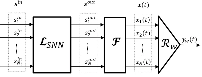
Figure 1.
Figure 1: Block diagram of the standard architecture used for training LSMs. It consists
of three blocks connected in series: the Liquid LSN N, the pool of filters F and the
readout
R
w.Remark 1.Throughout the paper, it will be assumed thatsout
k 6=soutl ,∀k, l∈ {1, . . . , N},
k6=l. In a practical scenario it is very unlikely that two neurons will generate two
iden-tical spike trains simultaneously. However, if this happens to be true, only the distinct
outputs will be used for training.
The most common Readout is the linear unit
R
Wx(t) = PNn=1wnxn(t), where
W = [w1, . . . , wN]andx(t) = [x1(t), . . . , xN(t)]. This Readout was shown to classify
time-varying inputs with the same power as complex non-linear Readouts, given a large
enough Liquid (Häusler et al., 2002). A typical way to train the Readout is by tuning
the weights using the least squares (LS) algorithm
wopt =argmin
w k
y∗−ywkL2, (2)
wherey∗ ∈L2(R)denotes the target output function,k · k
L2 denotes the standard norm
inL2(R)andy
In practice, the continuous state of the liquidx(t)is sampled uniformly with period
∆T > 0. The functionx(t) = [
F
sout1 ,
F
sout2 , . . . ,F
soutN ]is not continuous in amath-ematical sense at points {tn
k}Pk=1n , n = 1, . . . , N, due to the expression of operator
F
(1). Therefore, for any sequence of spike trains{sout
1 , . . . , soutN }, x(t)in not
bandlim-ited. This can also be explained by viewing the values of operator
F
as the output of anexponential filter with impulse responseh(t) = e−τst , given a train of Dirac delta pulses
PPn
k=1δ(t−tnk). Given that the filter is not ideal, its output has arbitrarily large frequency
components, and thus the samples{x(kT)}are affected by aliasing, due to Shannon’s
law. This leads to computing weightswoptthat are deviated form the theoretical optimal
values, as well as an imprecise final output predictionywopt(t).
Moreover, in practice not all synaptic connections of the Readout are relevant to a
particular task, so that training the weights of all possible connections from the Liquid
neurons to the Readout can easily lead to overfitting.
There are a few variations of LS that introduce an additional parameter, also known
as hyperparameter, in order to control the effective complexity of the model and to
re-duce overfitting. Some of the standard methods doing this are LS withL2regularization,
or ridge regression (RR), LS withL1 regularization, or lasso, and early stopping (ES).
The regularization parameter for RR and lasso, and the number of iterations for ES
are typically tuned to minimise the prediction error on the validation dataset (Bishop,
2006). These methods can lead to a Readout with smaller weights, or fewer presynaptic
connections to the Liquid.
However, computing the Readout weights with RR, lasso or ES is affected by
leads to Readout presynaptic connections to neurons that are less relevant for the
com-puting task. Furthermore, the output spikes of a biological neural network do not lie on
a grid of uniformly spaced time points, and therefore are not directly compatible with
the training methods above.
3 A New LSM Training Approach using Precise Times
3.1 The Carnell-Richardson Spike Train Space
The spaceS0is not a linear space because it does not allow any operations between spike
trains. To overcome this problem, this space is extended to the Carnell-Richardson spike
train space (Carnell & Richardson, 2005)
S=ns={(ak, tk)}P
k=1, P ≥1, tk, ak∈R, tk =6 tl,∀k, l∈ {1, . . . , P}, k6=l
o
.
Carnell & Richardson (2005) have proven thatS is an inner product space, where
the vector sum, scalar multiplication and inner product of two spike trains s1, s2 ∈ S
are defined as
s1+s2 ={(a1k, t1k)}Mk=11 ∪ {(a2k, t2k)}Mk=12 ,
α·s={(α·ak, tk)}Mk=1,∀α∈R,
hs1, s2iS=
k1=M1,k2=M2 X
k1=1,k2=1
a1k1a2k2 ·e−
|t1 k1−t2k2|
τs ,
whereτs > 0is a scaling factor. The inner producth·,·iS generates a normk · kS
sat-isfyingkskS =
p
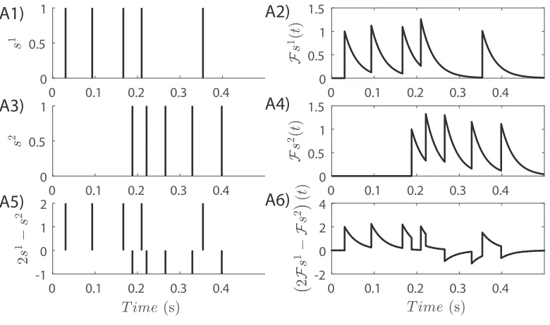
hs, siS,∀s ∈ S. Figure 2 illustrates an example of a linear operation
between two randomly generated spike trainss1, s2 ∈S, presented comparatively with
0 0.1 0.2 0.3 0.4 0
0.5 1
0 0.1 0.2 0.3 0.4
0 0.5 1 1.5
0 0.1 0.2 0.3 0.4
0 0.5 1
0 0.1 0.2 0.3 0.4
0 0.5 1 1.5
0 0.1 0.2 0.3 0.4
-1 0 1 2
0 0.1 0.2 0.3 0.4
[image:11.612.102.492.111.342.2]-2 0 2 4
A1)
A3)
A5)
A2)
A4)
A6)
Figure 2: An example of a linear operation inS. Two spike trainss1,s2 ∈ S, and their
corresponding elements
F
s1,F
s2 ∈ L2(R), are generated in time interval [0,0.5 s](A1-4). The equivalent linear operations in the two spaces2s1 −s2 and2
F
s1 −F
s2are depicted in (A5-6).
A spike trains0 ={tk}Pk=1 ∈S0, as defined by the standard method, can be mapped
uniquely onto an elements ∈ S, such thats = {(1, tk)}P
k=1. Maass et al. (2002) have
defined a metricdonS0
d(s1, s2) =
Z
R
[(
F
s1) (t)−(F
s2) (t)]2dt1/2
,
where
F
: S0 → L2(R),F
s = PPk=1e −t−τstk
·1[tn
k,∞)(t)denotes the output of a linear
filter with exponential decay and time constantτs,given spiking inputs.The normk·kS
relates to metricdas followsks1−s2k2S = 2·d(s1, s2)2,∀s1, s2 ∈ S0.However, in a
sampling time∆T.Then the following holds
lim
∆T→0d∆T(s1, s2) =
1
√
2ks1−s2kS.
In order to show the disadvantage in computing d∆T, we generated two random
spike trains s1 and s2 with 100 spike times each. We then computed ks1 −s2kS and
d∆T(s1, s2) for 100 values of ∆T on [1 ms,100 ms], and τs = 30 ms. The results,
depicted in Figure 3, show that the values ofd∆T(s1, s2)/
√
2oscillate aroundks1−s2kS
as∆T →0.However, the computing time ford∆T increases exponentially with1/∆T.
Thus, at the sampling interval of 2 ms, which is used to simulate the LSM, the spike
based metric results in a similar value to the standard metric, but runs three times faster.
0 0.2 0.4 0.6 0.8 1 0
0.5 1
0 0.2 0.4 0.6 0.8 1 0
0.5 1
100 101 102
1.5 2 2.5
100 101 102
10-2 100 102
A1)
A2)
[image:12.612.128.485.390.540.2]A3)
A4)
Figure 3: Comparison between the Carnell-Richardson spike train distanceks1 −s2kS
and the standard metricd∆T(s1−s2): two randomly generated spike trainss1, s2(A1,2)
3.2 The Proposed LSM Architecture and Training Method
We propose a new spike time based Readout architecture, which does not require the
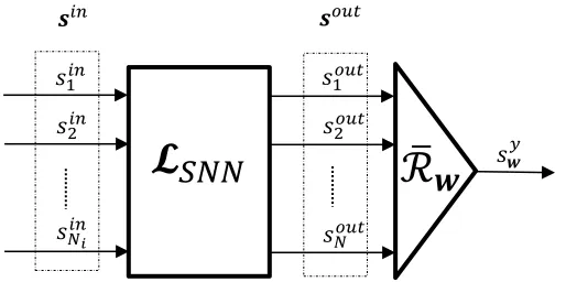
[image:13.612.180.437.181.314.2]bank of filtersF (Figure 4).
Figure 4: Block diagram of the proposed architecture used for training LSMs ,
consist-ing of two blocks connected in series: the LiquidLSN N and the proposed spike based
Readout
R
¯w.The Readout
R
¯wis defined using the operations inSas¯
R
wsout =Pout n
X
n=1
wnsoutn =syw.
Letsy∗ be a target spike train. Then the optimalwin the least squares sense is
¯
wopt =argmin
w k
sy∗−sywkS,
wherek · kSdenotes the standard norm inS.
The proposed architecture can be extended to learn continuous target signals. To this
end, the following results demonstrate that any continuous target functiony∗ ∈ L2(R)
Theorem 1. LetSoutdenote the subset of Sgenerated by the outputs of the SNN, such
thatSout =span{sout
1 , . . . , soutN } ⊂S.Let
F
:Sout →L2(R)be an operator defined byF
s= PX
k=1
ake−
t−tk
τs ·1[t
k,∞)(t),∀s∈S
out, s=
{(ak, tk)}Pk=1. (3)
Moreover, letFSout denote the subset ofL2(R)generated by the filtered outputs of
the SNN, such that FSout = span{
F
sout1 , . . . ,
F
soutN }.Then the following mapping iswell defined
M
:L2(R)→Sout,M
(y) =F
−1P
FSout(y),∀y∈L2(R), (4)where
P
denotes the projection operator.Proof. See Appendix 1.
Theorem 1 defines a mapping that allows converting any continuous target output
functiony∗(t)into a unique target output spike train sy∗.The operator
F
in (3) is theextension of the filtering operator in (1) to the more general spaceS. The following
result assesses the prediction accuracy of the proposed method relative to the standard
method for continuous target functions.
Theorem 2. Lety∗ ∈ L2(R) and letw
opt be the vector of weights computed for the
standard architecture, such thatwopt =argmin
w k
y∗ −
R
wFsoutkL2. It follows that
wopt =argmin
w k
sy∗−
R
¯wsoutkS = ¯wopt,wheresy∗ =
M
(y∗),M
(y∗) =F
−1P
FSout(y∗),
P
denotes the projection operator andFSout =span{
F
sout1 , . . . ,
F
soutN }.Corollary 1. Theorem 2 proves that the proposed methodology achieves, in theory, the
same accuracy as the state-of-the-art method when learning continuous target signals.
In practice, however, the accuracy of the standard method is lower because it is affected
by the approximation error introduced when calculatingwoptandywopt(t)from uniform
samples, which doesn’t affect the proposed method.
3.3 The Orthogonal Forward Regression with Spike Trains (OFRST) Algorithm
The optimisation problem addressed by the proposed method is to learn a continuous
target outputy∗(t)given a SNN of sizeN. Let{sout
k }Nk=1denote the outputs of the SNN
in response to stimuli{sin k }
Nin
k=1. Computing the optimalwopt in the least squares sense
(Maass et al., 2002) leads to many non zero weights that are not particularly relevant for
the learning task and overfit the data. Furthermore, the standard methods that address
this problem using regularization or early stopping lead to weights that are deviated
from the theoretical optimal weights as a result of the approximation error.
Theorem 1 demonstrates that the problem addressed here can be reduced to learning
a target spike trainsy∗, uniquely derived from the continuous targety∗(t).This leads to
a more precise estimation of weights wopt (Theorem 2). Here we introduce a greedy
selection algorithm for the spike trains that are most relevant for the learning task, called
Orthogonal Forward Regression with Spike Trains (OFRST). The OFRST algorithm
is inspired by the orthogonal forward regression (OFR) for finite dimensional spaces
(Chen et al., 1989). The remaining part of this section will first present the classical
OFR and then the proposed OFRST algorithm.
a subset{xℓ1. . . , xℓp}and an estimate of the parameters{wℓ1, . . . , wℓp}that fits the data
y∗.
At the first stage, y∗ is projected onto basis vectors {x
1, . . . , xN}. Then the
error-reduction-ratio (ERR) is calculated for each vector, defined as
ERR(1)k = hxk, y
∗i2
kxkk2 · ky∗k2
.
The magnitude ofERR(1)k represents the proportion of the dependant variable variance
explained byxk.A geometrical interpretation of the ERR is depicted in Figure 5 for the
simplified case wherexk ∈ R2, k = 1,2,andy∗ ∈ R2.The maximum ERR, computed
as ERR1 = ERRℓ(1)1 = maxk=1,...,N{ERR
(1)
k }, leads to the selection ofx⊥1 = xℓ1 as
[image:16.612.184.425.384.544.2]the basis for the one-dimensional spaceE1.
Figure 5: Geometrical interpretation of OFR for the simplified two-dimensional
sce-nario. In this caseERR(1)1 > ERR2(1) implies that x1 explains a larger proportion of
the variance of target outputy∗.
At the second stage, the rest of the vectors{xi}i=1,...,N,i6=ℓ1 are projected, through
Subsequently, the vector xℓ2 is selected and orthogonalised with the Gram-Schmidt
procedure to computex⊥
2. The vectorsx⊥1 andx⊥2 form the basis for two-dimensional
spaceE2.Similarly, at stage numberp, the vectorxℓpis selected, which is used to define
thep-dimensional spaceEp with orthogonal basis{x⊥i }i=1...,p. The detailed algorithm
is given in Appendix 2.
The OFRST algorithm closely follows the steps of the OFR algorithm, implemented
for the Carnell-Richardson spike train spaceS. Initially, lets⊥(1)
k = soutk ∈ S,∀k =
1, . . . , N, be the complete set of SNN outputs. The most significant spike trainsout ℓ1 is
defined as the one that maximisesERR(1)k , whereERR(ki)denotes the
error-reduction-ratio (ERR) of termkat iterationi, defined as
ERRk(i) =
D
s⊥(k i), sy∗E2
S
ks⊥(k i)k2
S· ksy∗k2S
.
Subsequently, the set{s⊥(2)k }N
k=1,k6=ℓ1 is computed by orthogonalising the remaining
output spike trains againstsout
ℓ1 using the Gram-Schmitt routine.
The process continues iteratively. At every iterationi, the algorithm selects the next
most significant spike train sout
ℓi such thatℓi = argmax
k
ERR(ki), and generates the
set{sout
ℓ1 ,· · · , s
out
ℓi }of significant SNN outputs and the corresponding vector of weights
w(p). Subsequently, the set{s⊥(i)
k }Nk=1,k6=ℓ1,...,ℓi is computed from the remaining spike
trains through orthogonalisation. The process continues untilp=N. The final number
of presynaptic neurons is selected as the smallestpthat leads to the maximum prediction
4 Numerical examples
The proposed new Readout and associated training algorithm is evaluated in comparison
with the standard architecture trained with LS, RR, lasso and ES.
Additional numerical examples show the advantage of using a spike based Readout
and the advantage of selecting the Readout presynaptic neurons using OFRST. The
benefit of the proposed method is also demonstrated for two additional examples with
real world data. First, OFRST is compared against the standard methods for a
multi-label classification problem using multi-array recordings from the primary visual cortex
of the monkey. Second, the advantage of the proposed method on a speech recognition
task is shown using data from the TI-46 corpus database of spoken digits.
The LSM was simulated using the toolbox described in (Natschläger et al., 2003).
The Liquid consists of leaky integrate-and-fire neurons,20% of which were randomly
selected to be inhibitory (Maass et al., 2002). The connection probability between
neu-ronsaandbis defined asC·e−(D(a,b)/L)2, whereD(a, b)denotes the Euclidian distance
between the neurons, L = 2is a parameter that controls the average number of
con-nections and the average distance between neurons, andC, depending on whether the
neurons are excitatory (E) or inhibitory (I), is0.3(EE),0.2(EI),0.4(IE),0.1(II). The
synaptic transmission is given by the dynamic model proposed in (Markram, Wang &
Tsodyks, 1998). The input is injected into30%randomly chosen neurons in the Liquid
with an input gain of0.1. For the standard Readout architecture, the time constant of the
exponential filters isτs = 30ms. The LSM was simulated using the default sampling
8.6 (R2015b)on a3GHz Intel Core i7-5960X 8 core PC workstation.
Example 1. Binary classification - comparison with the standard methods.
This example compares the performance achieved by a standard LSM with the
Readout parameters estimated using the LS, RR, lasso and ES with that of a LSM
com-prising a spike-based Readout trained using the proposed OFRST method. The LSM
consists of240neurons spatially organised as a lattice with dimensions15x4x4.
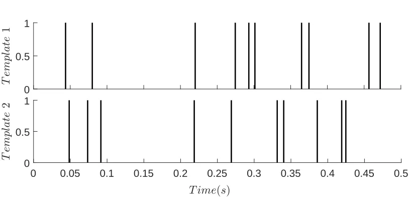
The task is to discriminate between two spike train templates using the SNN
re-sponses. The templates are two instances of a Poisson point process with rate 20Hz,
depicted in Figure 6.
0 0.5 1
0 0.05 0.1 0.15 0.2 0.25 0.3 0.35 0.4 0.45 0.5 0
[image:19.612.105.512.387.583.2]0.5 1
Figure 6: The input templates used for classification, generated as Poisson spike trains
with frequency20Hz over time interval[0,0.5s].
The inputs are generated in time interval[0,0.5s]by jittering one of the two
and standard deviation6 ms. A number of 100 jittered templates were generated for
each class, of which50were used for training and50for validation. The two classes
of inputs are assigned the target output labels y(t) = 1 (template 1) and y(t) = −1
(template2),t ∈[0,0.5s].
The input-output mappings are learned with the LSM by estimating the standard
Readout parameters using LS, RR, lasso and ES, where the sampling time is∆T = 20
ms (Maass et al., 2002; Verstraeten et al., 2005). Subsequently, the spike time based
Readout is trained using OFRST. The regularization parameter for RR and lasso, the
number of steps for ES and the numberpof presynaptic neurons for OFRST are
com-puted using a line search that maximises the prediction accuracy on the validation
dataset.
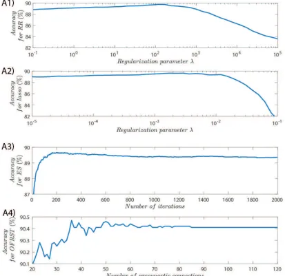
The classification accuracies for RR, lasso, ES and OFRST were evaluated as a
function of the hyperparameter and averaged over100 trials. Each trial consisted in a
different Liquid and a different instance of jitter applied to the input. The results are
depicted in Figure 7.
In the case of the OFRST algorithm the results show that, on average, the
accu-racy drops when using more than 36Readout presynaptic connections, or equivalently
training for more than36iterations. This suggests that, on average, more than30
Read-out presynaptic connections lead to overfitting the data. This result mimics what has
been observed experimentally in cortical circuits, where only a small number of
cor-tical neurons project to different areas of the central nervous system (Thomson et al.,
2002; Häusler & Maass , 2007).
Figure 7: Binary classification with RR (A1), Lasso (A2), ES (A3), and OFRST (A4),
as a function of the regularization parameter. The average accuracies were computed
each simulation trial. The classification accuracies achieved by all the methods over
100 trials are given in Table 1. The results show that, on average, OFRST has the
[image:22.612.110.504.276.375.2]highest accuracy from all methods while using the smallest number of synapses.
Table 1: Binary classification results using pools of240neurons. Comparison between
least squares, ridge regression, lasso and early stopping, implemented for the standard
Readout, and the proposed OFRST method for the spike based Readout. The mean (±
standard deviation) is computed for each method over100trials.
Training method Total number of Readout connections Accuracy Least squares 56.46 (±20.3) 88.4% (±7.28%)
Ridge regression 56.46 (±20.3) 91.27% (±7.07%)
Lasso 40.32 (±23.07) 91.15% (±6.8%)
Early stopping 56.46 (±20.31) 91.28% (±7.07%)
OFRST 15.05 (±11.03) 92.15%(±6.92%)
Example 2. Binary classification - benefits of learning with exact spike times.
In this example we compare the classification accuracy of the proposed Readout
trained with the OFRST method to that of the standard Readout trained with LS, RR,
lasso, ES and classical OFR (Billings et al., 1989) on the same binary classification task
as in Example 1, but for different values of the sampling time∆T.
The training and validation datasets were generated as in Example 1. For the OFR
and OFRST methods the number the presynaptic neurons, which represent the
regres-sors in the standard OFR algorithm (Billings et al., 1989), is the smallest number that
achieves maximum accuracy on the validation dataset. In order to evaluate the effect
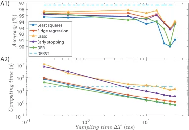
performed for several sampling times ranging from0.2ms to30ms. The accuracies for
all the methods, as a function of the sampling time, are depicted in Figure 8. Each data
point represents an average value over10different Liquids.
90 91 92 93 94 95 96 97
Least squares Ridge regression Lasso
Early stopping OFR
OFRST
10-1 100 101
10-1 100 101 102 103
A1)
[image:23.612.111.494.166.430.2]A2)
Figure 8: Comparison between the proposed OFRST method and LS, RR, lasso, ES
and OFR for different values of the sampling time∆T: accuracies (A1) and computing
times (A2).
The results show that the classification accuracy for the LS, RR, lasso, ES and
clas-sical OFR methods can be increased by decreasing the sampling time. However, the
performance is still below the one achieved by the OFRST method, which selects
presy-naptic connections using the exact spike times generated by the Liquid neurons. The
difference in accuracy between OFR and OFRST, which is expected to vanish when
Interestingly, even for∆T = 0.2ms, which is the sampling time used for simulating
the LSM, OFRST still performs significantly better than the other methods. This is
because all the training methods based on the standard Readout architecture are subject
to an approximation error when estimating the weights, for any∆T >0.
Example 3. Binary classification: selecting relevant presynaptic neurons.
This numerical example evaluates the performance of the OFRST in selecting the
relevant presynaptic partners using exact spike timing. The SNN used in this example
has a reservoir consisting of two sub-networks that are disconnected from one another,
each sub-network consisting of a different pool of 135 spiking neurons generated as
in examples 1 and 2. Two templates were generated as Poisson spike trains with
fre-quency of 20 Hz over interval [0,0.5s]. The first pool R1 = {r1, . . . , r135} receives
200 inputs generated by jittering the two spike train templates, 100 for each class, of
which 50were used for training and 50for validation. The jitter noise is drawn from
the Gaussian distribution with zero mean and standard deviation1ms. The second pool
R2 = {r136, . . . , r270}receives a number of200new jittered inputs generated from the
same two templates but in a different order selected at random.
The task is to classify the inputs to sub-networkR1 using the neuron outputs from
the full reservoir. The OFRST algorithm is compared with the LS, RR, lasso, ES and
the OFR algorithms, which use the standard filtered spike train outputs.
In essence, when solving the binary classification problem, the algorithms should
only select neurons fromR1 as pre-synaptic partners of the Readout unit. The training
Table 2.
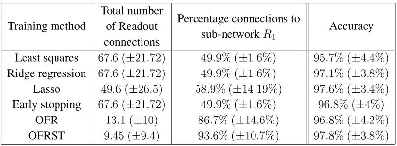
Table 2: Binary classification results for least squares, ridge regression, lasso, early
stopping, standard OFR and OFRST using two unconnected sub-networks with 135
neurons each. The reported values represent means (±standard deviations) computed
over100trials.
Training method
Total number of Readout connections
Percentage connections to sub-networkR1
Accuracy
Least squares 67.6 (±21.72) 49.9% (±1.6%) 95.7% (±4.4%)
Ridge regression 67.6 (±21.72) 49.9% (±1.6%) 97.1% (±3.8%)
Lasso 49.6 (±26.5) 58.9% (±14.19%) 97.6% (±3.4%)
Early stopping 67.6 (±21.72) 49.9% (±1.6%) 96.8% (±4%)
OFR 13.1 (±10) 86.7% (±14.6%) 96.8% (±4.2%)
OFRST 9.45 (±9.4) 93.6% (±10.7%) 97.8% (±3.8%)
The results show that OFRST achieves the highest accuracy among all methods
us-ing the least number of Readout presynaptic connections, and the highest percentage of
connections to the correct sub-networkR1.Only OFR and OFRST achieve a percentage
of connections toR1of over90%, while all the other methods result in percentages just
above chance.
Example 4. Motion direction decoding using multi-electrode array recordings
from the primary visual cortex.
Here we use the proposed methodology to decode stimulus features using
simul-taneous multi-electrode array recordings of visually evoked activity from the primary
visual cortex of three anesthetized macaque monkeys. The data were downloaded from
monkey number1.
The stimuli were full-contrast drifting sinusoidal gratings at12orientations spaced
equally (0◦,30◦,60◦, . . . ,270◦). Each stimulus was presented200times, for a duration
of1.3s per trial (Smith & Kohn, 2008; Kelly et al., 2010). The spiking train responses
of106 neurons were simultaneously recorded using a Utah multi-electrode array and
spike-sorted offline (Smith & Kohn, 2008; Kelly et al., 2010). In this example we only
use the first 200 ms from all recording trials, which is the time reported for visual
categorisation tasks in primates (Fabre-Thorpe, 1998; Hung et al., 2005). A recording
trial for the0◦ drifting bar stimulus is depicted in Figure 5.
0 0.05 0.1 0.15 0.2
0 20 40 60 80 100
[image:26.612.119.502.330.549.2](a)
(b)
Figure 9: The first sweep of experimental data used in Example 4: a) The first frame
of a drifting bar stimulus oriented at 0◦, b) Raster plot showing the response of 106
neurons, as a function of time.
The decoding task is to predict the stimulus orientation based on the recorded neural
directions was assigned a target label (1−12) and a Readout. Each Readout processes
the outputs of the106recorded neurons, which play the role of the Liquid spike train
outputs.
The data (2400 trials) was randomly divided into equal datasets for training and
validation, such that each dataset comprises100 trials with each of the12inputs. The
12Readouts were trained using the "one-to-all" method, also known as "1-hot coding",
where only one Readout generates an output "1" at any given time. Specifically, the
tar-get output for each Readout satisfiesy∗(t) = 1when the input direction label matches
the Readout label, andy∗(t) = −1 for any other direction. The overall prediction is
given by the label of the Readout with maximum average value. The training data for
each Readout consists of100trials from the target class and100trials evenly distributed
among all other classes. The parameters of the12Readouts were tuned using the LS,
RR, lasso, ES and the OFRST methods. Considering the large number of possible
con-nections, here the OFRST algorithm for each Readout was stopped when the criterion
ERRp < ζ was met, whereζ = 4·10−4 is a parameter determined using line search
andERR denotes the error reduction ratio (see Appendix 4). Essentially, this means
that each Readout only connects to presynaptic neurons whose outputs contribute more
than0.04% to the variance change in the target output. The regularization parameters
for RR and lasso, and the number of iterations for ES were selected using line search to
maximise the accuracy on the validation dataset. The final accuracy, computed on the
validation dataset, is defined as the percentage of correctly decoded input directions.
We compared the decoding performance with standard Readouts, trained with LS,
OFRST algorithm described in subsection 3.3. The results are summarised in tables 3
[image:28.612.111.505.188.303.2]and 4.
Table 3: Multi-label classification accuracies with the standard LS, RR, lasso, ES
meth-ods and the proposed OFRST method.
Training Readout accuracy (%) Final
method 1 2 3 4 5 6 7 8 9 10 11 12 accuracy
LS 86 84 83 81 82 84 85 83 84 87 80 78 58.17%
RR 88 88 85 87 84 80 84 88 84 85 85 82 61.75%
Lasso 83 83 85 87 83 82 83 90 83 86 83 81 59.5%
ES 89 85 87 87 82 82 88 87 88 86 82 83 61.33%
[image:28.612.102.512.405.522.2]OFRST 88 88 86 86 84 86 88 86 85 89 82 84 67.58%
Table 4: Number of presynaptic connections selected for each Readout with the
stan-dard LS, RR, lasso, ES methods and the proposed OFRST method.
Training Number of Readout connections
method 1 2 3 4 5 6 7 8 9 10 11 12
LS 106 106 106 106 106 106 106 105 105 106 106 106
RR 106 106 106 106 106 106 106 106 106 106 106 106
Lasso 69 71 62 77 69 70 68 64 75 77 72 72
ES 106 106 106 106 106 106 106 106 106 106 106 106
OFRST 49 61 63 61 66 59 58 61 60 60 61 59
The results show that the proposed spike time based Readout, trained with the
OFRST algorithm, performs significantly better than the standard Readout architecture
trained with LS, RR, lasso, or ES, while using significantly fewer neuron connections.
Example 5. Speech recognition.
recog-nition. The data is a subset of the TI-46 corpus of isolated spoken digits, consisting of
500utterances of digits "zero" to "nine" spoken by5different female speakers 1
(Dod-dington & George, 1981; Schalk, 1982).
The decoding task is to predict the digit number using a LSM, formulated as a
multi-label classification problem (Verstraeten et al., 2005). The LSM in this example has135
neurons, spatially organised as a lattice with dimensions 15x3x3. As before, each digit
was assigned a target label (1-10) and a Readout unit.
The data is preprocessed using the Lyon passive ear model, which is a model of
the human inner ear, or cochlea. This model consists of three processing stages: a
band-pass filter-bank, inspired by the human ear sensitivity to certain frequencies, half
way rectification, and automatic gain control, which model the hair cells in the cochlea
(Lyon , 1982). Subsequently, the continuous output of the Lyon passive ear model is
converted into a spike train using an algorithm called Ben’s spiker algorithm (BSA)
(Schrauwen, 2003). This preprocessing front-end, consisting of the Lyon passive ear
model in series with BSA, has been used successfully to address this type of speech
recognition problem using an LSM (Verstraeten et al., 2005, 2007; Yin et al., 2012).
The data was divided in two sets: a training set of size300and a validation set of size
200, such that the recordings of each speaker are proportionally distributed between the
two sets. As before, the10Readouts were trained using the "one-to-all" method. The
training data for each Readout consists of 60recordings from the corresponding target
class and 60recordings evenly distributed among all other classes. The final accuracy
1Downloaded from the Linguistic Data Consortium website:
is defined as the percentage of correctly recognised digits in the validation dataset.
The10Readout units were trained using LS, RR, lasso, ES and the OFRST method.
The stop criterion for the OFRST algorithm isERRp+1−ERRp < ζ. The parameter
ζand the regularization parameters for RR, lasso and ES were tuned for each Readout
on the validation dataset using line search.
The comparative performance of the spike time based Readouts trained with OFRST,
and the standard Readouts trained with LS, RR, lasso and ES are summarised in tables
[image:30.612.136.481.388.636.2]5 and 6.
Table 5: Multi-label classification accuracies for the LS, RR, lasso, ES methods and the
proposed OFRST method, computed as mean (± standard deviation) for 10different
Liquid simulations.
Training Readout accuracy (%)
method 1 2 3 4 5 6
LS 88(±6) 96(±3) 96(±2) 95(±4) 94(±4) 95(±4)
RR 95(±3) 92(±3) 91(±6) 93(±5) 95(±3) 93(±4)
Lasso 96(±2) 90(±2) 87(±7) 92(±7) 95(±4) 91(±4)
ES 96(±3) 92(±3) 92(±5) 94(±6) 95(±3) 93(±5)
OFRST 94(±4) 95(±3) 100(±1) 91(±4) 98(±2) 93(±7)
Training Readout accuracy (%) Final
method 7 8 9 10 accuracy
LS 97(±3) 94(±1) 92(±5) 95(±4) 73.4%(±5.5%)
RR 100(±1) 92(±4) 89(±5) 91(±2) 86.4%(±2.9%)
Lasso 99(±1) 92(±4) 83(±8) 89(±4) 85.9%(±2.2%)
ES 99(±1) 91(±4) 89(±4) 91(±3) 86.6%(±2.4%)
OFRST 99(±1) 92(±5) 99(±2) 90(±3) 88%(±1.9%)
The results show that the proposed spike based Readout architecture trained with
More-Table 6: The average number of presynaptic connections selected for each Readout
using the LS, RR, lasso, ES methods and the proposed OFRST method, computed for
10different Liquids.
Training Average number of Readout connections
method 1 2 3 4 5 6 7 8 9 10
LS 112 112 112 112 112 112 112 112 112 112
RR 112 112 112 112 112 112 112 112 112 112
Lasso 87 82 85 86 85 86 90 88 85 85
ES 112 112 112 112 112 112 112 112 112 112
OFRST 61 54 60 59 63 67 66 68 65 58
over, each spike based Readout trained with OFRST has significantly fewer connections
to Liquid neurons compared to the corresponding standard Readout trained with LS,
RR, lasso and ES. Relative to lasso, which results in the fewest presynaptic connections
for the standard Readout, the proposed OFRST method leads to a total reduction of28%
[image:31.612.132.482.159.279.2]5 Conclusions
This work proposed a spike based Readout architecture for LSMs and introduced a
new training method that uses the exact spike timing information generated by SNN
models, or recorded during experimental procedures. The new method implements an
orthogonal forward regression algorithm for training the Readout parameters, which
exploits a distance metric defined in a spike train space.
The new algorithm, called orthogonal forward regression with spike trains (OFRST),
allows the selection of the connectivity between the Liquid and the Readout unit, i.e.,
the neurons in the Liquid that are particularly relevant for solving a given learning or
decoding task.
One advantage is that computations are carried out directly on spike trains. The
standard methods filter the spike trains and then perform uniform sampling in order to
optimise the weights. It is demonstrated theoretically and shown through numerical
simulations, with synthetic and experimental data, that the classification accuracy is
improved by using exact spike times.
Specifically, new theoretical results demonstrated that the proposed Readout trained
with OFRST outperforms the standard Readout, which combines linearly the uniform
samples from the neuron filtered outputs and is trained with ordinary least squares,
ridge regression, lasso or early stopping. Numerical simulations with synthetic data
confirmed the theoretical findings and also showed that the proposed algorithm leads to
outperforms the standard methods on decoding the orientation of drifting gratings using
the multi-electrode array recordings of the evoked activity in the primary visual cortex
of the monkey. An additional example showed the advantage in using the OFRST
method on a speech recognition task.
It is interesting to highlight the fact that typically around less than20%of the total
possible connections between Liquid and Readout are required, and that fully connected
Readouts achieve less accuracy on classification tasks. This suggests that, besides
de-coding stimulus features from the evoked brain activity, the new training method could
also be used to characterise the functional specificity of neurons in the brain.
Appendix 1. Proofs of theorems
Proof of Theorem 1. The mapping (4) is well defined if the operator
F
:Sout → FSoutis well defined and invertible.
A functiony∈FSoutsatisfies
y(t) = N
X
k=1
wk
F
soutk (t) =F
NX
k=1
wksoutk
!
(t).
According to the definition of Sout it follows thatPN
k=1wksoutk ∈ Sout, and therefore
F
: Sout → FSout is well defined. Moreover,F
is invertible if it is a one-to-one andonto operator. Lets1 =PNk=1vksoutk ands2 =PNk=1wksoutk .Operator
F
is one-to-oneif
F
s1 =F
s2 ⇒s1 =s2.It follows that
F
s1 =F
s2 ⇔N
X
k=1
vk
F
soutk (t) = NX
k=1
wk
F
soutk (t)⇔ NX
k=1
The functions{
F
soutk }Nk=1 are linearly independent according to Remark 1. It
fol-lows that wk =vk,∀k = 1, . . . , N, and thus
F
is one-to-one. According to thedefini-tion of FSout and due to the linearity of
F
, it follows thatF
is also an onto operator,and thus it is invertible.
Proof of Theorem 2.
ky∗−
R
wFsoutk2L2 =ky∗−R
wF1
sout1 , . . . ,F
NsoutNk2L2
=ky∗−
N
X
n=1
wn
F
soutn k2L2=ky∗−
F
N
X
n=1
wnsoutn k2L2
=ky∗−
F
R
¯ws outk2L2
=ky∗k2
L2 +k
F
R
¯ws outk2
L2 −2
y∗,
F
R
¯ws out
L2
=ky∗k2L2 +k
F
R
¯ws outk2L2 −2
P
FSout(y∗),F
R
¯ws outL2
=ky∗k2L2 +k
F
R
¯ws outk2L2 −2
F
sy∗,F
R
¯ws outL2
=ky∗k2L2 +
1 2k
R
¯wsout
k2S−
sy∗,
R
¯ws outS
= 1
2
k
R
¯wsout
k2S+ksy∗k2S−2
sy∗,
R
¯ws outS
− 12ksy∗kS2+ky∗k2L2
= 1
2ks y∗
−
R
¯wsoutk2S−1 2ks
y∗
k2S+ky
∗
Appendix 2. The Standard Orthogonal Forward Regression Algorithm (OFR)
LetERR(jp)be the error reduction ratio corresponding to termxj at iterationpdefined
as
ERR(jp)=
D
x⊥(j p), y∗E2
L2
kx⊥(j p)k2
L2 · ky∗k2L2 .
The algorithm for training the Readout weights and predicting the input class is
given as follows.
• Initialization
– x⊥(1)j =xj, j = 1, . . . , N,
– ℓ1 = argmax
j∈{1,...,N}
ERRj(1), L(1) ={ℓ 1},
– ERR1 =ERR(1)ℓ1 ,
– x⊥
1 =xℓ1, w
⊥ 1 =
hy∗,x⊥ 1iL2 kx⊥
1k2L2
,
– w1 =w⊥1.
• Forp= 2, . . . , N, compute:
– x⊥(j p) =x⊥(j p−1)−hxj,x⊥p−1iL2 kx⊥
p−1k2L2
, j ∈ {1, . . . , N}\L(p−1),
– ℓp = argmax j∈{1,...,N}\L(p−1)
ERR(jp), L(p) =L(p−1)∪ {ℓ
p},
– ERRp =ERR(ℓpp),
– x⊥
p =xℓp, w ⊥
p =
hy∗,x⊥
piL2 kx⊥
pk2L2 ,
– ai,p =
hxi,x⊥piL2 kx⊥
– A(p) =
1 a1,2 . . . a1,p
0 1 . . . a2,p
. . . .
0 0 . . . ap−1,p
0 0 . . . 1
,
– w⊥(p)= [w⊥
1, . . . , wp⊥],
– w(p)=A(p)−1w⊥(p)
,
wherew(p) = [w(p)
1 , . . . , w (p)
p ]denote the Readout weights at iterationp,
– yˆ(p)=Pp
k=1w (p)
k xℓp,
whereyˆ(p)is the Readout output,
– P red yˆ(p)
=signhRTmax
0 yˆ(p)(t)dt
i
,
whereP red yˆ(p)
is the class prediction based on the Readout activity on
time interval[0, Tmax], and sign()denotes the sign function.
• Select the smallestpthat gives the minimum error for validation.
Appendix 3. The Orthogonal Forward Regression with Spike Trains Algorithm
(OFRST)
LetERR(jp) be the error reduction ratio corresponding to presynaptic neuronj at
itera-tionpdefined as
ERRj(p) =
D
s⊥(j p), sy∗E2
S
ks⊥(j p)k2
S· ksy∗k2S
.
The target output spike trainsy∗is unknown prior to training. However, fory∗(t) =
±1, the inner producths, sy∗i
time interval[T1, T2], representing the total simulation time, as follows
hs, sy∗iS= 2h
F
s,F
s y∗iL2
= 2h
F
s, y∗iL2
= (±1)τs M
X
k=1
ak
h
e−max{T1τs,tk}−tk −e−
max{T2,tk}−tk τs
i
.
The algorithm for training the Readout weights and predicting the input class is
given as follows.
• Initialization
– s⊥(1)j =sout
j , j = 1, . . . , N,
– ℓ1 = argmax
j∈{1,...,N}
ERRj(1), L(1) ={ℓ 1},
– ERR1 =ERR(1)ℓ1 ,
– s⊥
1 =soutℓ1 , w
⊥ 1 =
hsy∗,s⊥ 1iS
ks⊥ 1k2S ,
– w1 =w⊥1.
• Forp= 2, . . . , N, compute:
– s⊥(j p)=s⊥(j p−1)− hsoutj ,s⊥p−1iS
ks⊥
p−1k2S
, j ∈ {1, . . . , N}\L(p−1),
– ℓp = argmax j∈{1,...,N}\L(p−1)
ERR(jp), L(p) =L(p−1)∪ {ℓ
p},
– ERRp =ERR(ℓpp),
– s⊥
p =soutℓp , w ⊥
p =
hsy∗,s⊥
piS
ks⊥
pk2S ,
– ai,p =
hsout i ,s⊥piS
ks⊥
– A(p) =
1 a1,2 . . . a1,p
0 1 . . . a2,p
. . . .
0 0 . . . ap−1,p
0 0 . . . 1
,
– w⊥(p)= [w⊥
1, . . . , wp⊥],
– w(p)=A(p)−1w⊥(p)
,
wherew(p) = [w(p)
1 , . . . , w (p)
p ]denote the Readout weights at iterationp,
– sˆ(p)=Pp
k=1w (p)
k soutℓp ,
wheresˆ(p)is the Readout output,
– P red ˆs(p)
=sign "
Tmax−2τsPMk=1p a (p)
k e
−Tmax−t
(p)
k
τs −1
!#
,
where P red sˆ(p)
is the class prediction based on the Readout activity
on time interval [0, Tmax], sign() denotes the sign function, and sˆ(p) =
n
a(kp), t(kp)oMp
k=1.
• Select the smallestpthat gives the minimum error for validation.
Acknowledgments
DF and DC gratefully acknowledge that this work was supported by BBSRC under
grant BB/M025527/1. We also gratefully acknowledge reviewers’ comments, which
References
Bishop, C. M. (2006). Pattern recognition and machine learning.Springer.
Billings, S. A., Chen, S., & Korenberg, M. J. (1989). Identification of MIMO non-linear
systems using a forward-regression orthogonal estimator. International journal of
control,46(6), 2157–2189.
Bohte, S., Kok J. & Poutre H. L. (2002). Errorbackpropagation in temporally encoded
networks of spiking neurons. Neurocomp,48(1-4), 17–37.
Carnell, A., & Richardson, D. (2005). Linear algebra for time series of spikes. InProc.
European Symp. on Artificial Neural Networks.
Chen, S., Billings, S. A., & Luo, W. (1989). Orthogonal least squares methods and their
application to non-linear system identification. International Journal of Control,50
(5), 1873 – 1896.
Doddington, G. R. & Schalk, T. B. (1981). Speech recognition: turning theory to
practice. IEEE Spectrum, 26 – 32.
Dolinský, J., Hirose, K., & Konishi, S. (2017). Readouts for echo-state networks built
using locally-regularized orthogonal forward regression. Journal of Applied
Statis-tics,45(4), 740–762.
Fabre-Thorpe, M., Richard, G., & Thorpe, S. J. (1998). Rapid categorization of natural
Florescu, D. (2017). Reconstruction, identification and implementation methods for
spiking neural circuits.Springer.
Florescu, D., & Coca, D. (2018). Identification of Linear and Nonlinear Sensory
Pro-cessing Circuits from Spiking Neuron Data. Neural Computation,30(3), 670–707.
Florescu, D., & Coca, D. (2015). A novel reconstruction framework for time-encoded
signals with integrate-and-fire neurons. Neural Computation,27(9), 1872–1898.
Florian, V. (2007). Reinforcement learning through modulation of
spike-timing-dependent synaptic plasticity. Neural Computation,19(6), 1468–1502.
Florian, V. (2012). The Chronotron : A Neuron That Learns to Fire Temporally Precise
Spike Patterns. PloS one,7(8).
Gardner, B., & Grüning, A. (2016). Supervised learning in spiking neural networks for
precise temporal encoding. PloS one,11(8).
Gollisch, T., & Meister, M. (2008). Rapid neural coding in the retina with relative spike
latencies. Science,319(5866), 1108–1111.
Gütig, R. (2014). To spike, or when to spike? Current opinion in neurobiology, 25,
134–139.
Häusler, S., & Maass, W. (2007). A statistical analysis of information-processing
prop-erties of lamina-specific cortical microcircuit models. Cerebral cortex, 17(1), 149–
162.
dynamics of neural microcircuits from the point of view of low dimensional readouts.
Neural Comput,14(11), 2531–2560.
Hirata, Y., Katori, Y., Shimokawa, H., Suzuki, H., Blenkinsop, T. A., Lang, E. J., &
Aihara, K. (2008). Testing a neural coding hypothesis using surrogate data. Journal
of neuroscience methods,172(2), 312–322.
Houweling, A. R., & Brecht, M. (2008). Behavioural report of single neuron stimulation
in somatosensory cortex. Nature,45165–68.
Huber, D., Petreanu, L., Ghitani, N., Ranade, S., Hromádka, T., Mainen, Z., & Svoboda,
K. (2008). Sparse optical microstimulation in barrel cortex drives learned behaviour
in freely moving mice. Nature,451, 61–64.
Hung, C. P., Kreiman, G., Poggio, T., & DiCarlo, J. J. (2005). Fast readout of object
identity from macaque inferior temporal cortex. Science,451(5749), 863–866.
Izhikevich, E. M. (2006). Polychronization: Computation with Spikes.Neural Comput,
18(2).
Izhikevich, E. M. (2007). Solving the distal reward problem through linkage of STDP
and dopamine signaling. Cerebral cortex,17(10), 2443–2452.
Jaeger, H.(2001). The echo state approach to analysing and training recurrent neural
networks. Technical Report GMD Report 148, German National Research Center for
Information Technology, 2001.
Jones, L. M., Depireux, D. A., Simons, D. J., & Keller, A. (2004). Robust temporal
Kayser, C., Montemurro, M. A., Logothetis, N. K., & Panzeri, S. (2009). Spike-phase
coding boosts and stabilizes information carried by spatial and temporal spike
pat-terns. Neuron,61(4), 597–608.
Kelly, R. C., Smith, M. A., Kass, R. E., & Lee, T. S. (2010). Local field potentials
indicate network state and account for neuronal response variability. Journal of
com-putational neuroscience,29(3), 567–579.
Kohn, A. & Smith, M. A. (2016). Utah array extracellular recordings of spontaneous
and visually evoked activity from anasthetized macaque primary visual cortex (V1).
CRCNS.org, Retrieved from: http://dx.doi.org/10.6080/KONC5Z4X.
Lukosevicius, M., & Jaeger, H. (2009). Reservoir Computing Approaches to Recurrent
Neural Network Training. Computer Science Review,3(3), 127–149.
Lazar, A. A., & Pnevmatikakis, E. A. (2008). Faithful Representation of Stimuli with a
Population of Integrate-and-Fire Neurons.Neural Computation,20(11), 2715–2744.
Lazar, A. A., & Slutskiy, Y. B. (2015). Spiking neural circuits with dendritic stimulus
processors. Journal of Computational Neuroscience,38(1): 1–24, 2015.
Lyon, R. (1982). A computational model of filtering, detection, and compression in the
cochlea. In Acoustics, Speech, and Signal Processing, IEEE International
Confer-ence on, ICASSP’82,7.
Maass, W., Natschläger, T., & Markram, H. (2002). Real-time computing without stable
states: a new framework for neural computation based on perturbations. Neural
McCulloch, W. S., & Pitts, W. (1943). A logical calculus of the ideas immanent in
nervous activity. The bulletin of mathematical biophysics.,5(4), 115–133.
Mainen, Z. F., & Sejnowski, T. J. (1995). Reliability of spike timing in neocortical
neurons. Science,268(5216), 1503–1506.
Markram, H., Wang, Y., & Tsodyks, M.(1998). Differential signaling via the same axon
of neucortical pyramidal neurons. InProc. Natl. Acad. Sci., 95, 5323–5328.
Memmesheimer, R. M., Rubin, R., Ölveczky, B. P., & Sompolinsky, H. (2014).
Learn-ing precisely timed spikes. InNeuron, 82(4), 925–938.
Natschläger, T., Markram, H., & Maass, W. (2003). Computer models and analysis
tools for neural microcircuits. InNeuroscience Databases. Springer, Boston, MA.
Nicola, W., & Clopath, C. (2017). Supervised learning in spiking neural networks with
FORCE training. InNature communications, 8(1).
Pfister, J. P., Toyoizumi, T., Barber, D., & Gerstner, W. (2006). Optimal
spike-timing-dependent plasticity for precise action potential firing in supervised learning. Neural
Comput,18(6), 1318–1348.
Ponulak, F., & Kasinski, A. (2010). Supervised learning in spiking neural networks
with ReSuMe: sequence learning, classification, and spike shifting. Neural Comput,
22(2), 467–510.
Riehle, A., Grün, S., Diesmann, M., & Aertsen, A. (1997). Spike synchronization
and rate modulation differentially involved in motor cortical function. Science, 278
Seth, A. K. (2015). Neural coding: rate and time codes work together.Current Biology,
25(3), 357–363.
Schalk, T. B.(1982). The Design and Use of Speech Recognition Data Bases.
Proceed-ings of the Workshop on Standardization for Speech I/O Technology, 25 (3), 211 –
214.
Schrauwen, B., & Van Campenhout, J. (2003). BSA, a fast and accurate spike train
encoding scheme. In Proceedings of the international joint conference on neural
networks,4(4), Piscataway, NJ: IEEE.
Smith, M. A.,z & Kohn, A. (2008). Spatial and temporal scales of neuronal correlation
in primary visual cortex. Journal of Neuroscience,28(48), 12591–12603.
Srivastava, K. H., Holmes, C. M., Vellema, M., Pack, A. R., Elemans, C. P.,
Nemen-man, I., & Sober, S. J. (2017). Motor control by precisely timed spike patterns. In
Proceedings of the National Academy of Sciences,114(5), 1171-1176.
Thomson, A. M., West, D. C., Wang, Y., & Bannister, A. P. (2002). Synaptic
connec-tions and small circuits involving excitatory and inhibitory neurons in layers 2-5 of
adult rat and cat neocortex: triple intracellular recordings and biocytin labelling in
vitro. Cerebral cortex,12(9), 936–953.
Verstraeten, D., Schrauwen, B., D’Haene, M., & Stroobandt, D. (2007). An
experimen-tal unification of reservoir computing methods. Neural networks,20(3), 391-403.
word recognition with the liquid state machine: a case study. Information Processing
Letters,95(6), 521-528.
Vigneswaran, G., Philipp, R., Lemon, R. N., & Kraskov, A. (2013). M1 corticospinal
mirror neurons and their role in movement suppression during action observation.
Curr Biol,23(3).
Wolfe, J., Houweling, A. R., & Brecht, M. (2010). Sparse and powerful cortical spikes.
Current opinion in neurobiology.,20(3), 306–312.
Xu, Y., Zeng, X., Han, L., & Yang, J. (2013). A supervised multi-spike learning
algo-rithm based on gradient descent for spiking neural networks. Neural Networks, 43,
99–113.
Yin, J., Meng, Y., & Jin, Y. (2012). A developmental approach to structural
self-organization in reservoir computing. IEEE transactions on autonomous mental