Computational flow analysis of a dual chamber vortex generator for an absorption refrigeration system

Rochester Institute of Technology

RIT Scholar Works

Theses

Thesis/Dissertation Collections

2-1-2001

Computational flow analysis of a dual chamber

vortex generator for an absorption refrigeration

system

Amilcar Ramos

Follow this and additional works at:

http://scholarworks.rit.edu/theses

This Thesis is brought to you for free and open access by the Thesis/Dissertation Collections at RIT Scholar Works. It has been accepted for inclusion

in Theses by an authorized administrator of RIT Scholar Works. For more information, please contact

[email protected]

.

Recommended Citation

Computational Flow Analysis of a Dual Chamber Vortex

Generator for an Absorption Refrigeration System

By

AmI1car R. Arvelo Ramos

A Thesis Submitted in Partial Fulfillment of the Requirement for the Degree of

.Master of Science in Mechanical Engineering

Approved by:

Dr. Ali Ogut

Department of Mechanical Engineering.

Dr. Amitabha Ghosh

Department of Mechanical Engineering.

Dr. P. Venkataraman

Department of Mechanical Engineering.

Dr. Edward Hensel

Department Head of Mechanical Engineering.

Thesis Advisor

Department of Mechanical Engineering

College of Engineering

Rochester Institute of Technology

Rochester, New York 14623

PERMISSION TO REPRODUCE THE THESIS

Title of Thesis

Computational Flow Analysis of a Dual Chamber

Vortex Generator for an Absorption Refrigeration System

I, Anu1car

R.

Arvelo Ramos, hereby grant permission to the Wallace Memorial Library of

Rochester Institute of Technology to reproduce my thesis in whole or in part.

Any

reproduction will not be for commercial use of profit.

DEDICATION

I

would

like

to

dedicate

thisworkto

my

parents,

Rafael Arvelo Medina

and

Aida Luz Ramos

Arce,

for

alltheir

love

andunderstanding.

For

theeducation

they

gave_me, and

for giving

me

support and

helping

me

in

all

my dreams

to cometrue.

Thank

you

for

always

being

present

besides

throughalltheunforgettableyears andencourage meto strive upwards.

Also,

I

would

like

to

dedicate

thiswork to

my devoted

wife

Rebecca Ortiz for her

assistance,

ACKNOWLEDGMENTS

I

would

like

to thank thosepeople who provided assistance and supporttomeoverthecourse

ofthis project.

First

and

foremost,

I

would

like

to thank

my

parents

for giving

methe moral

supporttomake allthispossible.

I

would

like

to thank

my

cousin

Gloribel Arvelo

and

her husband Robert Park for

their

availability in

helping

me while

I

was

doing

my Master

of

Science

in

Mechanical

Engineering.

I

would

like

to thank

my

thesis advisor,

Dr. Ali

Ogut,

for his

guidance and support ofthis

thesis.

A

special thanks to

God,

for giving

me the strength tonever give

up

and make possible

my

ABSTRACT

A

significant amount of

low

temperature

(between

60C

and

99C)

heat is

wasted

annually in

industrial

processes.

This

wasted

heat has

the potential to

drive

absorption regrigeration

systems with the

penalty

of

lowering

the

COP (Coefficient

of

Performance)

oftheabsorption

regrigeration system.

An

absorption refrigeration system with avortexgenerator, permitsthe

useof

low

temperature waste

heat

as an

energy

source with

improved

generator

capacity

and

COP.

The

vortex generator

is

a

device

that consists of two chambers

(lower

and upper

chamber) and

is

usedtoseparatetherefrigerant

from

theabsorbent

in

absorption refrigeration

system

by

a cavitationprocesscaused

by

the

strong swirling flow

withinthechamber.

The

scope ofthis project

is

to predict,

by

CFD

analysis, thepressure

drop

toward the center

ofthechamber, andobserve

how

the

free

surface area generated

by

the

strong

swirling flow

is influenced

by

the

inlet velocity

and vortex chamber configuration.

Also,

based

on the

results ofthe

investigation,

determine

theoptimized

design.

It

can

be

concluded thatthe

free

surface area generated

by

the

swirling flow increases

when

the

inlet velocity increases

and when the vortex chamber aspect ratio

(diameter/height, D/H)

decreases.

Also,

by

placing

the

inlet

ofthe vortex chamber at the mid-height ofthe vortex

chamber will

increase

the size of the

free

surface area.

The

free

surface area can

be

optimized when the vortex chamber

dimensions

are

D

=

16.12

_cm

,

H

=

16.12

cm

(aspect

ratio=

1),

with

inlet

placed atthemid-heightofthechamber.

For

optimum _{results, the}

inlet

TABLE

OF

CONTENTS

LIST

OF FIGURES

ix

LIST OF

TABLES

xii

LIST

OF

SYMBOLS

xiii

CHAPTER

ONE. INTRODUCTION

1

1.1

Project

Background

1

1.2

Project

Objectives

and

Goals

2

1

.3

Description

ofthe

Dual

Vortex Chamber Generator

4

1

.4

Absorption

Refrigeration

Cycle

6

1.5

Vortex

Flow

Theory

9

CHAPTER TWO. FLUID FLOW

THEORY

16

2.1

The

Mass Conservation Equation

16

2.2

The Momentum Equations

18

2.3

Turbulent

Flow

22

2.4

Free Surface

Theory

24

CHAPTER THREE. Computational Fluid

Dynamics

Analysis

28

3.1

CFD Code

Introduction

28

3.2

Model Generation

30

3.3

Initial Conditions

30

3.4

Mode

Meshing

and

Boundary

Conditions

33

3.4.1

Meshing

33

3.5

Model

Study

35

3.6

Model

Parameters

37

3.7

Cases Studied

39

3.8

Vortex Reynolds Number

40

3.9

Pressure

Drop

42

3.9.1

Inlet

42

3.9.2

Bottom Outlet

45

3.10

Calculation

of

Free

Surface

Area

46

CHAPTER FOUR.

Results

and

Discussion

48

4. 1

Introduction

48

4.2

Model Mesh

49

4.3

Initial Conditions

52

4.3.1

Initial Fluid Distribution

52

4.3.2

Initial Pressure Distribution

54

4.3.3

Initial

Velocity

Vectors Distribution

57

4.4

Steady

State Solution

58

4.5

Results

of

Cases Studied

61

4.5.1

Comparison

of

Different Void Pressures

64

4.5.2

Comparison

of

Mass Flow

Rates

65

4.5.3

Comparison

of

Surface Area

vs.

Inlet

Velocity

66

4.6

Vortex Chamber Pressure Distribution

67

4.6.1

Pressure Distribution

in

the

Vortex Chamber

67

4.6.3

Pressure

Drop

atthe

Inlet

ofthe

Vortex Chamber

72

4.6.4

Pressure

Drop

atthe

Bottom Outlet

ofthe

Vortex Chamber

73

4.7

Pressure Contour

and

Velocity

Vector Plots

74

4.7. 1

Side View

of

Pressure

and

Velocity

Vector Plots

74

4.7.2

Top

View

of

Pressure

and

Velocity

Vector Plots

79

4.8

Optimized Vortex Chamber Design

85

4.8. 1

Pressure Distribution for

the

Optimized Design

86

4.8.2

Velocity

Magnitude

and

Vectors

for

the

Optimized Design

92

4.8.3

Pressure

and

Velocity

Equations

for

the

Optimized Vortex Chamber

98

CHAPTER FIVE.

Conclusions

105

CHAPTER SIX. Recommendations

108

REFERENCES

1 1 1

APPENDIXES

114

Appendix A. Example

of

Calculation

for Pressure

Drop

at

Vortex

Chamber Inlet

115

Appendix B. Example

of

Calculation for Pressure

Drop

at

Vortex

Chamber Outlet

118

Appendix C. Example Calculation

of

Vortex Chamber Surface Area

120

Appendix D. Procedure for Development

of

Pressure

and

Velocities Equation for

the

Optimized Vortex Chamber

122

Appendix E. Equilibrium

chart

for

aqueous

lithium

bromide

solutions

1 26

Appendix F. Specific

Gravity

of

Aqueous Solutions

of

Lithium

Bromide

127

Appendix G. Viscosities

of

Aqueous Solutions

of

Lithium Bromide

128

Appendix H. Specific Heat

of

Aqueous Lithium Bromide Solutions

129

Appendix J. The

Moody

Diagram

for

Friction Factor

131

Appendix K. Example

of

Flow 3D Input File

132

Appendix L. Data

used

for Development

of

Pressure

and

Velocity

Equations

135

LIST

OF FIGURES

Figure 1.1.

Availability

ofwaste

heat for

a range oftemperatures.

2

Figure 1.2. Free

surface area generated

by

the

high

tangential

inlet

velocity.

3

Figure 1.3. Schematic

ofthe

Vortex Chamber Generator.

5

Figure

1.4. Typical Absorption Refrigeration System.

7

Figure 1.5. Flow in

a curvedpath.

10

Figure

1.6. Force

vortex

flow.

1 1

Figure 1.7. Free

vortex

flow.

12

Figure

1.8. Pressure

and

velocity distribution in

atypicalvortex

flow

application.

14

Figure 2.1

Differentialelement

for

mass

balance.

16

Figure 2.2. Stresses acting

onarectangular

fluid

particle.

19

Figure

2.3

Partially

filled

cell.

26

Figure

3.1.

Vortex Chamber

schematicwith

boundary

conditions symbols.

34

Figure 3.2. Lower Chamber Schematic

with

boundary

conditions.

35

Figure

3.3.

Detail

of

inlet

pipeand

fittings.

42

Figure 3.4. Detail

of modified

inlet.

43

Figure

3.5.

Detail

of

bottom

outlet pipe.

45

Figure 4.1

Mesh

example

in

thex-z plane

for

theoptimizedchamber

design.

49

Figure 4.2

Mesh

example

in

they-z plane

for

theoptimizedchamber

design.

5 1

Figure 4.3 Mesh

example

in

the

x-y

plane

for

theoptimized chamber

design.

52

Figure 4.4 Initial fluid

contour plot

in

x-z plane.

53

Figure 4.5

Initial fluid

contour plot

in x-y

plane.

54

Figure 4.6

Initial

pressure

distribution

contour plot

in

x-zplane.

55

Figure

4.7 Initial

pressure

distribution

contour plot

in x-y

plane.

56

Figure 4.8 Initial velocity

distribution

contour plot

in x-y

plane.

57

Figure 4.9 Volume

of solution

in

thevortex chamberwithtime.

59

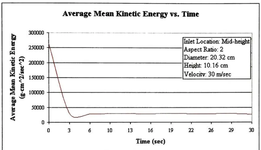
Figure

4.10 Average

mean

kinetic

energy

withtime.

60

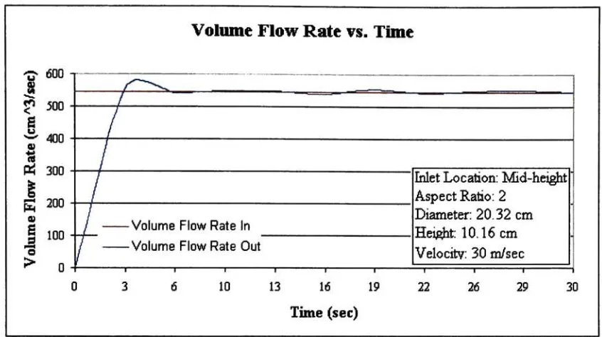
Figure

4.11

Volume flow

ratewithtime.

61

Figure 4.12 Relation

of

Surface Area

vs.

Inlet

Velocity

with

inlet

atthecenter

ofthevortex chamber.

66

Figure

4.13

Pressure distribution in

thex-zplane.

68

Figure

4.14

Pressure distribution in

theaxial

direction,

inlet

atthecenter ofthechamber.

69

Figure

4.15

Pressure distribution in

theaxial

direction,

inlet

atthe

top

ofthechamber.

70

Figure

4.16 Pressure distribution along

thex axis

for different inlet

velocities.

70

Figure

4.17 Pressure distribution in

theaxial

direction,

for different inlet

velocities.

71

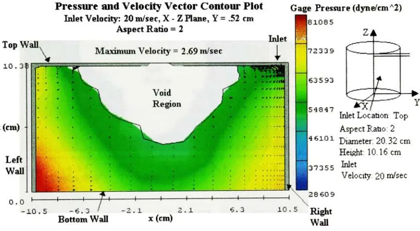
Figure 4.18

Contour Plot in

thex-zplane,

AR

=

2,

Inlet:

Top,Velocity

=

30

_m/s.

75

Figure

4.19

Contour Plot in

thex-zplane,

AR

=

2,

Inlet:

Top,Velocity

=

20

_m/s.

76

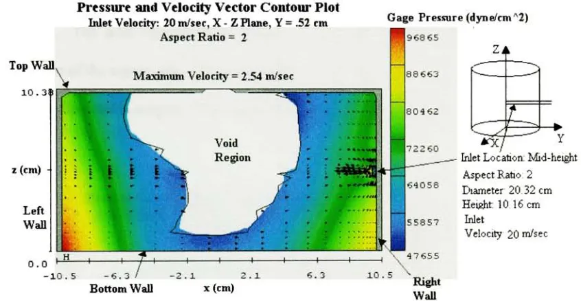
Figure 4.20

Contour Plot in

thex-z_plane,

AR=2,

Inlet:Center,

Velocity

=

20

_m/s.

77

Figure

4.21

Contour Plot

in

thex-zplane,

AR=1

.5,

Inlet:Center,

Velocity

=

20

m/s.

78

Figure 4.23

Contour Plot in

the

x-y

plane,

inlet location

at center ofthevortex chamber.

82

Figure

4.24

Contour

Plot in

the

x-y

_plane,

top

ofthevortex chamber.

83

Figure 4.25 Contour

Plot in

the

x-y

plane,

detail

ofthe

inlet

section.

84

Figure

4.26

Pressure Contour Plot

for

theoptimized

design in

the

x-y

plane at

the

bottom location

ofthevortex chamber

86

Figure 4.27 Pressure Contour Plot for

theoptimized

design in

the

x-y

planeat

themid-height elevationofthevortex chamber

88

Figure 4.28 Pressure Contour Plot for

theoptimized

design in

the

x-y

plane at

the

top

location

ofthevortex chamber

89

Figure 4.29 Pressure Contour Plot for

theoptimized

design in

the

x-y

plane

90

Figure

4.30

Velocity

Magnitude

and

Vectors

plot at

bottom

oftheoptimized chamber

93

Figure

4.31

Velocity

Magnitude

and

Vectors

plot oftheoptimized chamber

at an elevation of

3.54

cm

94

Figure 4.32 Detail

ofthe tangential

veolcity

closeto thewall

95

Figure

4.33

Velocity

Magnitude

and

Vectors

plot at a mid-height elevation

96

Figure 4.34 Graph

of

Pressure

versus

Position for

theoptimized vortexchamber

99

Figure 4.35 Graph

of

Tangential

Velocity

vs.Position fortheoptimized vortex chamber

101

Figure 4.36

Graph

of

Tangential

Velocity

vs.Position

for

theoptimized vortex chamber

for

the

boundary

layer

region

102

Figure

4.37

Graph

of

Axial

Velocity

versus

Position

for

theoptimized vortex chamber

104

Figure

G.l

Viscosities

of

Aqueous Solutions

of

Lithium Bromide

128

Figure H.l

Specific Heat

of

Aqueous

Lithium Bromide Solutions

1

29

Figure 1.1

Enthalpy

Diagram

for

Aqueous

Lithium Bromide Solutions

130

Figure J.l The

Moody

Diagram

for Friction Factor

1 3

1

LIST

OF TABLES

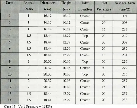
Table

3.1.

List

of

Cases

studied.

40

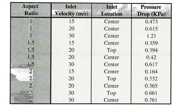
Table

4.1. Results

ofthecases studied.

62

Table 4.2. Comparison

oftheresults

for different

void pressures.

64

Table

4.3. Comparison

oftheresults

for different

mass

flow

ratesand velocities.

65

Table 4.4. Comparison

of

Free Surface Area

vs.

Inlet

Velocity

withthe

inlet

atthe

centerofthevortex chamber.

67

Table 4.5. Pressure

drop

atthe

inlet

ofthevortex chamber

for different

aspect ratios and

velocities.

72

Table

4.6. Pressure

drop

acrossthe

bottom

outlet

for

thecasesstudied.

73

Table

4.7.

Table

of power

for

eachmonomial termandcoefficients

for

thepressure equation

oftheoptimized vortex chamber

98

Table 4.8. Table

ofpower

for

each monomialtermandcoefficients

for

the tangential

velocity

equation oftheoptimized vortex chamber

1 00

Table

4.9.

Table

ofpower

for

eachmonomial termandcoefficients

for

theaxial

velocity

LIST

OF SYMBOLS

A

Cross

sectional _area,area

Ax,

Ay,

Az

Area

ofthe

fractional

open area

in

each

direction

AR

Aspect Ratio

D

Diameter

F

Fraction

of

fluid

-F

Force

vector

f

Friction

factor

FB

Body

force

Fc

Centrifugal

force

Fs

Surface force

g

Gravity

H

Vortex Chamber height

K

Turbulent kinetic energy

Kc

Contraction

coefficient

Nozzle

coefficient

L

Pipe length

M

Mass

m

Mass flow

rate

P

Pressure

q

Mean

component of

flow

variable

R,

r

Radius

Re

Reynolds

number

S

Modulus

of mean rateofstraintensor

t

Time

t

Solution

temperature

t'

Refrigerant

temperature

u, v,w

Velocity

component

in

a

Cartesian

system

V

Linear velocity

VF

Fractional

volume opento

flow (open

volume/volumeof_cell)

Vg

Tangential velocity

X

Mass

fraction

x,

y

, z

Cartesian

coordinates

Greek Letters

GC/t

Inverse Prandlt

number

for

turbulent

kinetic energy

as

Inverse Prandlt

number

for

turbulent

kinetic energy dissipation

rate

e

Turbulent kinetic energy dissipation

rate

T

Circulation

p

Density

co

Angular velocity

ju

Absolute

Viscosity

a

Axial

stress

CHAPTER

ONE

INTRODUCTION

1.1

PROJECT BACKGROUND

Waste heat

from industrial

processes and power plants

is widely

accepted as a practical

energy

source

for

absorption

heat

pumps

(Dorgan,

1995).

Heat

sources

from approximately

99C

and above

have

proven to

be

practical.

However,

a significant amount of thermal

resources

in

the range of

211

-

528

trillion

kJ (200

_and trillion

500

BTU's)

per year

in

the

form

of

low

temperature

(between

60

and

99C)

is known

to

be

wasted

(Fineblum,

1996).

Figure

1.1

below

shows the amount of

energy

source available

for

a wide range of

temperatures.

Figure 1.1

shows that

60%

of the

heat energy in

the temperature range of

interest

is

available

in hot liquids

rather than

in

gas.

This

is

an advantage

because

liquid

sources require smaller and

less

expensive

heat

exchangers.

Conventional

absorption

refrigeration systems can use a

heat

source with

lower

temperature

(temperatures below

99

C)

in

the generator

but

with the

penalty

of

lowering

both

the

COP (Coefficient Of

Availability

of

Waste Heat

600n

. 500

*S

300

200

T 100 H

0

yff.v^";MWi

1

Gaseous

I Liquid

50-59 60-99 100-120 121-148

Temperature

ofWaste Heat

(C)

149-203

Figure 1.1.

Availability

of

Waste Heat

for

a range oftemperatures

An

absorption refrigeration system

(shown

in

Figure

1.4)

that

incorporates

the

dual

vortex

chamber generator

(shown

in

Figure

1.3)

permitsgenerators

to

operate

efficiently

with

lower

temperature waste

heat

as an

energy

source with

improved

capacity

and

COP.

For

a

description

of atypical absorptionrefrigeration systemand a

dual

vortex chamber

generator,

refertosection

1.4

and

1.3

respectively.

1.2

PROJECT

OBJECTIVES AND

GOALS

The

purpose ofthis

investigation

is

to

determine

how

thevapor-liquid

interface

areagenerated

by

the

strong

swirling

flow is influenced

by

the

LiBr

-

Water

refrigerant

rich

solution

inlet

10%

by

mass of the refrigerant-rich solution

entering

the vortex chamber

in

vapor phase.

Due

to

limitations

in

the

Computational

Fluid

Dynamics

software _use,

FLOW-3D,

the

amount of vapor generated can not

be

quantified.

The

amount of vapor generated and

transferred to the vapor region

is

influenced

by

the vapor-liquid

interface

area generated

by

the

swirling

flow (refer

to

Figure

1.2).

Mass

transfer

is

a

function

of area.

This

means that

thegreaterthe surface area generated

by

the

swirling

flow,

higher is going

to

be

the amount

of vapor generated and transferred to the vapor region.

Also

it is intended

to predict the

velocity

and pressure

distribution

ofthesolution

in

thevortex chamber.

Free Surface

areagenerated

by

the_swirling

flow.

LiBr-Water

Solution

Tangential Inlet

The

size of

the

surface area

is influenced

by

theInlet

Velocity.

Figure 1.2 Free Surface

area generated

by

the

high

tangential

inlet

velocity.

To

prove

this,

FLOW-3D,

Computational

Fluid Dynamics

(CFD)

software was used.

Different

cases ofthe

lower

chamber vortex generator with

different

configurations

(aspect

ratios and

inlet

locations)

and

inlet

velocities were studied.

Simulations

were run

by

changing

one oftheparameters and

keeping

therest oftheparameters constant with purpose

The

work

involves

determining

conditions

for

separation of the refrigerant vapor

from

the

refrigerant-rich solution.

Also,

verify

the pressure gradient at the

lower

chamber.

From

the

results ofthe

investigation,

it

is hoped

that there will

be

enough

data

to

determine how

the

replacement of a conventional generator

by

a

dual

chamber vortex generator

may

affect the

efficiency

oftheprocess and whatwill

be

the

limiting

factors.

1.3

DESCRIPTION

OF THE DUAL VORTEX CHAMBER

GENERATOR

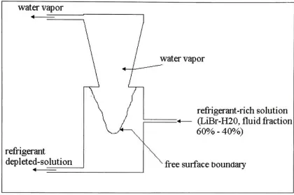
The

schematic ofthe vortex generator

is

shown

in Figure 1.3. The

vortex generator consists

oftwo chambers,

lower

chamber andupperchamber.

The

lower

chamber

is

a cylinderwith a

tangential

inlet,

atangential outlet atthe

bottom

ofthechamber anda central outlet atthe

top

ofthechamberthatconnects with theupperchamber.

The

upperchamber

has

a central

inlet

atthe

bottom

partand atangential outlet atthe

top

part.

The heated

refrigerant rich solution

(LiBr-

H20,

fluid fraction

60%

-

40%

by

weight of _solution) enters the

lower

chamber

tangentially

at conditions close to the saturation pressure.

Due

to conservation of rotational

momentum, thepressure

is

reduced towardthe central portion ofthe

lower

chamber.

Close

to the

free

surface

boundary,

the pressure will

drop

below

the saturation pressure of the

LiBr-water

solution.

This

will cause cavitation and as a result, the

heated

refrigerant-rich

water vapor

*

refrigerant

depleted-solution

water vapor

refrigerant-rich solution

:<

(LiBr-H20,

fluid

fraction

60%

-40%)

[image:20.503.42.462.63.342.2]

free

surface

boundary

Figure 1.3. Schematic

ofthe

Vortex Chamber

generator.

The

refrigerant vapor will

flow

out ofthe

swirling

mixture toward the center and upward.

The

vapor will then

flow

through the central outlet and out of the

lower

chamber

into

the

upper chamber.

The

upper chamber

is designed

as a

diffuser

with

gradually

increasing

cross-sectional area.

There,

the

swirling

vapor

is

tangentially

decelerated

as a result of

rotational momentum and the vapor pressure will

increase

prior to

leaving

through the

tangentialoutlet.

The deceleration

of

flow

in

theupper chamber

is essentially

similartowhat

occurs

in

the

diffuser

ofa compressor

(Fineblum,

1996). The

refrigerant-depleted solution

in

It

is intended

toreplacetheconventional generator

in

the

Absorption Refrigeration Cycles

by

the

Vortex Chamber

generator.

The

goal ofthe

Vortex Chamber is

to obtain

10%

by

weight

ofthe

incoming

solution

in

refrigerant vapor.

The

vortex chamber utilize the

energy

ofthe

incoming

LiBr-water

solutiontoconvert some oftherefrigerant

into

water vapor.

Therefore,

it

will required

less energy

from

an external source to generate the same amount of vapor

than

in

conventional generators.

1.4

ABSORPTION REFRIGERATION

CYCLE

In

the typical

Lithium Bromide

-Water

absorption refrigeration_cycle, asshown

in figure 1

.4,

therefrigerant

is

the waterand the absorbent

is Lithium Bromide.

The

machine consists of

four

components that exchange

energy

with surroundings, one

internal heat

exchanger, two

flow

restrictors, and a pump.

The

four

components that exchange

energy

with the

surroundings are _{the condenser, generator,} evaporator and absorber.

The

machine operates

between

two

working

pressures, the

high

pressureside

(typically

6

KPa)

andthe

low

pressure

side

(typically

1 KPa).

The high-pressure

side

is

at the generator and _condenser, and the

low-pressure

side

is

attheabsorber andevaporator.

The

pressure

is determined

by

thevapor

pressure ofthe characteristics of the

working fluids.

In

a

60%

-40 % Lithium Bromide

-Water

solution

entering

the condenser, the vapor pressure of the solution

is 5.8 KPa.

This

meansthat thepressureatthe

high

pressureside

is 5.8 KPa.

In

a typical

Lithium Bromide

-

Water Absorption Refrigeration Cycle (see

figure

1.4 for

reference), the refrigerant-absorbent solution

is

pressurized

by

a

pump

and conveyed to the

generator

through

an

internal heat

exchanger.

In

the

generator

the

refrigerantandabsorbent

are

partially

separated.

Separation in

_{conventional generators}

is

_{possible when}

heat

is

supplied

by

a

heat

source.

For

a_{typical aqueous}

lithium

bromide

machine,

the

Generator

Condenser

High

Temperature In

Heat

Exchanger

Solutionn

Pump C \

Restrictor

Vapor

Absorber

Heat

Out

T

Heat Out

Restrictor

Evaporator

Low

Teperature In

Figure 1.4. Typical Absorption

Refrigeration

System.

generator

heat

must

be

supplied above atemperatureof

approximately

90

C

(Herold,

1996).

The increase

in

temperature

in

the

generator converts some of the refrigerant

into

water

vapor.

It

is

expected

that

some

Lithium

Bromide

saltmolecules

may

escape

from

the

liquid

conditions encountered

in

an absorption machine that the vapor above the

liquid

solution

is

essentially

pure water vapor.

This

fact

can

be

appreciated more

fully by

realizing

that the

boiling

point of solid

lithium

bromide

is 1282 C.

(Herold,

1996).

When heat

is

applied

in

_{the generator,} some ofthe water

becomes

vapor and

flows

to the

condenser.

The

remaining

hot LiBr-Water

solution passes through a

heat

exchanger and

is

conveyed to the absorber.

The

purpose ofthe

heat

exchanger

is

to reducethe external

heat

applied atthegenerator

by

using

the

energy

availablewithinthesolution.

The

hot

refrigerant

weaksolution

leaving

thegenerator should contain a substantial amount of refrigerantto

keep

the pure absorbent material

in

a

dilute

state.

This

is very important if

the absorbent

is

Lithium Bromide because it

tends to

form

solids

if it is

not well

dissolved.

To

avoid

solidification of

Lithium Bromide

-

Water

solution, the mass

fraction

of

Lithium Bromide

should

be kept below 70 %

(ASHRAE,

1994).

The

subcooled

liquid

refrigerant that

leaves

thecondenser

is

throttled through therestrictorto

the

low

pressure side and then conveyed

into

the evaporator, where

it is

evaporated at

low

temperatureandpressure with

heat

ofthecooled space.

The low

pressure refrigerant vapor at

theevaporator

is

conveyed

into

the absorber while still at

low

pressure.

In

the absorber, the

refrigerant vapor

is

absorbed

by

the refrigerant weak solution

coming from

the generator.

The

absorption takes place

because

of the

high affinity between

the absorbent and the

When

the

Vortex Chamber

incorporates

to the absorption refrigeration cycle, the system will

remainthe same.

The only

difference

is

that the generator

in

conventional

Lithium Bromide

-

Water

absorption refrigeration system will

be

replaced

by

the

dual

vortex chamber.

With

thereplacement oftheconventional generator

by

the vortex _chamber, someofthevaporwill

be

generated

due

tocavitation.

A

strong swirling

flow

will create a pressure

drop

toward the

center ofthechamber.

At

some_point, thepressure will

drop

below

thesaturation pressure of

the solution and will cause cavitation.

To

achieve the

desirable

vapor amount of

10%

by

weight ofthe

incoming

solution with an

incorporated

vortexchamber, an external

heat

source

might

be

needed.

But

theamount of

heat

source neededwiththevortexchamberwill

be less

than the amount of

heat

source needed

for

conventional generators to achieve the same

results.

This

will make the vortex chamber generator more efficient than conventional

generators.

1.5

VORTEX

FLOW THEORY

Flow

in

acurvedorcircularpath

is

common

in

nature.

A

vortex

is

astreamline

in

a

fluid

that

induces

a circular motion

in

the

surrounding fluid. Consider

the

flow between

twoconcentric

Figure

1.5.

How in

a curved path.

The

radius of curvature of the path

is

r, and the tangential

linear velocity is

Vq.

The

infinitesimal

element

is

of

height

dr,

and the average area

along

the curved surface

is

dA.

The

mass

for

thiselementwill

be

dm

=p-dr-dA

(1.1)

The

radial acceleration

is

defined

as

Vg/r.

The

centrifugal

force

acting

ontheelement

has

the

magnitude of

Fc

=

p

dr

dA

(V^/r)

(1.2)

The

pressure varies

from P

to

P

+

dP

as theradius varies

from

r to r +

dr.

The

centrifugal

force

onthe

fluid

element

is

just

balanced

by

theresultant

force

due

to thepressures overthe

surfaces.

A

force balance in

theradial

direction

gives

dP

=

piVj/r)

dr

(1.3)

Equation 1.3

indicates

that the pressure

increases

with radius

in

curved

flow

and there

is

a

fall in

pressuretoward thecenter of curvature or center ofthevortexchamber

by

an amount

of

p(y2elr)

dr.

The

pressure gradient will

be dP/dr

=_p(Vg/r).

The

_equation

1.3

_above

is

_a

simplified equation of the

Euler's

equation and

is only

applicable

for

situations of

steady

state and

inviscid

flows.

LiBr-

Water

_solution

is

_a

very

viscuos

fluid.

Therefore,

the use of

this equation to calculate thepressure

drop

toward the center

in

the vortex chamber will not

give accurate results.

The CFD

code

being

usedto simulate the

behavior

oftheLiBr-

Water

solution

inside

thevortex chamber

includes

theeffectsof shear stress.

Two different

types of

idealized

vortex

flows

exist.

These

are the

forced

vortex andthe

free

vortex.

A

forced

vortex

is

a

line

that

induces

a

flow in

the

surrounding

fluid,

which moves

in

cocentric circles about the vortex core and

in

which the

fluid

tangential

velocity

(Ve)

increases

linearly

withradius.

Figure 1.6 below illustrates

a

forced

vortex

flow.

Streamlines

Vortex

core

The

vortex core

is

perpendicular_{to the paper,}andthe

fluid

tangential

velocity is

Vq

=_co*r

where co

is

the

fluid

angular

velocity

and r

is

theradius.

(1.4)

The

secondtypeof vortex

flow is

the

free

vortex.

A free

vortex

is

a

line

that

induces

a

flow

in

the

surrounding

fluid,

which moves

in

cocentriccircles aboutthevortexcoreand

in

which

the

fluid velocity decreases

inversely

with radius.

Figure 1

.7

illustrates

a

free

vortex

flow.

Streamlines

Vortex

core

Figure 1.7. Free

vortex

flow.

The

vortexcore

is

perpendicularto the paper, andthe

fluid velocity is

Ve

=

&

d-5)

where

T is

a constant that

is

called the circulation.

If

a circular path

is

selected with the

vortex core at

its

center, we

may determine

the circulation

for both

vortex

flows.

For

a

r

= l2Qn

co*r(r*

d6)

=2ncor2

(1

.6)

For

a

free

vortex

flow

thecirculation

is

constant

for any

pathand can

be

expressedas

r

=

ff(r*d0)

=

2*

=

r

(1.7)

In many

applications where a

fluid is injected

tangentially

into

a chamber, the vortex

flow

formed is

a combination of a

forced

vortex and a

free

vortex

flow.

This is

common

in

situations wherethe

fluid is

viscous andcannot

be

approximated_as, an

ideal flow. When

the

fluid viscosity is

considerable

high,

as

in

the case ofthe LiBr-water solution, the non

slip

condition atthewall ofthechamber should

be

met.

Therefore,

the

velocity

ofthe

fluid

atthe

wall

is

zero m/sec.

Figure 1.8

shows pressure and

velocity distributions

of a typical vortex

flow.

As

shown

in

this

figure,

the

flow

is

a

forced

vortex

flow

atthe center portion ofthe

1>

o *S

V

Free Vortex

Region

Forced

Vortex

Region

1

1

1

1

1

1

1

Pressure

Free Vortex

Region

Tangential

Velocity

Transition

Radius,

r

Figure 1.8. Pressure

and

velocity distribution in

atypical vortex

flow

application.

In

thevortex chamber, a

forced

vortex

flow

and a

free

vortex

flow

arepresent.

In

the vortex

chamber the

velocity increases

with radius

up

to a critical radius.

This

critical radius

is

located very

close to the vortex chamber wall.

This is

the

forced

vortex

flow

region.

From

the critical radius

up

to thewall, the

flow

is

a

free

vortex

flow.

This

is

the

free

vortex

flow

To

create a vortex

flow

in

thevortex chamber,the

inlet

needs to

be

place

tangentially

to the

vortex chamber wall.

The

characteristic ofthe

inlet velocity

of the

incoming

fluid

and the

geometry

of the chamber creates a

strong

vortical

(swirling)

flow field.

The commonly

accepted tangential

inlet velocity working

range to assure a

strong

vortex

flow

is from 16

CHAPTER

TWO

FLUID

FLOW

THEORY

2.1

THE

MASS

CONSERVATION EQUATION

Consider

acontrolvolumeof

infinitesimal dimensions

asshown

in Figure 2. 1

.

A

mass

balance

will now

be

made over the control volume.

The

application of the

principle ofconservationof mass yields

which

is

the

continuity

equation

for

a two-dimensional

unsteady flow in

rectangular

coordinates.

The

corresponding

three-dimensional

unsteady flow

equation can

be

written

as

follows

d

t \

d

t \

d

t \

dp

n

(2.2)

Once steady

state

is

achieved, the

last

term

in

theequation above

is

eliminated and

if

the

fluid is

incompressible,

like

theLiBr-

Water

solution, equation

2.2

reduceto

i(")

+

i(v)

+

i(w)

=

0

(2.3)

When

the vortex chamber starts to operate, the

fluid is unsteady

until a nice parabolic

shape

is

established

in

thevoid regionand

is

stabilized.

The

voidregion

is

established

due

the

high

tangential velocities.

In

theperiodoftimewhere thevoid region

is

not_stabilized,

the

unsteady

continuity

equation should

be

used.

Once steady

state

is

_achieved, equation

2.3

can

be

used.

However,

Flow-3D

is

a transient code and always uses the

unsteady

continuity

and momentum equations equation

in its

algorithm.

FLOW-3D

also makes a small change

in

the

continuity

equation.

It

incorporates

in

the

equation terms that accounts

for fractional

area and

fractional

volume area open to

flow.

themomentum equations.

The

momentum _equation, modified with the extraterms added

by

FLOW-3D

for

incompressible

flows

and with no mass source

becomes

i~F%

+

~k

("

A*)

+

f(v

Ay)

+

fz(w

_-Ay) =

0

(2.4)

where, the

velocity

components

(u,

_{v, w)} are

in

thecoordinate

directions

(x,

y, z).

Axis

the

fractional

area open to

flow in

thex

direction,

and

Ay

and

Az

are similar area

fractions for

flow in

the

y

andz

directions,

respectively.

VF

is

the

fractional

volume open to

flow. The

fractional

area and the

fractional

volume open to

flow is

applied

in

cases where the cell

is

partially filled.

This apply in

the

free

surface region.

A

pictorical representation ofthe

fractional

areas and

fractional

volume opento

flow is

shown

in Figure 2.3.

2.2

THE MOMENTUM

EQUATIONS

The

equations of motion

for

real

fluid,

which are

based

on

Newton's

second

law,

permit

the

determination

ofthe

way

the

velocity

varies with position.

It

will then

be

possible to

find

quantities such as the pressure

in

laminar flow.

The

_equations, with certain

modifications, can also

be

used

for

turbulent

flows.

For

an

infinitesimal

system of mass

dm

moving in

a

velocity

field,

Newton's

second

law

can

be

written

(2.5)

DV

d F

=

dm

=

dm

Dt

dV

dV

dV

dV

u

1-v \-w 1

ox

dy

di

dt

There

are two types of

forces

acting

on a

fluid

_element;

body

forces

and surface

forces.

Surface forces include

both

normal and shear

forces.

Considering

the stresses that act

in

the x

direction

and

making

reference to

Figure

2.2,

to

obtain the net surface

force

in

the x

direction,

dFSx,

we must sum the

forces in

the x

direction.

&

dy

1IV i

cy

2

dv

dz

T

"

dz

2

cr +

dcrrr

_XX

dx

&

2

dt

dz

Tzx+ ~

zx

&

2

X

yx

fcyx

dy

cy

2

-?x

Figure 2.2. Stresses acting

on arectangular

fluid

particle.

The

results,

including

the

body

forces,

yieldsto

dFr

=

dF<

₊

dFR

=

darr

.

drw

_

dx

\ pgx+JOL₊ 2.₊ a

dx.

dy

dz

J

dxdydz

Similar

expressions

for

the

force

components

in

the

y

and z

directions

can

be

obtained

following

thisprocedure.

Once

the expressions

for

thecomponents

(dFx, dFy,

dFz

)

ofthe

force,

d F

,

acting

on the

element of mass

dm

are _{obtained, the}

force

components are substitute

in

equation

2.5

to

obtainthe

differential

equationsofmotion.

For

thex

direction

resultwill

be

PSX

+

dx

du

da

da

da

=

p

u hv \-w 1

dy

dz

v

dx

dy

dz

dt)

d<yrr

dz

dx,

+ y+

-(2.7)

Similar

results are obtain

for y

and z

directions.

To

get the equations ofmotion called

Navier-Stokes

equations, the stresses

may be

expressed

in

terms of

velocity

gradients and

fluid

properties.

(2.8)

xv vx A* xy yx

dv

da

dx

dy

x x =_u

vz zv r*

dw

dv

dy

dz)

(2.9)

xz zx "

da

dw

+ \dz

dx

(2.10)

2

it

da

a =-p--uV-V+2{i y

3

dx

(2.11)

CT^

=

VV+2/^

3

dy

(2.12)

zz

=

2

-

dw

-,-f,V.V+2,-(2.13)

Combining

equations

2.7

with equations

2.8

-

2.13

results

in

the

Navier-Stokes

equation

for

thex

direction.

Du

dp

d

p

=

-+

Dt

dx

dx

M2|_|v.v

+-

d_

dx

M

dv

da

+ \dx

dy.

d_

dz

da

dw

ju\ +

dz

dx

(2.14)

Similarly,

the

Navier-Stokes

equations

for

the

y

and z

directions

and

assuming gravity is

present

only in

thez

direction

yieldsto

Dv

dp

d

p

=

-+

Dt

dy

dx

M

ch

da

\dx

dy

+-

d_

dy

<-->

d_

dz

M

d\>

dw

+

\dz

dy)

(2.15)

Dw

_

dp

d

PTt=P8z~~dt+~dx

f

dw

da

\dx

dz

+

d_

dy

M

'

dv

dw

+ \dz

dy)

+

dz

*2f-fv.V

(2.16)

These

equations are _non-linear, there are more

dependent

variables than

governing

equations, and no general method ofsolution exist.

The only

methodto solvethem

is

by

CFD

analysis.

With

the addition of

fractional

area open are open to

flow,

the momentum equations are

represented

by

FLOW-3D

as

follows

du

1

.

da

,

da

,

da\

+ <uA, +vA + wA,

dt

V,

dx

dy

z

dz

d\>

1

\

.

dv

, d\> .

d>\

+ <uAr + vA, + wA,

dt

V,

dx

dy

dz

p dx

pdy

(2.17)

(2.18)

dw

1

i

,

dw

dw

,

dw\

+

{

uAr +_vA + wA,

-r-!

dt

Vc

dx

dy

dz

p

dz

In

these _equations,

(Gx,

Gy,

Gz)

are

body

accelerations and

(fx,

fy,

Q

are viscous

accelerations.

The

vicous accelerations are also

functions

of the

fractional

areas and volume opento

flow.

They

can

be

expressed as

follows

PVPfx

=^-||(A,r)

+

|(A,r,)

+

|(A,^)j

(2.20)

pVFfz

= wsz

-{|(^>+|(v,)+|(v.)}

(2.22)

In

the above expressions _{the terms wsx,}

wsy

and wsz are wall shear stresses.

The

fractional

areas

(Ax, Ay,

Az)

andthevolume opento

flow

(VF)

are applied

in

thecells that

are

partially filled.

2.3

TURBULENT FLOW

The majority

of

flows

are turbulent

in

nature.

The

turbulence model to

be

used

is

the

Renormalization

Group

(RNG)

k-e

model.

This

model

belongs

to the

k-s

family

of

models.

It

falls in

the

category

of

"two-equation"

turbulencemodels

based

on an

isotropic

eddy-viscosity

concept.

The

major

differences

between

the

RNG

and the standard

k-s

models,

stemming from

the

fact

that the

RNG

model was

derived

using

more rigorous statistical

technique,

withmodel constants thatare

derived

"analytically". The RNG

model

has

an additional term

in

its

8 equation that

significantly improves

the

accuracy for rapidly

strained

flows.

Also

theeffect of swirl on

turbulence

is

included

in

the

RNG

model,which enhance the

accuracy

of

swirling flows.

Unlike

_{the standard}

k-e

_{model that}

is

based

_on

Reynolds

_averaging, the

RNG-based

k-s

turbulence model

is

derived

from

the

instantaneous

Navier-Stokes

_equations,

using

rigorous mathematical technique called

Renormalization

Group

(RNG) Methods(Fluent,

1996).

In

Flow-3D,

the

following

two transportequations areused

in

the

RNG

turbulentmodel

dt + vAu

A*dx

+v'Aydy

+w'AzdzJ- vFidAak _p

Axdx)+

dy(akpAy-Q-)dyV*k P ydy, +

i(ak*fAz%)}+CM*rS2-p

(2.23)

and

dt + VF\U

Axdx

+V-Aydy

+W-AzdzJ

-vFidx(.ae p Axdx)+ ^{ae p

Aygy)

+

Ua^AA)}

+Cl-Cfi.k.S2-C2eT-R

(2-24)

wherea^and aarethe

inverse Prandtl

numbers

for k

and.

juejf

is

theeffective viscosity.

S

is

themodulus ofthemeanrate-of-strain tensorand

R in

thesequation

is

given

by

CMPV\\-r,/no)

E2 K~

i+^3 k

(2.25)

where

rj

=

Sk/s

, r\0

=

4.38,

j3

=

.012,

Cp

=.0845,

Cu

=

1.42

and

C2fi

2.4

FREE SURFACE THEORY

In

thevortex _{chamber, the}

high

tangential velocitieswill generate avortex

flow. This

will

create a void region

in

the central portion of the chamber.

To

simulate the

interface

between

the void region and the

Lithium Bromide

-

Water

solution,

it is necessary

to turn

onthe

free

surface model.

An interface between

a gas and

liquid is

often referredtoas a

free

surface.

The

reason

for

the"free"

designation

arises

from

the

large difference in

the

densities

ofthegas and

liquid.

A low

gas

density

means that that

inertia

can

generally be ignored

comparedto thatofthe

liquid.

The only influence

ofthe gas

is

thepressure

it

exerts on the

liquid

surface.

Free

surfaces require the

introduction

of special methods to

define

their

location,

their

movement andtheir

influence

on a

flow. Regardless

themethodemployed, therearethree

essential

features

neededto model

free

surfaces

(Flow-3D,

1999):

1

.

A

scheme

is

neededto

describe

theshapeand

location

of asurface,

2.

An

algorithm

is

requiredtoevolvetheshapeand

location

with

time,

and

3.

Free-surface

boundary

conditions must

be

applied atthesurface.

Flow-3D

uses the

Volume-of-Fluid

(VOF)

method to track the

free

surface.

The

idea

for

this approach originated as a

way

to

have

the powerful

volume-tracking

feature

of the

If

the amount of

fluid

in

each cell

is

known,

it is

possible to

locate

surfaces and

determine

the slopes and surface curvatures.

Surfaces

are

easy

to

locate because

they

lie in

cells

partially

filled

with

fluid

or

between

cells

full

of

fluid

and cells that

have

no

fluid.

Slopes

and curvatures are computed

by

using

the

fluid

volume

fraction in neighboring

cells.

The

essential element

in

thisprocess

is

to rememberthatthe volume should

be

a

step

function,

example,

having

a value of either one or zero.

Knowing

this,

the volume

fractions in

neighboring

cells canthen

be

usedto

locate

theposition of

fluid

withinaparticularcell.

Free

surface

boundary

condition must

be

applied as

in

the

MAC

method.

Finally,

to

compute the time evolution of surfaces, a technique

is

needed to move volume

fractions

through a grid

in

such a

way

that the step-function nature of the

distribution is

retained.

The basic kinematic

equation

for fluid fractions is

similar to that

for

the

height-function

method,where

F

is

the

fraction

of

fluid function.

dF

dF

dF

dF

_n

(2.26)

+ + + =

0

dt

dx

dy

dz

The

vortex chamber as shown

in Figure 1.2

presents a

free

surface

in

theregion

between

the

Lithium

Bromide-Water solution and the water vapor.

The

region occupied

by

the

water vapor

is known

as the void region.

For

the simulation ofthe

lower

chamber, the

software

does

not solvethe

dynamics

ofthe gas

in

thevoid region.

Instead,

it

treats them

as regions of uniform pressure.

This

pressure

is

used as a

boundary

condition on the

Lithium Bromide

-

Water

/

_{water vapor}

interface.

Since in

this case, the void region

is

adjacent to a pressure

boundary

(the

top

of the

lower

chamber), the pressure

in

the void

In

Flow-3D,

the

fluid

configurations at the _{void region volumes and}

interfacial

area are

defined

in

terms of a volume of

fluid

(VOF)

function

of

F(x,y,z,t).

This function

represents the volume of

Lithium Bromide

-

Water

per unit volume and satisfies the

equation

dF_

J_

dt

+Vr

d_

dx

d

d

(F-Ax.u)

+

^(F.Ay.v)

+

^-(F.Az.W)

dy

dz

FDIF

(2.27)

where

FDIF

=

V,

d(

A

dF\

d

(

dF)

VF'Ax

+ _Vr,'A

dx

\

dx)

dy

V " _y

dy)

d(

A

dF

+

vF

_-A,

dzV

F z

dz

(2.28)

In

thisequation:

VF

=_the

fractional

_volumeopento

flow

=_{open volume}

/

_{volume ofcell}

Ax,

Ay,

Az

= _{area ofthe}

fractional

_{open area}

in

_each

direction

Refer

to the

figure below for better understanding

/-^

4

vF

/

Ax

(

>>.

/

A

/

y

Ay

w X

Figure

2.3.

Partially

filled

cell.

The

diffusion

coefficient

is defined

asvF=

CF

_u/p.

Where

CFis

_{a constant}whosereciprocal

is

referredtoas aturbulent

Schmidt

number.

The

interpretation

of

F

depends

onthe typeofproblem

being

solved.

F

has

values

between

0

and

1. If

no

LiBr

-Watersolution

is in

the cell,

F

=

0. If

_thecell

is completely filled

with

LiBr

CHAPTER

THREE

Computational Fluid Dynamics Analysis

3.1

CFD

Code Introduction

The Computational Fluid Dynamics

(CFD)

software package

FLOW-3D

was used

for flow

analysis.

This

code

is

a tool

for

the

investigation

ofthe

dynamic behavior

of

liquid

and

gases.

Because

the software

is based

on the

fundamental laws

of _mass, momentum and

energy

conservation,

it is

capable of

simulating

awide

variety

of

fluid flows. The specialty

ofthispackage

is

thesimulation of

free

surface

flows. FLOW-3D is

atransient

CFD

code.

This

means that the program

has been

constructed

in

such a

way

that the problems are

solved

in

atime

dependent

manner.

Steady

state results arecomputed asthe

limit

ofatime

transient

(FLOW-3D,

1996).

Steady

state

is

achieved when the mean

kinetic energy

and

thevolumeof

fluid

does

not changewithtime.

FLOW-3D

differs from

theother

CFD

programs

in

several ways.

It

uses a

fixed

(Eulerian)

grid of rectangular control elements

because

these are simpler _{to generate,}

increase

the

accuracy in

the results, requires

less memory

and simple numerical approximations.

A

special technique called

FAVOR

(Fractional-Area-Volume-Obstacle-Representation)

method

is

used to

define

general geometric regions within the rectangular grid.

This

method

has

a great advantage over grid methods that

deforms

their elements to

fit

geometry.

The biggest

advantage

is

that

geometry

and grids are

completely independent

of

one to another.

This

feature

is

called

Free

Gridding,

and

it

eliminates the tedious taskof

generating

body

fitted

or

finite-elements

grids.

FAVOR

method uses partial control

volumes to give users the advantages of a

body-fitted

grid

but

retains the construction

simplicity

ofan

ordinary

rectangular grid.

Another feature

that

differs FLOW-3D from

other

CFD

codes

is

the

Volume

of

Fluid

(VOF)

technique.

This

is

the preferred

feature for many

applications that

involve

free

surface

boundaries.

The VOF

method consists of three elements: a volume of

fluid

function for

defining

surfaces, a special advection methodthatmaintains a

sharp definition

of surfaces as

they

move and

deform

within a computational grid, and the application of

normal and tangential stress

boundary

conditions at the surfaces.

The VOF

method also

allows

for

the

breakup

andcoalescence of

fluid

surfaces.

Finally,

relaxation and convergenceparameters that are needed

in

all

Computational Fluid

Dynamics

programs, are

determined

by

FLOW

3D

as

it is

running.

This

allows the

3.2

MODEL

GENERATION

Any

problem on

CFD

simulation requires a mathematical model

formulation in

orderto

be

run.

A

mathematical model consists ofthe

boundary

conditions,

initial

conditions and the

governing

equations.

The

purpose ofthe

CFD

simulation ofthe vortex chamber

is

to

study

the

behavior

ofthe

fluid dynamics (pressure

gradients and

velocity

_vectors) ofthe

LiBr-Water

solution within

thechamber.

In

this

thesis,

amodel will

be

generated

for

the

lower

chamber and

only

the

incompressible

region of

it

will

be

study.

The

incompressible

regionofthe

lower

chamber

is

theregion occupied

by

the

LiBr-Water

solution.

Parameters

of

inlet velocity

and aspect

ratio

(chamber

diameter /

chamber

height)

will

be modify in

the model to obtain the

optimized

design.

3.3

INITIAL CONDITIONS

Initially

the

lower

chamber

is partially filled. The

chamber

has

onetangential

inlet

andtwo

outlets.

One

of the outlets

is

at the center of the

top

wall of the

lower

chamber and

connectsthe

lower

chamber withtheupper chamber.

The

otheroutlet

is

atangentialoutlet

located

atthe

bottom

ofchamber. Refrigerant-rich solutionenters thechamberthrough the

tangential

inlet,

the

depleted

solution

leaves

thechamberthrough the tangential outlet and

vapor

leaves

the chamber through the outlet at the center of upper

boundary.

Since

no

evaporation takes place

in

the vortex _chamber, all the

incoming

solution exits the vortex

chamberthrough the

bottom

outlet.

At

the

inlet,

the composition ofthe solution

is

60%

LiBr

and

40%

water and the solution

temperature

is 80C. With

theseconditions, thesaturationvaporpressure oftherefrigerant

(vapor)

andtherefrigeranttemperaturecan

be determine. The

vaporsaturation pressure

for

theseconditions

is 5.8 KPa. This is

atypicalvalue

in

the

high-pressure

shell of absorption

refrigeration cycles.

These

parameters can

be determined

by

using Equilibrium Chart for

Aqueous

Lithium

Bromide

Solution

from ASHRAE

(Appendix

D).

Also

can

be

determined

by

using

the

following

formulas

(ASHRAE,

1993):

<=

ToBnXn +

t%AnXn

(3.1)

LogP

=

C

₊

DI (f

'+459.72)

₊

E I

(f+459.72)2

(3

3)

-2F

-459.72

(3.4)

D

+[D2

-4E(C-log

P)]

where:

A0

=-2.00755

B0

=

321.128

C

=

6.21 147

A2

=_-3.133336

E-3

B2

=

0.374382

E

=-337269.46

A3

=

1

.97668

E-5

B2

=-2.0637

E-3

t'

=

Refrigerant

temperature,

C

Range:

0<

t'

<

230F

t=

Solution temperature,

C

Range:

40

<t<

350F

X

=

Percent

_of

LiBr,

%

Range:

45

<

X

<

70%

P

=_{vapor saturation}

pressure,psia

Also from

the

initial

conditions, theproperties ofthesolution suchas

density

and

dynamic

viscosity

can

be determined

by

using ASHRAE

charts

(Appendix E

and

F).

For

the

inlet

conditions ofthesolution,thesaturation pressure oftherefrigerant

is 5.8 KPa.

The

pressure at the

inlet

should

be very

close to saturation pressure.

For

this reason the

pressure ofthe

liquid

portion ofthe

partially filed

chamber was setto

6 KPa.

Also

toreduce

computing

time

in

thesimulation, an

initial

tangential

velocity

wasapplied

to the solution within the vortex chamber.

The

initial

tangential

velocity

was set to

increase

linearly

in

theradial

direction

with a maximum

velocity

atthe wall ofthe vortex

3.4

MODEL

MESHING

AND

BOUNDARY

CONDITIONS

3.4.1

Meshing

Due

to the

geometry

of the chamber, cylindrical coordinates seems to

be

the

best

coordinate system

for

meshing.

But

in Computational Fluid Dynamics

analysis,cylindrical

coordinates are used

only for

axisymmetric or annular

domain

calculations.

The Vortex

Chamber

generator

is

not axisymmetric.

Therefore,

rectangular coordinates are

going

to

be

used

for

the meshing.

Also,

at the

inlet

ofthe chamber,the results ofthe simulation will

not

be

good

if

cylindrical coordinates are used.

This

is because

atthe

inlet,

the

diameter is

very

small and

it

will

be very difficult

to capture the

details in

this area with acylindrical

mesh.

The

rectangular mesh

in

the

inlet

section

is going

to

be very dense

to capture the

behavior

ofthe

fluid dynamics in

thatsection.

3.4.2

Boundary

Conditions

Two different

types of

boundary

conditions wereused

in

themodel

(velocity

and pressure

boundaries).

A velocity

boundary

condition was set at the

inlet

ofthe vortex chamber.

A

pressure

boundary

was set to the

bottom

outlet ofthe vortex chamber.

Also

a pressure

Figure

3.1

below,

showsthesymbols used

for

each

boundary

conditions.

Inlet

y

WL

WBK

I

i *> ,

, V (

1

""Si *

r ^

\

(

)

\

\

v^7^^

>

I

mrc 1 h.

Wr

& v

* X i

Top

Outlet

.:;:';\

i

WR

WF

a-''

J-Outlet

_j +

Inlet

WBK

Top

View

Outlet

WB

Side View

Figure 3.1. Vortex Chamber

schematic with

boundary

conditions symbols.

Where:

WB

=

boundary

conditiontypeatminimum z side

(bottom)

of mesh.

WBK

=

boundary

conditiontypeatmaximum

y

side

(back)

of mesh.

WF

=

boundary

conditiontypeatminimum

y

side

(front)

ofmesh.

WL

=

boundary

conditiontypeatminimum x side

(left)

of mesh.

WR

=

boundary

conditiontypeatmaximum xside

(right)

of mesh.

WT

=

boundary

conditiontypeatmaximum zside

(top)

of mesh.

The boundaries

atthe

left

(WL),

right

(WR)

and

bottom

(WB)

are treatedas rigid walls.

No

fluid flow

across these

boundaries.

The back

boundary

(WBK)

is

where the

because

the

fluid

enters the chamber at a specified velocity.

The inlet

velocities ofthe

solutionto thechamber are

15,

20

and

30

m/sec.

The

top

(WT)

and

front

(WF)

boundaries

are pressure

boundaries

and were settoa pressure of

5 KPa

and

4.5 KPa

respectively.

The

figure

below

showsthe

lower

chamber schematicwiththe

boundary

conditions.

WT Conditions

Pressure=_{5 KPa}

WT

Pressure=4. 5 KPa

WBK Conditions

Solution: 60% LiBr- 40%water

Temperature=_80C Pressure =_{6 KPa}

Density

=1670Kg/m3

Velocity

=₁₅

,20 & 30m/sec

outlet

WB

Front View

Figure 3.2. Lower Chamber Schematic

with

boundary

conditions.

3.5

MODEL STUDY

Different Vortex Chamber

configurations and

inlet

velocities were studied.

Parameters

such asthevortex chamber aspect ratio

(diameter/height),

inlet location

and

inlet

velocities

where changed

in<