White Rose Research Online URL for this paper: http://eprints.whiterose.ac.uk/80115/
Article:
Elliott, CM and Ranner, T (2014) A computational approach to an optimal partition problem on surfaces. (Unpublished)
[email protected] https://eprints.whiterose.ac.uk/ Reuse
Unless indicated otherwise, fulltext items are protected by copyright with all rights reserved. The copyright exception in section 29 of the Copyright, Designs and Patents Act 1988 allows the making of a single copy solely for the purpose of non-commercial research or private study within the limits of fair dealing. The publisher or other rights-holder may allow further reproduction and re-use of this version - refer to the White Rose Research Online record for this item. Where records identify the publisher as the copyright holder, users can verify any specific terms of use on the publisher’s website.
Takedown
If you consider content in White Rose Research Online to be in breach of UK law, please notify us by
problem on surfaces
Charles M. Elliott
Mathematics Institute, Zeeman Building, University of Warwick. CV4 7AL. UK.
[email protected]
Thomas Ranner
School of Computing, EC Stoner Building, University of Leeds. LS2 9JT. UK.
[email protected]
Abstract
We explore an optimal partition problem on surfaces using a computational approach. The problem is to minimise the sum of the first Dirichlet Laplace–Beltrami operator eigenvalues over a given number of partitions of a surface. We consider a method based on eigenfunction segregation and perform calculations using modern high performance computing techniques. We first test the accuracy of the method in the case of three partitions on the sphere then explore the problem for higher numbers of partitions and on other surfaces.
2010 Mathematics Subject Classification: Primary 49Q10; Secondary 49R50, 35R01, 65M60.
Keywords: Optimal eigenvalue partition; Surface decomposition; Finite element methods.
1
Introduction
In this paper, we use the surface finite element method to tackle an eigenvalue optimal partition problem for n-dimensional hypersurfaces in Rn+1. Our computations are restricted ton = 2. We denote by Γ a closed, smooth, connected n-dimensional hypersurface embedded in Rn+1. For a given positive integer m, we say that {Γi}mi=1 is an m-partition of Γ if Γi ⊂ Γ for i = 1, . . . , m,
Γi∩Γj =∅fori, j = 1, . . . , mwithi6=j andSi=1,...,mΓi = Γ.
Problem 1.1. Given a positive integer m and a smooth surface Γ, divide Γ into an m-partition {Γi}mi=1 to minimise the energy:
E({Γi}mi=1) =
m
X
i=1
λ1(Γi), (1.1)
whereλ1(Γi)is the first eigenvalue of the Dirichlet Laplace-Beltrami operator overΓi.
This is a generalisation of a similar problem considered in various formulations over a Cartesian domain Ω with appropriate boundary conditions. The flat problem was studied in the context of shape optimisation in the 1990’s by Buttazzo and Dal Maso (1993); Sverak (1993); Bucur and Zolesio(1995);Bucur, Buttazzo and Henrot(1998). A key challenge is how to define an appropriate space of admissible partitions and how to equip this space with a topology so that one can define an absolute minimiser. By restricting to quasi-open sets, Bucur et al. (1998) show existence of a optimal partition as a consequence of a more general result. Quasi-open sets are sets which are close to open sets in the sense that given a quasi-open set there is an open set such that their symmetric difference has arbitrarily small capacity (Caffarelli and Lin 2007). Formally speaking, these are a class of general sets which can be used to define a weak form of elliptic equations. For example, all open sets are quasi-open. The setA(Ω)of quasi-open sets in a domainΩ can be equipped with a notion of weak convergence by defining that a sequence of quasi-open sets{An}weakly converges
toA∈ A(Ω)ifηAn →ηAweakly inH
1(Ω)andA={η
A >0}whereηω ∈H1(Ω)is the extension
toΩby zero of the unique weak solution of
−∆ηω = 1 inω and ηω = 0on∂ω.
Using these notions it is possible to establish that the spectral functional is lower semi-continuous with respect to weak convergence in A(Ω) and existence of an m-partition into quasi-open sets follows from the direct method of the calculus of variations (Caffarelli and Lin 2007).
An alternative method is based on using the eigenfunctions to partition the domain using a ap-proach formulated byCaffarelli and Lin(2007). The energy (1.1) is transformed into a functional form as a constrained Dirichlet energy:
Problem 1.2.Given a positive integermand a smooth surfaceΓ, findu= (u1, . . . , um)∈H1(Γ,Ξ)
withkuikL2(Γ) = 1fori= 1, . . . , m, to minimise
E0
SEG(u) =
m
X
i=1 Z
Γ|∇Γ
ui|2 dσ, (1.2)
whereΞ⊂Rmis the singular set
Ξ = (
y= (y1, . . . , ym)∈Rm : m
X
i=1 X
i6=j
yi2y2j, yk ≥0k = 1,2, ...m
)
.
It was shown by Caffarelli and Lin (2007) that (1.2) is equivalent to (1.1) when we restrict to
m-partitions ofΓin whichΓiare quasi-open sets. Let{Γi}mi=1 be a minimiser of (1.1) consisting of quasi-open sets, then ifuiis the first eigenfunction of the Dirichlet Laplace–Beltrami operator over
Γi, fori = 1, . . . , m, the vector quantityu = (u1, . . . , um)is a minimiser of (1.2). Conversely, let
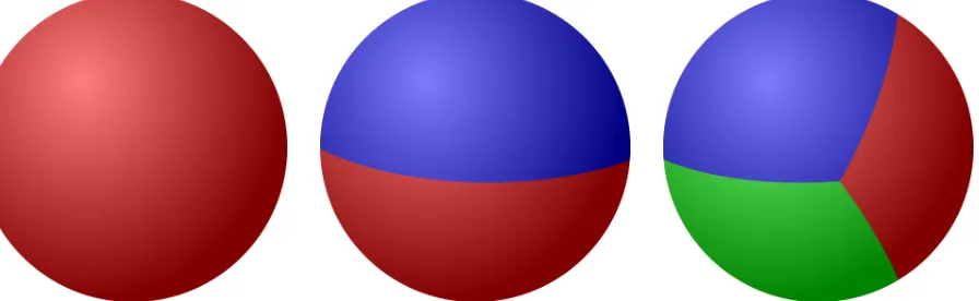
Figure 1: Plots of the known cases whenΓ is a sphere,m = 1 (left), m = 2 (center) andm = 3 (right) (Helffer et al. 2010).
i= 1, . . . , m, the collection of quasi-open sets{Γi}mi=1 is anm-partition ofΓwhich is a minimiser of (1.1) and
λ1(Γi) =
Z
Γ|∇Γ
ui|2 dσ fori= 1, . . . , m.
The authors Caffarelli and Lin (2007) use this formulation to show existence of minimisers and regularity of the interface between partitions.
Other works byConti, Terracini and Verzini (2002, 2003) and Caffarelli and Lin(2007, 2008) have focused on regularity and more qualitative aspects of the problem for a Cartesian domain. Conti, Terracini and Verzini derive optimality conditions, such as the gradient of eigenfunctions should match at partition boundaries, and also that the partition consists of open sets. Caffarelli and Lin obtain regularity results, such asC1,α-smoothness of the partition boundaries away from a set
of codimension two, and also an estimate of the behaviour in the limit of largem. In particular, they prove that the optimal energy is bounded above and below by a constant times themth eigenvalue onΓand conjecture that for largemthe optimal partition will be asymptotically close to a hexago-nal tiling in the case of a planar domain. The problem can be seen as a the strong competition limit of segregating species either in Bose-Einstein condensate (Chang, Lin, Lin and Lin 2004), popula-tion dynamics (Conti, Terracini and Verzini 2005a,b) and materials science (Chen 2002) in curved geometries.
The curved hypersurface problem has been studied analytically in the case thatΓis a sphere in recent work ofHelffer, Hoffmann-Ostenhof and Terracini(2010). They show the optimal partition is given by two hemispheres for the casem= 2and the so-called Y-partition form= 3; see Figure1 and section3.1. Furthermore, they show that for eachmthere is an optimal partition which satisfies an equal angle condition which says that the boundary arcs that meet at a critical point do so with equal angles.
Bozorgnia(2009). AlsoBourdin, Bucur and Oudet(2010) considered the problem for large values ofmusing a fictitious domain approach. This problem has also been considered on graphs (Coifman and Lafon 2006;Osting, White and Oudet 2014) with applications in big data segmentation. Finally, we mention the study which will be the basis of our work in the paper: an eigenfunction segregation approach (Du and Lin 2009). We will describe the algorithm in more detail in the following.
We derive computational approaches using the surface finite element method (Dziuk 1988;Dziuk and Elliott 2007) to find solutions to these problems. A review of computational techniques for partial differential equations on surfaces is given byDziuk and Elliott(2013). Our methods will be one of the algorithms given byDu and Lin(2009) applied with the surface finite element method in order to explore Problem1.1.
We believe some of the techniques used in this paper, such as operator splitting and parallel com-puting, could be applied in a wide range of multiphase problems; for example Gr¨aser, Kornhuber and Sack(2014). In these problems, one typically has a large system of reaction diffusion systems to solve with small parameter ε indicating an interfacial width. The small parameter ε acts with nonlinear terms to separate different phases. Our methods are designed to be transferable to this type of problem also. In contrast to many multiphase problems, the dynamic problem considered in this paper are based on non-local interface motion.
1.1
Approximation approach
One could try to directly compute the gradient flow of the energyESEG0 in (1.2); seeMayer(1998) for analytic considerations of this approach. However, this would lead to equations which would be hard to discretise. We instead relax the constraint thatutakes values inΞby adding a penalty term to the energy functional followingCaffarelli and Lin(2008). In this way, we consider the extended energy functional:
Eε
SEG(uε) =
m X i=1 1 2 Z Γ|∇ uε i| 2 dσ+
Z
Γ
Fε(uε) dσ, Fε(uε) =
1 ε2 m X i=1 m X j=1
j6=i
(uε i)
2(uε j)
2.
Problem 1.3. Given a positive integerm, a smooth surfaceΓandε >0, finduε = (uε
1, . . . , uεm)∈
H1(Γ,Rm)withkuε
ikL2(Γ) = 1fori= 1, . . . , m, to minimise
Eε
SEG(u
ε ) = m X i=1 1 2 Z Γ|∇
uεi|
2 dσ+
Z
Γ
Fε(uε) dσ. (1.3)
We will now compute the gradient flow of this relaxed problem. We now seek a time dependent functionuε: Γ×
R+→Rmandλε: R+ →Rmsatisfying
∂tuεi = ∆Γuεi +λiuεi −
2
ε2 X
j6=i
(uεj)2
!
uεi onΓ×R+, fori= 1, . . . , m, (1.4a)
subject to the constraint Z Γ| uε i| 2
dσ = 1 fori= 1, . . . , m. (1.5) Here, we suppose that the initial condition partitionsΓand has unit norm:
u0 ∈H1(Γ,Ξ),
Z
Γ u0i
2
dσ = 1 fori= 1, . . . , m.
We remark thatu0
i ≥0impliesuεi ≥0fori= 1, . . . , m.
This gradient flow problem was studied byCaffarelli and Lin(2009) for Cartesian geometries. The proofs can be easily transferred onto surfaces. We recall their results stated on surfaces:
λεi(t) =
Z
Γ|∇
uεi|
2 + 2
ε2 X
j6=i
(uεj)2
!
(uεi)2dσ,
and
Eε
SEG(uε)≤
m
X
i=1
λεi(t) =E ε
SEG(uε) + 2 Z
Γ
Fε(uε) dσ.
Furthermore, they show thatEε
SEG(uε)is a monotone decreasing function of time foruεthe solution of (1.4). This implies the existence of a unique global strong solutionuε∈L∞(R
+, H1(Γ,Rm)for each ε > 0. Finally, they give estimates of interest when considering the sharp interface limit: Denoting byu¯εthe minimiser of theε-problem, for any0< t
1 < t2, we have Z t2
t1
Z
Γ
Fε(¯uε) dσdt→0 asε→0,
and that the limit of minimising functions as ε → 0, u¯ε converges strongly in H1(Γ×R
+) to a suitable weak solution of the constrained gradient flow of (1.2).
A key advantage of this approach is that we are trying to approximate smooth functions uε in
place of the domains Γi. The limiting function u∗ = (u∗1, . . . , u∗m), is the limit of uε as ε → 0
partitionsΓ so we can define Γi = {u∗i > 0} and u∗j = 0inΓj, j 6= i. We note also that setting
v∗
i := u∗i −
P
j6=iu∗j we haveΓi = {v∗i > 0}. A possible disadvantage of this method is that it is
not clear how to relate uε to a partition {Γ
i}whenε is fixed. Possibilities for definingΓεi include
Γε
i ={uεi > c(ε)}orΓεi ={viε>0}whereviε:=uεi −
P
j6=iu ε j.
1.2
Outline
2
Computational method
2.1
Discretisation
We start the discretisation by taking a polyhedral approximationΓhofΓ. We assume thatΓhconsists
of a shape regular triangulationThwherehis the maximal diameter of a simplex (triangle forn= 2)
inTh. We will denote by Nh the vertices of Γh and callΓh a triangulated surface. We suppose that
ΓhinterpolatesΓin the sense that the vertices of triangles ofΓhlie onΓ.
Over this triangulation, we define two continuous finite element spaces, a space of scalar valued functionsShand a space of vector valued functionsSh. These are given by
Sh ={χh ∈C(Γh) :χh|T is affine linear, for allT ∈ Th}
Sh ={ηh = (ηh1, . . . , ηhm)∈C(Γh;Rm) :ηih ∈Shfori= 1, . . . , m}.
We can directly formulate the discrete version of Problem1.3.
Problem 2.1. Given a positive integer m, a triangulated surface Γh and ε > 0, find uε,h =
(uε,h1 , . . . , uε,h
m )∈Shto minimise
ESEGε,h (u
ε,h ) = m X i=1 Z Γh ∇Γhu
ε,h i 2
dσh+
Z
Γh
Fε(uε,h) dσh. (2.1)
Our optimisation strategy will be to directly solve a discretisation of the gradient flow equations. Discretising in space first, we seek a time dependent finite element functionuε,h∈C1(R
+;Sh)and
λε,h: R
+ →Rmsatisfying||uε,hi ||2Γh = 1 i= 1,2, ....m,
Z
Γh
∂tuε,hi χh+∇Γhu
ε,h
i · ∇Γhχhdσh
= Z
Γh
λε,hi u ε,h i χh−
2
ε2 X
j6=i
(uε,hj )2
!
uε,hi χhdσh for allχh ∈Sh
uε,h(·,0) =uh,0.
(2.2)
Here,uh,0 = (uh,10, . . . , uh,0
m )is initial data inSh such that(u h,0
i )2(u h,0
j )2 = 0for alli, j = 1, . . . , m
withi6=j.
We discretise in time using a operator splitting strategy similar to a scheme proposed by Du and Lin(2009). At each time step, we first solve one step of the heat equation, then solve an ordi-nary differential equation for the nonlinear terms, and use a projection to deal with the Lagrange multiplier.
2.2
Computational method
Algorithm 2.2. Given ε > 0, a positive integer m, a time step τ > 0 and an initial condition uh0 = ((uh
1)0, . . . ,(uhm)0) ∈ Sh with (uhi)0(z)2(uhj)0(z)2 = 0 for all z ∈ Nh and i, j = 1, . . . , m
withi6=j, fork = 0,1,2, . . .,
1. Solve one time step of the heat equation for i = 1, . . . , m using implicit Euler. We wish to findu˜ε,h = (˜uε,h1 , . . . ,u˜ε,h
m )∈Sh
Z
Γh 1
τ u˜ ε,h i −(u
ε,h i )k
χh+∇Γhu˜
ε,h
i · ∇Γhχhdσh = 0 for allχh ∈Sh, i= 1, . . . , m.
2. Solve the nonlinear terms exactly as ordinary differential equation at each node. For all nodes
z ∈ Nh andi= 1, . . . , m, finduˆε,hi (z) : [tk, tk+1]→Rsuch that
d dt
ˆ
uε,hi (z)(t)
=− 1
ε2 X
j6=i
(˜uε,hj (z))2
! ˆ
uε,hi (z)(t), uˆ ε,h i (z)(t
k
) = ˜uε,hi (z).
3. Find the new solution(uε,h)k+1by normalising the final time solution(ˆuε,h1 (·)(tk+1), . . . ,uˆε,hm (·)(tk+1)):
(uε,hi (z))k+1 = ˆ
uε,hi (z)(tk+1)
uˆ
ε,h
i (·)(tk+1)
L2(Γ
h)
for allz ∈ Nh, i= 1, . . . , m.
Similarly toBao and Du (2004), one can show an energy decreasing property for this scheme. The method is the same as the scheme of Du and Lin(2009) except we exchange a Gauss-Seidel iteration in step 2 for a Jacobi iteration. The ordinary differential equation from step 2 can be solved exactly to give:
ˆ
uε,hi (z)(t
k+1) = ˜uε,h
i (z) exp −
τ ε2
X
j6=i
(˜uε,hj (z)(t))2
!
.
Using this solution, we write a more practical version of step 2 as 2. For each nodez ∈ Nh,
(a) Fori= 1, . . . , m, computeu˜ε,hi (z)2;
(b) FindS=Pm
i=1u˜
ε,h i (z)2;
(c) Fori= 1, . . . , m, computeuˆiε,h(z)(tk+1)by ˆ
uε,hi (z)(tk+1) = ˜uε,h
i (z) exp
−τ
ε2(S−u˜
ε,h i (z)2)
We stop the computation when the change in energy is less than10−6. In order to reduce the computational cost this is only calculated everyMτ iterations where0.1 =Mττ.
Since, in general, we do not know the configuration of the optimal domains, we initialise the computations with a random initial condition. We loop over the grid nodesz ∈ Nh and uniformly
at random choose one valuei∈ {1, . . . , m}and set(uh
0)(z)i = 1and(uh0)(z)j = 0forj 6= ithen
normalise each component, (uh
0)i, fori = 1, . . . , m, inL2(Γ). As a result the first linear solve for
Remark. In practice, we find this operator splitting method to be stable and efficient. If we dis-cretised (2.2) in time directly using the Lagrange multiplier, we would have the choice to take the Lagrange multiplier implicitly or explicitly. An implicit discretisation would leave a fully coupled system of equations to solve, which would not be so easily implemented using parallel high perfor-mance computing techniques. An explicit discretisation would imply a time step restriction based on the size of the maximum H1-semi norm of each component. We wish to start with a random initial condition in order to avoid local minima, however this has a very largeH1-semi norm which would give an unfeasible time step restriction. All three methods are considered for the flat problem in the time discrete-space continuous case byDu and Lin(2009).
2.3
Parallel computations
The algorithm has been formulated so that we can use high performance computing to implement the optimisation. The key idea is to store the solution overmparallel processors and perform most of the computations on a single processor. Communication between processors is kept to a minimum. We distribute the solution uε,h over m processors so that processori storesuε,hi . At each time
step, each processor performs one linear solve (step 1), one loop over all nodes communicating with all other nodes to perform the sum in step 2(b) (step 2), then one more loop over all nodes to normalise the solution (step 3). In particular, computing sum in step 2(b) over allj is more efficient then computing the sum over all otherj 6=i.
A similar approach was also taken to parallelisation byBourdin et al.(2010) who computed up to512partitions. Our approach performs very well form ≤32. At the moment we restricted to this number of partitions because we wish to have a meaningful number of elements in each partition. It is possible that one may gain efficiency by using an adaptive mesh refinement on the unstructured grids enabling sufficiently accurate computations with a larger number of partitions. This is left for future work.
All test cases were implemented using the Distributed and Unified Numerics Environment (DUNE) (Bastian, Blatt, Dedner, Engwer, Kl¨ofkorn, Ohlberger and Sander 2008b; Bastian, Blatt, Dedner, Engwer, Kl¨ofkorn, Kornhuber, Ohlberger and Sander 2008a). Matrices are assembled using the DUNE-FEM (Dedner, Kl¨ofkorn, Nolte and Ohlberger 2010) and solved using a conjugate gradient method preconditioned with algebraic multigrid Jacobi preconditioner from DUNE-ISTL (Blatt and Bastian 2007). Parallelisation is performed usingMPI. All visualisation is performed in ParaView (Henderson 2014). The code we have written for the simulations in this paper is available at
3
Results
3.1
Convergence tests for three partitions of the sphere
From the work ofHelffer et al.(2010), we know that the Y-partition is optimal in the casem= 3on the sphere. This corresponds (up to rotations of the sphere) toΓ1 ={0< ϕ <2π/3},Γ2{−2π/3<
ϕ <0}andΓ3 ={|ϕ|>2π/3}. We can compute that the first eigenfunctions are:
u1(θ, ϕ) = sin(32φ)(sinθ)
3
2 onΓ
1
u2(θ, ϕ) =−sin(32φ)(sinθ)
3
2 onΓ
2
u3(θ, ϕ) = sin(3|2φ|−π)(sinθ)
3
2 onΓ
3.
Each of these eigenfunctions has eigenvalue15/4.
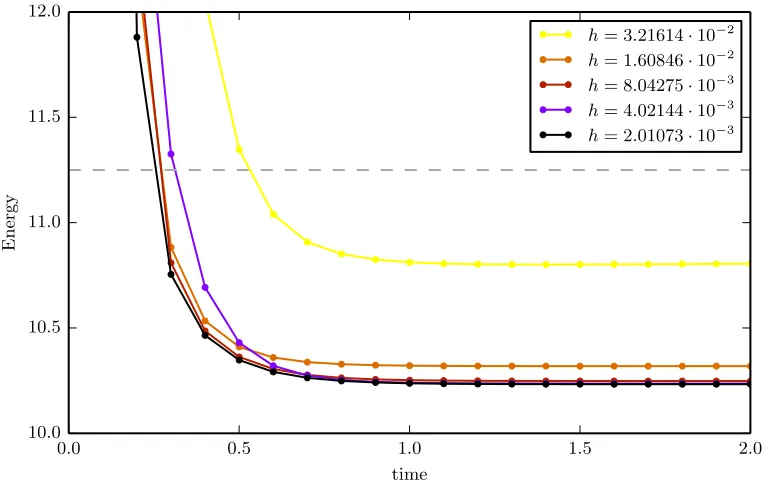
We first test convergence with respect to the discretisation parameters. We perform our algorithm atε= 5·10−3andτ = 10−4over five levels of mesh refinement, reducing fromh= 3.21614·10−2 toh= 2.01073·10−3. We compute untilt = 2. We have plotted the energy along the time evolution in Figure2and see good convergence. We have also included a dashed line at the exact energy45/4 forε= 0. We see that for a givenεthe error in energy can be large.
0.0 0.5 1.0 1.5 2.0
time 10.0
10.5 11.0 11.5 12.0
E
n
erg
y
h= 3.21614·10−2
h= 1.60846·10−
2
h= 8.04275·10−
3
h= 4.02144·10−
3
[image:10.612.94.479.416.660.2]h= 2.01073·10−3
Figure 2: Convergence with respect to discretisation parameters forε = 5·10−3 to the Y-partition on the sphere. The dashed grey line is the exact energy forε= 0.
ε Energy Energy error (eoc) Sε (eoc)
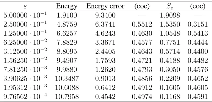
[image:11.612.126.464.92.255.2]5.00000·10−1 1.9100 9.3400 — 1.9098 — 2.50000·10−1 4.8759 6.3741 0.5512 1.5350 0.3151 1.25000·10−1 6.6257 4.6243 0.4630 1.0548 0.5413 6.25000·10−2 7.8829 3.3671 0.4577 0.7751 0.4444 3.12500·10−2 8.8095 2.4405 0.4643 0.5714 0.4400 1.56250·10−2 9.4907 1.7593 0.4721 0.4188 0.4482 7.81250·10−3 9.9880 1.2620 0.4793 0.3050 0.4576 3.90625·10−3 10.3487 0.9013 0.4856 0.2209 0.4652 1.95312·10−3 10.6088 0.6412 0.4912 0.1605 0.4605 9.76562·10−4 10.7958 0.4542 0.4974 0.1168 0.4591
Table 1: Results of convergence test inεfor numerical tests for three partition case. Energy isESEGε at the best computed partition, energy error is the difference to45/4the exact energy forε= 0, and
Sεis given by (3.1).
the mesh by bisecting elements once (two bisections reduceshroughly by half) and reduceτ by a factor1/√2. Instead of computing a new random initial condition after each refinement, we use the previous minimiser as the new initial condition.
We defineSεto be part of the energy associated with regularisation:
Sε(uε,h) :=
Z
Γh
Fε(uε,h) dσh =
1
ε2 Z
Γh
m
X
i=1 X
j6=i
(uε,hi )2(uε,hj )2dσh. (3.1)
These values illustrate the convergence of the relaxation to the exact problem. We expectSε →0as
we know that we recover the a minimiser of the partition problem asε →0.
We have computed the full and regularisation energy at each minimiser. The results are shown in Table1and Figure3. The tables also show the experimental order of convergence (eoc) which is computed via the formula
(eoc)i =
log(errori/errori−1) log(1/2) .
whereerrori is the error in energy against the exact partition at refinement leveli.
The eigenfunction segregation approach performs very well with respect to convergence in ε. We observe orderε12 convergence both for the full energy and also forS
ε. The errors are still quite
large for reasonable sized values ofεso we must take very small values ofεto trust any predictions of energy values using this method.
3.2
Computed partitions of the sphere for
m
≥
3
0 1 2 3 4 5 6 7 level
10−1
100 101
E
n
erg
y
erro
r
0 1 2 3 4 5 6 7
level 10−1
100 101
Sε
ε
[image:12.612.95.491.109.358.2]10−3 10−2 10−1
Figure 3: Convergence with respect toεto the Y-partition on the sphere. The energy error is differ-ence to45/4the exact energy forε= 0, andSεis given by (3.1).
τl+1 as
εl+1 = √
2εl τl+1 = √
2τl.
We use the optimal function for levell−1as the initial condition on levell. The final parameters are given in Table2.
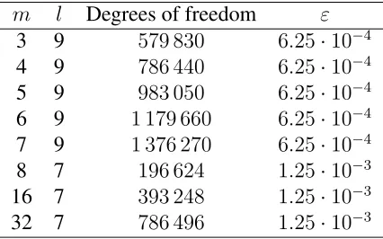
Plots of the solutions for several values of m are given in Figures 4. Observe that the colour coding of these figures indicates the partitions using the computed values of the eigenfunctions. Eigenvalue estimates are computing by taking the mean H1-semi norm of the components. The computed eigenvalues are plotted in Figure5. Theorem 3 of the work byCaffarelli and Lin(2007) proves that the energy scales likeλm(Γ)up to a constant factor. Using Weyl’s asymptotics, we see
m l Degrees of freedom ε
3 9 579 830 6.25·10−4 4 9 786 440 6.25·10−4 5 9 983 050 6.25·10−4 6 9 1 179 660 6.25·10−4 7 9 1 376 270 6.25·10−4 8 7 196 624 1.25·10−3 16 7 393 248 1.25·10−3 32 7 786 496 1.25·10−3
[image:12.612.188.401.590.723.2]that in two space dimensions this means that the average eigenvalue is bounded above and below by m times a constant. This is indicated by the blue line which is m times the first eigenvalue corresponding to a hexagonH of area4π(the surface area of the sphere) – this is the conjectured average eigenvalue for largemin the plane (Caffarelli and Lin 2007). Our results indicate a similar scaling property for the sphere.
Rather than just using the computed eigenfunction values, as mentioned earlier, we may define an approximate partition by
Γε,hi := (
x∈Γ :viε,h(x) :=uε,hi (x)−X
j6=i
uε,hj (x)>0 )
fori= 1, . . . , m. (3.2)
We motivate the use of this definition by noting that eachuε,hi is positive and the supports of{uε,hi }
overlap, hence this function is zero only surrounding one partition whereuε,hi =u ε,h
j for somej 6=i.
Note that these sets will not coverΓ and there will be a small void between regions. Furthermore we may useviε,hin the following interesting way. Suppose thatγ is a curve onΓdefined by as the zero level set of a functionφ,γ = {φ = 0}, then the geodesic curvature ofγ, which we denote by
κg is given by
κg =∇Γ·
∇Γφ |∇Γφ|
. (3.3)
We can use ParaView’s gradient reconstruction function to compute an approximation ofκg over
the interface at the boundary of each partitionΓi usingφ = vε,hi . An example of this is shown in
Figure6. We see that this value is small away from junctions.
We observe that at junctions three partitions coincide with equal angles. See, for example, Fig-ure7. This is consistent with the results ofHelffer et al. (2010) who prove that all partitions have an equal angle property. From our results it is difficult to quantify this result since at any triple point there is a void region because of our regularisation. Also in Figure7, we have superimposed an equal angle triple junction which shows good agreement to results we have. We can consider a reduced problem of finding the first eigenvalue over partitions of the unit disk. We find with three equal partitions (similar to the Y-partition) the total energy is approximately60.6(= 3·20.2)and for four partitions, one in each quadrant, the total energy is approximately105.6(= 4·26.4). Taking three partitions leads to a significant reduction in energy.
Table 3shows one representative of each polygon similarity class and more details of the best estimate of the energy and also the similarity classes of polygons. The energy calculation shows the values of each eigenvalue (mean and standard deviation for each similarity class of polygons) and alsoSεfor each of the final configurations.
There are several striking features:
• All partitions consist of curvi-linear polygons;
(a)m= 3, 3 lens (pink) (b)m= 4, 4 triangles (red)
(c)m = 5, 2 triangles (red) and
3 quadrilaterals (orange)
(d)m = 6, 6 quadrilaterals
(or-ange)
(e) m = 7, 5 quadrilaterals
(or-ange) and 2 pentagons (yellow)
(f) m = 8, 4 quadrilaterals
(or-ange) and 4 pentagons (yellow)
(g) m = 16, 8 A and 4 B
pen-tagons (yellow) and 4 hexagons (green)
(h)m = 32, 12 pentagons
[image:14.612.58.535.118.663.2](yel-low) and 20 hexagons (green)
Figure 4: Plots of the minimising configurations{Γε,hi }m
100
101
102
m
100 101 102
E
ig
en
va
lu
e
[image:15.612.122.458.133.343.2]mλ1(H)
Figure 5: Plot of the eigenvalues at different values ofm. The blue line ismλ1(H)whereH is the planar hexagon with area4π (equal to the surface area of the sphere).
Figure 6: Plots of one partition and κg form = 8(left) and m = 16 (right). The value ofuε,hi is
shown on a black to white scale andκgis plotted on the curve{v ε,h
[image:15.612.104.484.454.674.2]m Shape Energy information
3
3 lens
Lens eigenvalue:3.605 (2.59·10−4)
Sε:0.072
Total energy:10.887
4
4 triangles
Triangle eigenvalue:4.966 (2.46·10−4)
Sε:0.121
Total energy:19.987
5
2 triangles
and
3 quadrilaterals
Triangle eigenvalue:7.118 (3.35·10−4) Quadrilateral eigenvalue:6.302
Sε:0.187
Total energy:33.330
6
6 quadrilaterals
Quadrilateral eigenvalue:7.812 (7.22·10−4)
Sε:0.248
Total energy:47.122
7
5 quadrilaterals
and
2 pentagons
Quadrilateral eigenvalue:9.988 (1.63·10−3) Pentagon eigenvalue:8.298 (7.50·10−5)
Sε:0.322
Total energy:66.859
8
4 quadrilaterals
and
4 pentagons Quadrilateral eigenvalue: 11.380 (5.31·10−3)
Pentagon eigenvalue:10.230 (2.91·10−3)
Sε:0.650
Total energy:87.102
16
8 A and 4 B pentagons
and
4 hexagons
Pentagon (A) eigenvalue: 22.647 (1.05·10−2) Pentagon (B) eigenvalue:
23.610 (2.43·10−2)
Hexagon eigenvalue:20.496 (1.05·10−2)
Sε:1.264
Total energy:362.718
32
12 pentagons
and
20 hexagons
Pentagon eigenvalue:48.436 (1.46·10−1) Hexagon eigenvalue:44.460 (1.24·10−1)
Sε:2.496
[image:16.612.56.572.90.721.2]Total energy:1472.920
Table 3: More details of optimal partitions. In the small plots, we plot the correspondinguε,hi with a
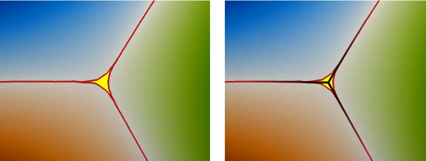
Figure 7: A zoom of a triple junction on the sphere. Three partitions{vε,hi > 0} are coloured on blue, green and orange according to the eigenfunctionuε,hi with red boundaries at {v
ε,h
i = 0}. The
void region is shown in yellow. Additionally in the right plot we have added black lines which would correspond to an equal angle triple junction.
• Each junction is a triple junction with an equal angle condition satisfied;
• There are at most two types of polygon in the partition;
• In the case of two different polygons, the polygon with more sides has lower eigenvalue;
• Asmincreases the number of edges in each polygon increases;
• Each polygon has at most6edges.
We define the dual polygon to a partition by considering the edges and vertices as a graph and taking the dual graph. In our case, since we always have triple junctions this defines a triangulation of the sphere. LetV be the number of vertices,Ethe number of edges andF the number of faces in the dual polygon to a partition{Γi}mi=1. We know that this will satisfy Euler’s identity,V −E+F =
χ, whereχis the Euler characteristic (2in the case of a sphere), and also that
2E = ∞ X
k=0
knk, 3F =
∞ X
k=0
knk, V =
∞ X
k=0
nk,
wherenkis the degree of a vertex in the dual polygon. The degree of a vertex is equal to the number
of edges of the corresponding partition. Using these equations in Euler’s identity gives
4n2+ 3n3+ 2n4+n5 = 6χ+ ∞ X
k=7
(k−6)nk. (3.4)
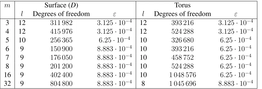
m Surface (D) Torus
l Degrees of freedom ε l Degrees of freedom ε
[image:18.612.81.516.93.241.2]3 12 311 982 3.125·10−4 12 393 216 3.125·10−4 4 12 415 976 3.125·10−4 12 524 288 3.125·10−4 5 10 256 365 6.25·10−4 10 326 680 6.25·10−4 6 9 150 900 8.883·10−4 10 393 216 6.25·10−4 7 9 176 050 8.883·10−4 10 458 752 6.25·10−4 8 9 201 200 8.883·10−4 10 524 288 6.25·10−4 16 9 402 400 8.883·10−4 10 1 048 576 6.25·10−4 32 9 804 800 8.883·10−4 8 1 045 696 8.883·10−4
Table 4: Final parameters for computations on the other surfaces (D) and the torus.
correspond to zero Gauss curvature and polygons with more than six sides correspond to negative Gauss curvature.
This identity is consistent with the partitions in Table 3. Our computations suggest that the polygonal structure of the optimal partition consists of polygons with six or less sides. This agrees with the idea that the sphere has uniform positive Gauss curvature. We can deduce that if anm -partition of the sphere consists of only pentagons and hexagons, then there will be12pentagons and
m−12hexagons. We expect this to be the optimal partition for large values ofm.
3.3
Computed partitions of other surfaces
We consider two other surfaces to see if these conclusions persist on a large class of surfaces. The first example, surface (D), is taken from the work of Dziuk (1988) where the surface is given by Γ ={x∈R3 : Φ(x) = 0}forΦgiven by
Φ(x1, x2, x3) := (x1−x32)2+x22+x23−1.
This has the same genus as a sphere but has large changes in curvature. The second example is given by a torus (T) with inner radius0.6and outer radius 1. This has different genus to the sphere. We proceed with the same refinement strategy as on the sphere. Details of the parameters is given in Table4.
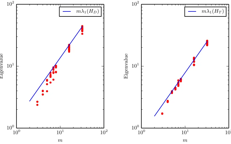
We plot for the eigenvalues corresponding to the optimal partition Figure 8. We compute the eigenvalue as theH1(Γ)semi-norm of each component. We have also included the line atmλ
1(HD)
and mλ1(HT) in each plot, where HD and HT are the regular hexagons with area equal to the
surfaces of example 1 (D) and the torus (T). We do not have direct access to the eigenvalues on either of these surfaces so do not add that to this plot.
100
101
102
m
100 101 102
E
ig
en
va
lu
e
mλ1(HD)
100
101
102
m
100 101 102
E
ig
en
va
lu
e
[image:19.612.96.490.261.506.2]mλ1(HT)
(a)m= 3, 3 lens (pink) (b)m= 4, 4 triangles (red)
(c)m = 5, 2 triangles (red) and
3 quadrilaterals (orange)
(d)m = 6, 6 quadrilaterals
(or-ange)
(e) m = 7, 5 quadrilaterals
(or-ange) and 2 pentagons (yellow)
(f) m = 8, 4 quadrilaterals
(or-ange) and 4 pentagons (yellow)
(g)m = 16, 3 quadrilateral
(or-ange), 6 pentagons (yellow), 7 hexagons (green)
(h)m = 32, 12 pentagons
[image:20.612.56.536.139.658.2](yel-low) and 20 hexagons (green).
(a)m= 3, 3 cylinders (grey) (b)m= 4, 4 cylinders (grey)
(c) m = 5, 4 two-sided shapes
(pink) and 1 quadrilateral (or-ange)
(d)m= 6, 6 hexagons (green)
(e) m = 7, 2 quadrilaterals
(orange), 2 pentagons (yellow), 1 hexagon (green), 1 octagon (blue), 1 decagon (purple)
(f)m= 8, 4 pentagons (yellow),
1 hexagon (green), 2 heptagons (cyan), 1 octagon (blue)
(g) m = 16, 2
quadrilater-als (orange), 4 pentagons (yel-low), 8 hexagons (green) and 2 decagons (purple)
(h) m = 32, 8 pentagons
[image:21.612.65.534.89.689.2](yel-low), 18 hexagons (green), 4 heptagons (cyan) and 2 octagons (blue).
m Partition
3
lens
2.664
crescent
2.664
crescent
2.372
Sε:0.040
Total energy:7.741
4
triangle
3.493
triangle
3.494
triangle
4.008
triangle
3.952
Sε:0.103
Total energy:15.051
5
triangle
5.843
triangle
5.125
quadrilateral
6.004
quadrilateral
5.944
quadrilateral
3.942
Sε:0.312852
Total energy:27.072
6
quadrilateral
7.808
quadrilateral
7.241
quadrilateral
7.093
quadrilateral
6.753
quadrilateral
6.730 quadrilateral
5.443
Sε:0.753
7
quadrilateral
9.569
quadrilateral
9.556
quadrilateral
9.275
quadrilateral
8.748
quadrilateral
7.780 pentagon
8.009
pentagon
6.058
Sε:1.102
Total energy:60.096
8
quadrilateral
10.1602
quadrilateral
9.83384
quadrilateral
8.09237
quadrilateral
7.978 pentagon
10.128
pentagon
10.034
pentagon
9.965
pentagon
9.539
Sε:1.63602
[image:23.612.59.557.175.626.2]Total energy:77.367
Table 5: More details of optimal partitions. In the small plots, we plot the correspondinguε,hi with a
m Partition
3
cylinder
1.725
cylinder
1.703
cylinder
1.717
Sε:1.207
Total energy:6.353
4
cylinder
2.758
cylinder
2.637
cylinder
2.595
cylinder
2.595
Sε:0.106
Total energy:10.890
5
two sided shape
3.772
two sided shape
3.940
two sided shape
3.683
two sided shape
3.914
quadrilateral
3.812
Sε:0.595
Total energy:19.717
6
hexagon
4.215
hexagon
4.481
hexagon
4.319 hexagon
4.319
hexagon
4.480
hexagon
4.215
Sε:1.005
7
quadrilateral
4.803
quadrilateral
5.064
pentagon
5.168
pentagon
4.94272 hexagon
5.465
octagon
5.459
decagon
5.908
Sε:0.81257
Total energy:37.623
8
pentagon
5.951
pentagon
5.841
pentagon
6.070
pentagon
6.105 hexagon
5.692
heptagon
6.186
heptagon
6.184
octagon
6.254
Sε:1.257
[image:25.612.58.557.174.622.2]Total energy:49.540
Table 6: More details of optimal partitions. In the small plots, we plot the correspondinguε,hi with a
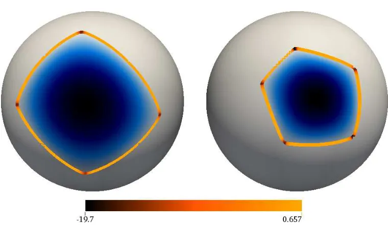
By usingΓε,hi andv ε,h
i from (3.2), we can define the boundary of partition on these surfaces also.
This allows us to compute the geodesic curvature (3.3) of the boundary of Γε,hi ; see Figure11for
computations. We again see that away from junctions the geodesic curvature is small. We also see that boundaries all meet at triple junction with the equal angle condition satisfied. We conjecture that on all surfaces optimal partitions have boundaries with zero geodesic curvature which meet at triple junctions with equal angles between each boundary.
On surface (D), the partition has exactly the same structure as for the sphere form ≤ 8but the eigenvalues do not group in the same way because of the variations in curvature. For large values ofm the structure changes. Now in regions with higher curvature we see partitions with few sides. In fact, form = 16, three partitions have four sides, which does not occur in the case of the sphere. The familiar pattern of pentagons and hexagons reoccurs form = 32except now the pentagons are clustered in regions of high curvature. The number of sides of each partition is still limited to six. Because of (3.4), for larger values ofm we expect to see12pentagons andm−12hexagons with the pentagons clustered in the higher curvature regions.
On the torus, example (T), the situation is very different. Form ≤ 6, we have very structured partitions which reflect the symmetry of the surface. For the case of m = 5, we see all triple junctions occur in the center of the torus. Form > 6, we have partitions with more that 6sides. The formula (3.4) tells us that the numbers of partitions with more than six sides must balance the number of partitions with less than six sides. For the cases we see, the partitions with more than six sides cluster in the center and those with less than six sides cluster on the exterior. As we increasem
the see an increase in the number of hexagons, and it is not clear whether the number of partitions with different to six sides will decrease. For smaller area partitions, for largerm, the curvature of the surface is less important and the problem becomes more like the flat problem, so we expect that for large values ofm, we will see a preponderance of hexagons.
4
Discussion
We have explored an eigenvalue partition problem on three different surfaces and for many differ-ent numbers of partitions. We have observed good convergence both with respect to discretisation parameters and also with respect to our choice of regularisation. From our results we make the following conjectures:
1. The optimal partition consists of curvilinear polygons whose edges have zero geodesic cur-vature.
2. Partitions either meet along edges or at triple junctions where edges meet at equal angles. 3. For genus zero surfaces, for large values ofm the optimal partition consists of12pentagons
Figure 11: Plots of one partition andκg form = 8for Example 1 (left) andm = 6for Example 2
(right). The value ofuε,hi is shown on a black to white scale andκgis plotted on the curve{v ε,h i = 0}
on a black to orange scale.
4. For genus one surfaces, for large values of m the optimal partition has a preponderance of hexagons.
Acknowledgments
The research of TR was funded by the EPSRC (grant number EP/L504993/1). This work was un-dertaken on ARC2, part of the High Performance Computing facilities at the University of Leeds. The authors were participants of the Isaac Newton Institute programme Free Boundary Problems and Related Topics (January–July 2014) when this article was written.
References
Bao, W. and Du, Q. Computing the ground state solution of Bose–Einstein condensates by a nor-malized gradient Flow. SIAM J. Sci. Comput., 25(5):1674–1697, 2004.
Bastian, P., Blatt, M., Dedner, A., Engwer, C., Kl¨ofkorn, R., Kornhuber, R., Ohlberger, M., and Sander, O. A generic grid interface for parallel and adaptive scientific computing. Part II: imple-mentation and tests in DUNE. Comput., 82(2–3):121–138, 2008a.
generic grid interface for parallel and adaptive scientific computing. Part I: abstract framework.
Comput., 82(2–3):103–119, 2008b.
Blatt, M. and Bastian, P. The iterative solver template library. InProceedings of the 8th international conference on Applied parallel computing: state of the art in scientific computing, PARA’06, pages 666–675, Berlin / Heidelberg, 2007. Springer-Verlag.
Bonnaillie-No¨el, V., Helffer, B., and Vial, G. Numerical simulations for nodal domains and spectral minimal partitions. ESAIM: Control Optim. Calc. Var., 16:221–246, 1 2010.
Bourdin, B., Bucur, D., and Oudet, E. Optimal partitions for eigenvalues. SIAM J. Sci. Comput., 31 (6):4100–4114, 2010.
Bozorgnia, F. Numerical algorithm for spatial segregation of competitive systems. SIAM J. Sci. Comput., 31(5):3946–3958, 2009.
Bozorgnia, F. and Arakelyan, A. Numerical algorithms for a variational problem of the spatial segregation of reaction–diffusion systems. Appl. Math. Comput., 219(17):8863 – 8875, 2013.
Bucur, D. and Zolesio, J. N-dimensional shape optimization under capacitary constraint. J. Differ. Equations, 123(2):504 – 522, 1995.
Bucur, D., Buttazzo, G., and Henrot, A. Existence results for some optimal partition problems.Adv. Math. Sci. Appl., 8:571–579, 1998.
Buttazzo, G. and Dal Maso, G. An existence result for a class of shape optimization problems.Arch. Ration. Mech. An., 122(2):183–195, 1993.
Caffarelli, L. and Lin, F. An optimal partition problem for eigenvalues. J. Sci. Comput., 31(1-2): 5–18, 2007.
Caffarelli, L. and Lin, F. Singularly perturbed elliptic systems and multi-valued harmonic functions with free boundaries. J. Am. Math. Soc., 21(3):847–862, 2008.
Caffarelli, L. and Lin, F. Nonlocal heat flows preserving theL2 energy. Discrete Cont. Dyn. – A, 23:49–64, 2009.
Chang, S. M., Lin, C. S., Lin, T. C., and Lin, W. W. Segregated nodal domains of two-dimensional multispecies Bose-Einstein condensates. Phys. D., 196(3–4):341–361, 2004.
Chen, L.-Q. Phase-field models for microstructure evolution. Annu. Rev. Mater. Res., 32:113–140, 2002.
Conti, M., Terracini, S., and Verzini, G. Nehari’s problem and competing species systems. Ann. I. H. Poincar´e – AN, 19(6):871 – 888, 2002.
Conti, M., Terracini, S., and Verzini, G. An optimal partition problem related to nonlinear eigenval-ues. J. Funct. Anal., 198(1):160 – 196, 2003.
Conti, M., Terracini, S., and Verzini, G. Asymptotic estimates for the spatial segregation of com-petitive systems. Adv. Math., 195(2):524 – 560, 2005a.
Conti, M., Terracini, S., and Verzini, G. A variational problem for the spatial segregation of reaction-diffusion systems. Indiana Univ. Math. J., 54:779–816, 2005b.
Dedner, A., Kl¨ofkorn, R., Nolte, M., and Ohlberger, M. A generic interface for parallel and adaptive discretization schemes: abstraction principles and the DUNE-FEM module. Comput., 90(3-4): 165–196, 2010.
Du, Q. and Lin, F. Numerical approximations of a norm-preserving gradient flow and applications to an optimal partition problem. Nonlin., 22(1):67, 2009.
Dziuk, G. Finite Elements for the Beltrami operator on arbitrary surfaces. In Hildebrandt, S. and Leis, R., editors,Partial Differential Equations and Calculus of Variations, volume 1357 of
Lecture Notes in Mathematics, pages 142–155. Springer-Verlag, Berlin, 1988.
Dziuk, G. and Elliott, C. M. Surface finite elements for parabolic equations.J. Comp. Math., 25(4): 385–407, 2007.
Dziuk, G. and Elliott, C. M. Finite element methods for surface PDEs. Acta Numer., 22:289–396, 2013.
Gr¨aser, C., Kornhuber, R., and Sack, U. Nonsmooth Schur–Newton methods for multicomponent Cahn–Hilliard systems. IMA Journal of Numerical Analysis, 2014.
Helffer, B., Hoffmann-Ostenhof, T., and Terracini, S. On spectral minimal partitions: the case of the sphere. In Laptev, A., editor, Around the Research of Vladimir Maz’ya III, volume 13 of
International Mathematical Series, pages 153–178. Springer New York, 2010.
Henderson, A. ParaView: Parallel visualization application (Version 4.1.0) [Computer Software]. Available athttp://www.paraview.org, 2014.
Mayer, U. F. Gradient flows on nonpositively curved metric spaces and harmonic maps. Commun. Anal. Geom., 6(2):199–253, 1998.
Osting, B., White, C. D., and Oudet, E. Minimal Dirichlet energy partitions for graphs. arXiv, 1308.4915, 2014.