Particle Approximations of the Score and Observed Information Matrix for Parameter Estimation in State Space Models With Linear Computational Cost

White Rose Research Online URL for this paper: http://eprints.whiterose.ac.uk/92279/

Version: Accepted Version

Article:

Nemeth, C., Fearnhead, P. and Mihaylova, L.S. (Accepted: 2015) Particle Approximations of the Score and Observed Information Matrix for Parameter Estimation in State Space Models With Linear Computational Cost. Journal of Computational and Graphical Statistics. ISSN 1061-8600

https://doi.org/10.1080/10618600.2015.1093492

[email protected] https://eprints.whiterose.ac.uk/

Reuse

Unless indicated otherwise, fulltext items are protected by copyright with all rights reserved. The copyright exception in section 29 of the Copyright, Designs and Patents Act 1988 allows the making of a single copy solely for the purpose of non-commercial research or private study within the limits of fair dealing. The publisher or other rights-holder may allow further reproduction and re-use of this version - refer to the White Rose Research Online record for this item. Where records identify the publisher as the copyright holder, users can verify any specific terms of use on the publisher’s website.

Takedown

If you consider content in White Rose Research Online to be in breach of UK law, please notify us by

Particle Approximations of the Score and Observed

Information Matrix for Parameter Estimation in State

Space Models With Linear Computational Cost

Christopher Nemeth, Paul Fearnhead and Lyudmila Mihaylova

Abstract

Poyiadjis et al. (2011) show how particle methods can be used to estimate both the score

and the observed information matrix for state space models. These methods either suff_{er from}

a computational cost that is quadratic in the number of particles, or produce estimates whose

variance increases quadratically with the amount of data. This paper introduces an alternative

approach for estimating these terms at a computational cost that is linear in the number of

parti-cles. The method is derived using a combination of kernel density estimation, to avoid the

par-ticle degeneracy that causes the quadratically increasing variance, and Rao-Blackwellisation.

Crucially, we show the method is robust to the choice of bandwidth within the kernel density

estimation, as it has good asymptotic properties regardless of this choice. Our estimates of the

score and observed information matrix can be used within both online and batch procedures

for estimating parameters for state space models. Empirical results show improved parameter

estimates compared to existing methods at a significantly reduced computational cost.

Supple-mentary materials including code are available.

Keywords. Gradient ascent algorithm; Maximum likelihood parameter estimation; Particle

filter-ing; Sequential Monte Carlo; Stochastic approximation

Christopher Nemeth, Department of Mathematics and Statistics, Lancaster University, Lancaster LA1 4YF, UK (Email: [email protected]). Paul Fearnhead, Department of Mathematics and Statistics, Lancaster University, Lancaster LA1 4YF, UK (Email: [email protected]). Lyudmila Mihaylova, Department of Automatic Con-trol and Systems Engineering, University of Sheffi_{eld, She}ffi_{eld S1 3JD, UK (Email: l.s.mihaylova@she}ffi_eld.ac.uk).

1

Introduction

State space models have become a popular framework to model nonlinear time series problems

in engineering, econometrics and statistics (Capp´e et al., 2005; Durbin and Koopman, 2001). In

this paper we consider the problem of maximum likelihood estimation of the model parameters,θ,

for nonlinear, non-Gaussian state space models, where there is no closed form expression for the

marginal likelihood, p(y1:T|θ), for data y1:T = {y1,y2, . . . ,yT}.

Using sequential Monte Carlo (SMC) methods, also known as particle filters, we propose an

effi_{cient method to create particle approximations of the score vector∇log p(y1:T|θ), which can be}

used within a gradient ascent algorithm to estimateθby indirectly maximising the likelihood

func-tion. We show that our proposed algorithm can be applied offl_{ine, to estimate theθfrom batches of}

data, or recursively, to updateθwhen new observations ytare received. Previous work by Poyiadjis

et al. (2011), has provided two approaches for estimating the score vector and observed

informa-tion matrix. The first has a computainforma-tional complexity that is linear in the number of particles, but

it has the drawback that the variance of the estimates increases quadratically through time. The

second method produces estimates whose variance increases linearly with time, but at the expense

of a computational cost that is quadratic in the number of particles. The increased computational

complexity of this algorithm limits its use for online applications.

We propose a new method for estimating the score vector and observed information matrix

using a novel implementation of a kernel density estimation technique (Liu and West, 2001), with

Rao-Blackwellisation to reduce the Monte Carlo error of our estimates. The result is a linear-time

algorithm which has substantially smaller Monte Carlo variance than the linear-time algorithm of

Poyiadjis et al. (2011) and notable improvements over the fixed-lag smoother (Olsson et al., 2008)

– with empirical results showing the Monte Carlo variance of the estimate of the score vector

increases only linearly with time. Furthermore, unlike standard uses of kernel density estimation,

we derive results showing that our method is robust to the choice of bandwidth. For any fixed

bandwidth our approach can consistently estimate the parameters as both the number of

time-points and the number of particles go to infinity.

Our final algorithm has similarities with the fixed-lag smoother of Dahlin et al. (2014), in terms

of reducing the Monte Carlo error in the score and observed information estimates. However, one

of the key advantages of our approach using Rao-Blackwellisation and kernel density estimation is

that we are able to better approximate the observed information matrix, which in turn leads to faster

and more accurate parameter estimation. A recently proposed linear time algorithm by Westerborn

and Olsson (2014), supported by theoretical results (Olsson and Westerborn, 2014), could be also

be used, but is not tested here. Finally, compared to competing methods, empirical results on a

challenging eight parameter nonlinear model show that our algorithm produces more consistent

parameter estimates, with an order of magnitude improvement in the rate of convergence.

2

Inference for state space models

2.1

State space models

Consider the general state space model where _{Xt; 1 ≤ t ≤ T}represents a latent Markov process

that takes values on _{X ⊆} Rnx_{. The process is fully characterised by its initial density p(x}

1|θ) =

μθ(x1) and transition probability density

p(xt|x1:t−1, θ)= p(xt|xt−1, θ)= fθ(xt|xt−1), (1)

whereθ _∈ Θ_{represents a vector of model parameters. For an arbitrary sequence{zi}the notation}

zi: jcorresponds to (zi,zi+₁, . . . ,z_j) for i≤ j.

We assume that the process _{Xt} is not directly observable, but partial observations can be

made via a second process _{Yt; 1 ≤ t ≤ T} ⊆ Y ⊆ Rny. The observations {Yt} are conditionally

independent given_{Xt}and are defined by the probability density

p(yt|y1:t−1,x1:t, θ)= p(yt|xt, θ)=gθ(yt|xt). (2)

In the standard Bayesian context the latent process_{X1:T}is estimated conditional on a sequence

of observations y1:T, for T ≥1. If the parameter vectorθis known then the conditional distribution

p(x1:T|y1:T, θ)∝ p(x1:T,y1:T, θ) can be evaluated where

p(x1:T,y1:T, θ)= μθ(x1)

T Y

t=₂

fθ(xt|xt−1)

T Y

t=₁

gθ(yt|xt). (3)

For nonlinear, non-Gaussian state space models it is not possible to evaluate the posterior

den-sity p(θ,x1:T|y1:T) in closed form. A popular approach for approximating these densities is to use a

sequential Monte Carlo algorithm.

2.2

Sequential Monte Carlo algorithm

SMC algorithms allow for the sequential approximation of the conditional density of the latent

state given a sequence of observations, y1:t, for a fixed θ, which in this section we assume are

known model parameters. For simplicity we shall focus on methods aimed at approximating the

conditional density for the current state, Xt, but the ideas can be extended to learning about the full

path of the process, X1:t. Approximations of the density p(xt|y1:t, θ) can be calculated recursively

by first approximating p(x1|y1, θ), then p(x2|y1:2, θ) and so forth. Each conditional density can be

approximated by a set of N weighted random samples, called particles, where

ˆp(dxt|y1:t, θ)=

N X

i=₁

w(i)_t δ_X(i)

t (dxt), ∀i w

(i)

t ≥0, N X

i=₁

w(i)_t =_{1 (4)}

is an approximation for the conditional distribution and δx0(dx) is a Dirac delta mass function

located at x0. The set of particles{Xt(i)}Ni=₁and their corresponding weights{w

(i)

t }iN=₁ provide an

em-pirical measure that approximates the probability density function p(xt|y1:t, θ), where the accuracy

of the approximation increases as N _{→ ∞}(Crisan and Doucet, 2002).

We can recursively update our approximation using the following filtering recursion,

p(xt|y1:t, θ)∝ gθ(yt|xt) Z

fθ(xt|xt−1)p(xt−1|y1:t−1, θ)dxt−1, (5)

where if we assume that at time t ₋1 we have a set of particles _{X_t(i)_−1}N

i=₁, and weights {w

(i)

t−1}

N i=₁,

which produce a discrete approximation to p(x_t−1|y1:t−1, θ), we can then create a Monte Carlo

ap-proximation for (5) as

p(xt|y1:t, θ)≈ cgθ(yt|xt) N X

i=₁

w(i)_t−1fθ(xt|x

(i)

t−1), (6)

where c is a normalising constant. Particle approximations as given above can be updated

recur-sively by propagating and updating the particle set using importance sampling techniques. There

is now an extensive literature on particle filtering algorithms, see for example, Doucet et al. (2000)

and Capp´e et al. (2007).

In this paper the particle approximations of the latent process are created with the auxiliary

particle filter of Pitt and Shephard (1999). This filter has a general form, and simpler filters can

be derived as special cases (Fearnhead, 2007). The idea is to approximate cw(i)_t−1gθ(yt|xt) fθ(xt|x

(i)

t−1)

withξ(i)_t q(xt|x(i)_t−1,yt, θ), for a set of probabilitiesξt(i)and proposal densities q(xt|x(i)_t−1,yt, θ). We

simu-late particles at time t by first choosing a particle at time t ₋1, with particle x(i)_t−1 being chosen with probability ξ_t(i). We then propagate this to time t by sampling our particle at time t, xt,

from q(xt|x(i)_t−1,yt, θ). The importance sampling weight assigned to our new particle x(i)t is then w(i)_t−1gθ(yt|xt) fθ(xt|x_t−(i)₁)/ξ(i)t q(xt|x(i)_t−1,yt, θ). Details are summarised in Algorithm 1.

Algorithm 1 Auxiliary Particle Filter Step 1: iteration t= _1.

Sample_{x(i)_{1 }}from the prior p(x1|θ), set and normalise weights w(i)₁ = gθ(y1|x(i)₁ ).

Step 2: iteration t= _{2, . . . ,T .}

Assume a set of particles_{x(i)_t−1}N

i=₁and associated weights{w

(i)

t−1}

N

i=₁that approximate p(xt−1|y1:t−1, θ)

and user-defined set of proposal weights_{ξ_t(i)_}N_i=₁and family of proposal densities q(∙|xt−1,yt, θ).

(a) Sample indices_{k1,k2, . . . ,kN}from{1, . . . ,N}with probabilitiesξ(i)t .

(b) Propagate particles x(i)_{t ∼}q(_∙|x(ki)

t−1,yt, θ).

(c) Weight each particle w(i)_{t ∝} w(ki)t−1gθ(yt|x (i)

t ) fθ(x(i)t |x(ki)t−1)

ξ(ki)_t q(x(i)_t |x(ki)_t−1,yt,θ) and normalise the weights.

3

Parameter estimation for state space models

3.1

Maximum likelihood estimation

The maximum likelihood approach to parameter estimation is based on solving

ˆ

θ= _{arg max}

θ∈Θ log p(y1:T|θ)

= _{arg max}

θ∈Θ

T X

t=₁

log p(yt|y1:t−1, θ),

where,

p(yt|y1:t−1, θ)=

Z

gθ(yt|xt) Z

fθ(xt|xt−1)p(xt−1|y1:t−1, θ)dxt−1

!

dxt.

Aside from a few simple cases, it is not possible to calculate the log-likelihood in closed form.

Pointwise estimates of the log-likelihood can be obtained using SMC approximations (H¨urzeler

and K¨unsch, 2001) for a fixed value θ. If the parameter spaceΘ_{is discrete and low dimensional,}

then it is relatively straightforward to find theθwhich maximises log p(y1:T|θ). For problems where

the parameter space is continuous, finding the maximum likelihood estimate (MLE) can be more

diffi_{cult. One option is to evaluate the likelihood over a grid ofθvalues, but this is computationally}

ineffi_{cient when the model dimension is large.}

The gradient based method for parameter estimation, also known as the steepest ascent

al-gorithm, maximises the log-likelihood function by evaluating the score vector (gradient of the

log-likelihood) at the current parameters and then moving them in the direction of the gradient.

For a given batch of data y1:T, the unknown parameter θcan be estimated by choosing an initial

estimateθ0, and then recursively solving

θk = θk−1+γk∇log p(y1:T|θ)|θ=_θk−1 (7)

until convergence. Here γk is a sequence of decreasing step sizes which satisfies the conditions

P

kγk = ∞andPkγ2k <∞. One common choice isγk =k−

α_{,where 0.5< α <1. The conditions on}

γk are necessary to ensure convergence to a value ˆθfor which∇log p(y1:T|θˆ)= 0. A key ingredient

to good statistical properties of the resulting estimator ofθ, such as consistency (Crowder, 1986),

is that if the data are generated from p(y1:T|θ∗), then

E

∇log p(Y1:T|θ∗)=

Z

p(y1:T|θ∗)∇log p(y1:T|θ∗)dy1:T =0.

That is, the expected value of_∇log p(y1:T|θ), with expectation taken with respect to the data, is 0

whenθis the true parameter value.

The rate of convergence of (7) can be improved if we are able to calculate the observed

in-formation matrix, which provides a measure of the curvature of the log-likelihood. When this is

possible the Newton-Raphson method can be used and the step size parameterγk is replaced with

−γk{∇2log p(y1:T|θ)}−1.

3.2

Estimation of the score and observed information matrix

For nonlinear and non-Gaussian state space models it is impossible to derive the score and observed

information exactly. In such cases, SMC can be used to produce particle approximations in their

place (Poyiadjis et al., 2011). If we assume that it is possible to obtain a particle approximation of

the latent process p(x1:T|y1:T, θ), then this approximation can be used to estimate the score vector

∇log p(y1:T|θ) using Fisher’s identity (Capp´e et al., 2005)

∇log p(y1:T|θ)=

Z

∇log p(x1:T,y1:T|θ)p(x1:T|y1:T, θ)dx1:T. (8)

A similar identity for the observed information matrix is given by Louis (1982)

−∇2log p(y1:T|θ)=∇log p(y1:T|θ)∇log p(y1:T|θ)⊤− ∇ 2_p(y

1:T|θ)

p(y1:T|θ)

, (9)

where,

∇2_p(y 1:T|θ)

p(y1:T|θ)

=

Z

∇log p(x1:T,y1:T|θ)∇log p(x1:T,y1:T|θ)⊤p(x1:T|y1:T, θ)dx1:T (10)

+

Z

∇2log p(x1:T,y1:T|θ)p(x1:T|y1:T, θ)dx1:T.

See Capp´e et al. (2005) for further details of both identities.

If we assume that the conditional densities (1) and (2) are twice continuously di erentiable,

then from the joint density (3) we get

∇log p(x1:T,y1:T|θ)=

T X

t=₁

∇log gθ(yt|xt)+∇log fθ(xt|xt−1) , (11)

where we introduce the notation fθ(x1|x0) = μθ(x1) to give a simpler form and similarly for the

second derivative we have

∇2_{log p(x}

1:T,y1:T|θ)=

T X

t=₁ n

∇2_{log g}

θ(yt|xt)+∇2log fθ(xt|xt−1)

o

. (12)

In the next section we shall introduce a sequential Monte Carlo algorithm which creates

approxi-mations of these terms.

4

Particle approximations of the score vector and observed

in-formation matrix

4.1

Kernel density methods to overcome particle degeneracy

In this section we focus on applying our method to the score vector _∇log p(y1:t|θ) and note that

extending these results to the observed information matrix is straightforward and not given

ex-plicitly (see Algorithm 2 for implementation details). Using a particle filter (Alg. 1) we can

sample x(i)_t and let x(i)_1:tdenote the path associated with that particle. At time t particle i stores value

α(i)_t = _{∇log p(x}(i)

1:t,y1:t|θ), which depends on the history of the particle, x (i)

1:t. The estimate forαt is

then updated recursively, where at iteration t we have particles x(i)_t with associated weights w(i)_t . If we assume that particle i is descended from particle ki at time t−1, then (11) can be given as

α(i)_t =_α(ki)

t−1+∇log gθ(yt|x (i)

t )+∇log fθ(xt(i)|x

(ki)

t−1). (13)

The score vector St =∇log p(y1:t|θ) at time t is then approximated as

St = N X

i=₁

w(i)_t α(i)_t .

Estimation of the score vector in this fashion does not require that we store the entire path of the

latent process_{X(i)_1:T}N_i=₁. However, theα

(i)

t s that are stored for each particle depend on the complete

path-history of the associated particle. Particle approximations of this form are known to be poor

due to inherent particle degeneracy over time (Andrieu et al., 2005). Poyiadjis et al. (2011) prove

that the asymptotic variance of the estimate of the score vector increases at least quadratically with

time. This can be attributed to the standard problem of particle degeneracy in particle filters when

approximating the conditional distribution of the complete path of the latent state p(x1:t|y1:t). One

approach to reduce this degeneracy is to use kernel density methods, such as the Liu and West

(2001) algorithm, which we apply here to theα(i)_t s.

The idea of Liu and West (2001) is to combine shrinkage of the α(i)_t s towards their mean, together with adding noise. The latter is necessary for overcoming particle degeneracy, but the

former is required to avoid the increasing variance of theα(i)_t s. Implementing this strategy we start by replacingα(ki)

t−1with a draw from a Gaussian kernel, where kiis drawn from a discrete distribution

with probabilitiesξ_t(i), and where the mean and variance ofα(ki)

t−1are

S_t−1 =

N X

i=₁

w(i)_t−1α(i)_t−1 and Σα

t−1 =

N X

i=₁

w(i)_t−1(α(i)_t−1−S_t−1)⊤(α(i)_t−1−St−1).

If we let 0 < λ < 1 be a shrinkage parameter, which is a fixed constant, and choose a density

bandwidth h> 0, we can replaceα(ki)

t−1 in (13) with

λα(ki)

t−1+(1−λ)St−1+ǫ (i)

t , (14)

whereǫ_t(i) is a realisation of a Gaussian distribution_N(0,h2Σα

t−1). By choosingλand h such that

λ2 + _h2 = _{1 (Liu and West, 2001), it is then straightforward to show that this kernel density}

approximation preserves the mean and variance of theα(i)_t s.

4.2

Rao-Blackwellisation

The storedα(i)_t values do not have any eff_{ect on the dynamics of the state. Furthermore, we have}

a stochastic update for these terms which, when we use the kernel density approach, results in

a linear-Gaussian update. This means that we can use the idea of Rao-Blackwellisation (Doucet

et al., 2000) to reduce the variance in our estimates of the score vector and observed information

matrix. In practice this means replacing the α(i)_t values by an appropriate distribution which is sequentially updated. Therefore we do not need to add noise to the approximation at each time

step as we do with the standard kernel density approach. Instead we can recursively update the

mean and variance of the distribution representingα(i)_t and estimate the score vector St.

For t _≥2, assume that at time t₋1 eachα( j)_t−1is represented by a Gaussian distribution,

α( j)_{t−1 ∼ N}(m( j)_t−1,h2V_t−1).

Then from (13) and (14) we have that

α(i)_{t ∼ N}(m(i)_t ,h2Vt), (15)

where,

m(i)_t =_λm(ki)

t−1+(1−λ)St−1+∇log gθ(yt|x (i)

t )+∇log fθ(x(i)t |x

(ki)

t−1),

and

Vt = Vt−1+ Σα_t−1 = Vt−1+

N X

i=₁

w(i)_t−1(m(i)_t−1−S_t−1)⊤(m(i)_t−1−St−1).

The estimated score vector at each iteration is a weighted average of the α(i)_t s, so we can esti-mate the score by

St = N X

i=₁

w(i)_t m(i)_t . (16)

If we only want to estimate the score vector, then this shows that we only need to calculate the

expected value of theα(i)_t s. However, if we wish to calculate the observed information matrix It,

then from (10), a standard particle approximation would give

It =StS⊤t − N X

i=₁

w(i)_t nα(i)_t α(i)_t ⊤ +_β(i)

t o

,

where we define β(i)_t = _∇2_{log p(x}(i)

1:t,y1:t|θ). Taking the same approach for β (i)

t as we did for α

(i)

t ,

we define a Gaussian distribution forβ(i)_t and update its mean and covariance in the same way as was shown above forαt. In practice we only need to calculate the mean, which we will denote as

n(i)_t . Using Rao-Blackwellisation, and the assumed distributions forα(i)_t andβ(i)_t , gives the following estimate of the observed information matrix

It =StS⊤t − N X

i=₁

w_t(i)nm(i)_t m_t(i)⊤+_h2_Vt +_n(i)

t o

.

Note the inclusion of h2_V

tin this estimate. This term is important as it corrects for the fact that

shrinking the values of αt towards St at each iteration will reduce the variability in these values.

Without this correction the observed information would be overestimated. Details of this approach

are summarised in Algorithm 2.

Algorithm 2 Rao-Blackwellised Score and Observed Information Matrix

Initialise: set m(i)₀ =_{0 and n}(i)

0 =0 for i= 1. . . ,N, S0 = 0 and B0 =0.

At iteration t=_{1, . . . ,T ,}

(a) Apply Algorithm 1 to obtain_{x(i)_{t }}N i=₁,{ki}

N

i=₁and{w

(i)

t }Ni=₁

(b) Update the mean of the approximations forαt andβt

m(i)_t = _λm(ki)

t−1+(1−λ)St−1+∇log gθ(yt|x (i)

t )+∇log fθ(x(i)t |x

(ki)

t−1)

n(i)_t = _λn(ki)

t−1+(1−λ)Bt−1+∇ 2_{log g}

θ(yt|x

(i)

t )+∇2log fθ(x

(i)

t |x

(ki)

t−1)

(b) Update the score vector and observed information matrix

St = N X

i=₁

w(i)_t m(i)_t and It =StSt⊤− N X

i=₁

w(i)_t (m(i)_t m(i)_t ⊤ +_n(i)

t )−h

2_V

t

where Vt =Vt−1+PNi=₁w

(i)

t−1(m (i)

t−1−St−1)⊤(m (i)

t−1−St−1) and Bt =

PN i=₁w

(i)

t n

(i)

t .

Our new _O(N) algorithm can be viewed as a generalisation of the Poyiadjis et al. (2011)

al-gorithm. Setting λ = _{1 in Algorithm 2 gives the Poyiadjis algorithm. However, this algorithm,}

as illustrated in Section 6 and proved by Poyiadjis et al. (2011), has a quadratically increasing

variance in t. As a result, Poyiadjis et al. (2011) introduce an alternative algorithm whose

compu-tational cost is quadratic in the number of particles, but which has better Monte Carlo properties.

Del Moral et al. (2010) and Douc et al. (2011) show that this alternative approach, under standard

mixing assumptions, produces estimates of the score with an asymptotic variance that increases

only linearly with time.

5

Theoretical justification

5.1

Monte Carlo accuracy

We have motivated the use of both the kernel density approximation and Rao-Blackwellisation as

a means to reduce the impact of particle degeneracy on the_O(N) algorithm for estimating the score

vector and observed information matrix. However, what can we say about the resulting algorithm?

It is possible to implement Algorithm 2 so as to store the whole history of the state x1:t,

rather than just the current value, xt. This just involves extra storage, with our particles being

x(i)_1:t = _(x(i)

t ,x

(ki)

1:t−1). Whilst unnecessary in practice, thinking about such an algorithm helps with

understanding the algorithms properties.

One can fixθ, the parameter value used when running the particle filter algorithm, and the data

y1:t. For convenience we drop the dependence onθfrom notation in the following. The m(i)t values

calculated by the algorithm are just functions of the history of the state and the past estimated score

values. We can define a set of functionsφs(x1:t),

φs(x1:t)= ∇log gθ(ys|xs)+∇log fθ(xs|xs−1),

where t _≥ s > 0 and functions, ms(x1:t), which depend on ms−1(x1:t) and the estimated score

functions at previous time-steps, S0:s−1, through

ms(x1:t)= λms−1(x1:t)+(1−λ)Ss−1+φs(x1:t), (17)

with m0(x1:t) = 0. We then have that in Algorithm 2, m(i)t = mt(x(i)_1:t), is the value of this function

evaluated for the state history associated with the ith particle at time t.

Note that it is possible to iteratively solve the recursion (17) to get

ms(x1:t)=

s X

u=₁

λs−uφu(x1:t)+(1−λ)

s X

u=₁

λs−uSu−1 (18)

where 0< λ < 1 is the shrinkage parameter.

If we set λ= _{1, then Algorithm 2 reverts to the PoyiadjisO(N) algorithm and (18) simplifies}

to a sum of additive functionalsφu(x1:t). The poor Monte Carlo properties of this algorithm stem

from the fact that the Monte Carlo variance of SMC estimates ofφu(x1:t) increase at least linearly

with s₋u. And hence the Monte Carlo variance of the SMC estimate ofPs

u=₁φu(x1:t), increases at

least quadratically with s.

In terms of the Monte Carlo accuracy of Algorithm 2, the key is that in (18) we exponentially

down-weight the contribution ofφu(x1:t) as s−u increases. Under quite weak assumptions, such

as the Monte Carlo variance of the estimate ofφu(x1:t) being bounded by a polynomial in s−u, we

will have that the Monte Carlo variance of estimates ofPs

u=₁λs−uφu(x1:t) will now be bounded in s.

For λ < 1, we introduce the additional second term in (18), without which there would be a

substantial bias in the score estimate that would grow with t. Estimating this term is less

problem-atic as the Monte Carlo variance of each Su−1 will depend only on u, and will not increase as s

increases. Empirically, the resulting Monte Carlo variance of our estimates of the score increase

only linearly with s for a wide-range of models.

5.2

E

ff

ect on parameter inference

Now consider the value of St in the limit as the number of particles goes to infinity, N → ∞. We

assume that standard conditions on the particle filter for the law of large numbers (Chopin, 2004)

hold. Then we have that

St →Eθmt(X1:t)|y1:t=

Z

mt(x1:t)p(x1:t|y1:t, θ)dx1:t.

For t =_{1, . . . ,T , where we fix the data y1:T, define ¯St} =E_θ

mt(X1:t)|y1:tto be the large N limit

of the estimate of the score at time t. The following lemma expresses ¯St in terms of expectations

of theφs(∙) functions. Proofs from this section can be found in the supplementary material.

Lemma 5.1. Fix y1:T. Then ¯S1 =Eθφ1(X1:t)|y1and for 2≤t≤ T

¯

St = t X

u=₁

λt−uE_θ

φu(X1:t)|y1:t+(1−λ)

t−1

X

u=₁ t−1

X

s=_u

λs−uE_θ

φu(X1:t)|y1:s,

where the expectations are taken with respect to the conditional distribution of X1:t given y1:u:

E_θ

φs(X1:t)|y1:u=

Z

φs(x1:t)p(x1:t|y1:u, θ)dx1:t.

We now consider taking expectation of ¯ST with respect to the data. We write ¯ST(y1:T;θ) to

denote the dependence on the data y1:T and the choice of parameter θ when implementing the

particle filter algorithm. A direct consequence of Lemma 1 is the following theorem.

Theorem 5.2. Let θ∗ be the true parameter value, and T a positive integer. Assume regularity

conditions exist so that for all t_≤ T ,

E_θ∗∇log p(X_1:t,Y_1:t|θ∗)= 0, (19)

where expectation is taken with respect to p(X1:T,Y1:T|θ∗). Then

E_θ∗h_S¯_T(Y1:T;θ∗₎i= _0,

where expectation is taken with respect to p(Y1:T|θ∗).

The theorem shows that for any 0< λ < 1, the expectation of ¯ST(y1:T;θ∗) at the true parameter

θ∗ is zero, and hence ¯ST(y1:T;θ) = 0 are a set of unbiased estimating equations for θ. Using our

estimates of the score function within the steepest gradient ascent algorithm is thus using Monte

Carlo estimates to approximately solve this set of unbiased estimating equations.

The accuracy of the final estimate ofθwill depend both on the amount of Monte Carlo error,

and also the accuracy of the estimator based on solving the underlying estimating equation. Note

that the statistical effi_{ciency of the estimator obtained by solving ¯ST(y1:T;θ)}= _{0 may be di}ff_erent,

and lower, than that of solving _∇log p(y1:T|θ) = 0. However in practice we would expect this

to be more than compensated by the reduction in Monte Carlo error we get. We investigate this

empirically in the following sections.

6

Comparison of approaches

In this section we shall evaluate our algorithm and compare existing approaches for estimating the

score vector. Most importantly, we will investigate how the performance of our method depends on

the choice of shrinkage parameter, λ. For comparison, we consider a linear-Gaussian state space

model, where it is possible to analytically calculate the score vector and observed information

matrix using a Kalman filter (Kalman, 1960).

Consider a first order autoregressive model AR(1) observed with Gaussian noise:

Yt|Xt = xt ∼ N(xt, τ2), Xt|Xt−1 = xt−1 ∼ N(φxt−1, σ2), X1 ∼ N 0,

σ2

1₋φ2

!

, (20)

where we can derive the optimal proposal distribution for the particle filter

q(xt|x(i)_t−1,yt)=N       xt

φx(i)_t−1τ2+_ytσ2 σ2+_τ2 ,

σ2τ2 σ2+_τ2

      , ξ

(i)

t ∝w

(i)

t−1N(yt|φx (i)

t−1, σ 2₊

τ2).

We shall compare our algorithm (Alg. 2) against the_O(N) and_O(N2_{) algorithms of Poyiadjis}

et al. (2011), and also the fixed-lag smoother of Kitagawa and Sato (2001).

The fixed-lag smoother is based on approximating p(x1:t|y1:T, θ) with p(x1:t|y1:min{t+_L,T}, θ), where L is some pre-specified lag. The posterior, p(x1:t|y1:min{t+_L,T}, θ), can then be estimated using an

O(N) algorithm. This method reduces the Monte Carlo variance at the cost of introducing a bias.

Theoretical results given by Olsson et al. (2008) show that as T increases the optimal choice of L,

in terms of a bias-variance trade-off_{, is O(log(T )).}

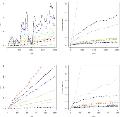
We perform a comparison on a data set of length T = _{20,000 simulated from the}

autoregres-sive model (20) with parameters θ∗ = _{(φ, σ, τ)}⊤ = _(0.8,0.5,1)⊤_{. Our method and the Poyiadjis}

O(N) have the same computational cost and are implemented with N = _{50,000. The Poyiadjis}

O(N2_{) algorithm, which has a quadratic computational cost, is implemented with N = 500. The}

comparisons were run on a Dell Latitude laptop with a 1.6GHz processor, where each iteration of

the_O(N) algorithms takes approximately 1 minute for N = _{50,000. TheO(N}2_{) takes 5.1 minutes}

for N 500. This corresponds to a CPU cost that is approximately 5 times greater than the_O(N)

methods.

The results given in Figure 1 show that for all but the Poyiadjis _O(N) algorithm the standard

deviation of the score estimate is increasing at a rate of T−1/2_{, giving a variance that is increasing}

approximately linearly with time. For the Poyiadjis_O(N), the variance is increasing quadratically

(standard deviation is increasing linearly) in line with the established theoretical results. As for the

O(N2) algorithm, the variance increases only linearly, as expected, but at an increased computa-tional cost compared to the_O(N) algorithms. The variance could be further reduced by increasing

the number of particles, but this will lead to a further increase in the computational cost. While

the variance of the_O(N2_{) is only linearly increasing, it is worth noting that it is larger than what is}

given by our algorithm for all values ofλ.

For estimating the score, the fixed-lag smoother performs well in terms of both bias and

vari-ance, and we note that, while not shown in Figure 1, varying the lag about log(T ) does not

dramat-ically change the outcome, but L= _{10 seems to give the best result. However, while the fixed-lag}

smoother appears to work well when estimating the score, it struggles to accurately estimate the

observed information, with a large bias for a range of lags (1 _≤ L _≤ 100). This is because the

fixed-lag approach reduces the variability in the estimates of _∇log p(x1:t,y1:t|θ) associated with

each particle, which means that it under-estimates the first term in Louis’s identity (9). Whilst our

approach also reduces the variability in the estimates of _∇log p(x1:t,y1:t|θ) associated with each

particle, we are able to correct for this within the Rao-Blackwellisation scheme (see Section 4.2

for details). This drawback is further explored in Section 7.1.

For our algorithm, we notice that the bias and variance of both the score estimate, and observed

information matrix, vary according toλ. Reducingλhas the eff_{ect of increasing the bias, but at}

the same time, reducing the Monte Carlo variance of the estimates. The figures show that if we

wish to minimise both bias and variance, then setting λ _≈ 0.95 will produce an estimate for the

score and observed information which exhibit only linearly increasing variance, with minimal bias

introduced as a result. In fact, the results suggest that setting 0.9 _≤ λ _≤ 0.99 will produce the

best overall results. However, ultimately interest lies in estimating the model parameters, and in

Section 7 we will see that our algorithm produces reliable estimates of the model parameters for

all values ofλ.

7

Parameter estimation

Our_O(N) algorithm, as described in Section 4, can be used to estimate the score vector and

ob-served information matrix. These estimates can then be used within the steepest ascent algorithm

(7) to obtain the MLE forθ.

The steepest ascent algorithm (7) performs offl_{ine maximum likelihood estimation using batches}

of data y1:T, which can be useful when dealing with small data sets. Alternatively, we could

im-plement recursive parameter estimation, where estimates of the parametersθt are updated as new

observations are made available. Ideally this would be achieved by using the gradient of the

pre-dictive log-likelihood,

θt = θt−1+γt∇log p(yt|y1:t−1, θt), (21)

where,

∇log p(yt|y1:t−1, θt)=∇log p(y1:t|θt)− ∇log p(y1:t−1|θt−1).

However, getting Monte Carlo estimates of _∇log p(yt|y1:t−1, θt) is difficult due to using different

values of θ at each iteration of the sequential Monte Carlo algorithm. Thus, following LeGland

and Mevel (1997) and Poyiadjis et al. (2011), we make a further approximation, and ignore the

fact thatθchanges with t. Instead we updateθt at each iteration using the following approximation

to this gradient:

∇log ˆp(yt|y1:t−1, θt)=St−St−1.

7.1

Autoregressive model

We compare the accuracy and effi_{ciency of estimating the parameters of the AR(1) model (20)}

using the various algorithms given in Section 6 in both an offl_{ine and online setting. Starting}

with the batch case (offl_{ine), we simulated 1,000 observations from the model with parameters}

θ∗ = _{(φ, σ, τ)}⊤ = _(0.9,0.7,1)⊤ _{and estimated the score vector and observed information}

ma-trix using our _O(N) algorithm, the fixed-lag smoother, and the _O(N) and _O(N2_{) algorithms of}

Poyiadjis. The estimates of the score vector and observed information matrix were used within

the Newton-Raphson algorithm (7) to estimate θ. The starting parameters for the algorithm are

θ0 = (φ, σ, τ)⊤ = (0.6,1,0.7)⊤. The AR(1) model is linear-Gaussian, and therefore allows for a

direct comparison against the Kalman filter, where the score and observed information matrix can

be calculated analytically.

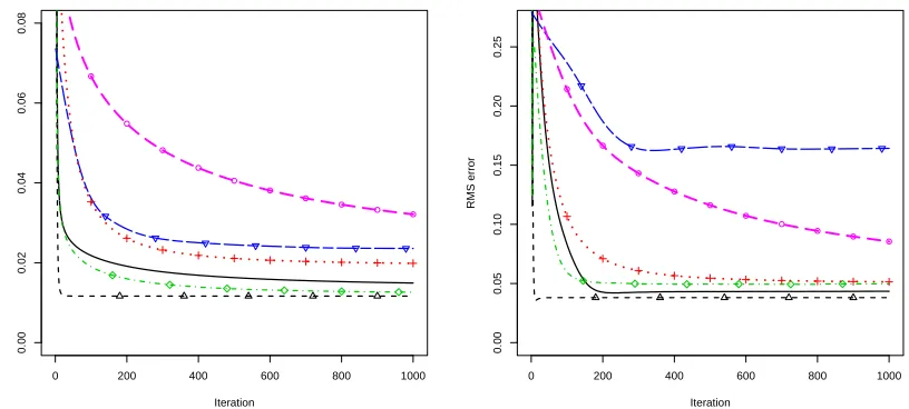
Figure 2 gives the RMS error of the parameters estimated using the Newton-Raphson algorithm

(7) averaged over 20 Monte Carlo simulations. Our algorithm, the fixed-lag smoother and the

O(N) algorithm of Poyiadjis were implemented with 50,000 particles and the _O(N2) algorithm was implemented with 1,000 particles. For our algorithm we set λ = _{0.95 and for the fixed-lag}

smoother L = _{7. In terms of computational cost, given the number of particles, our algorithm}

has more than a 10 fold computational time saving compared to the_O(N2_{) algorithm. The}

fixed-lag smoother was implemented with and without the observed information matrix applied in the

gradient ascent algorithm.

The RMS error of the _O(N2_{) algorithm given in Figure 2 is comparable to the error given by}

our_O(N) algorithm, however, it is important to remember that this is achieved with a significant

computational saving. Compared to the Poyiadjis _O(N) algorithm, our _O(N) algorithm and the

fixed-lag smoother (using only the score estimate) produce lower RMS error. Using a fixed-lag

smoother estimate of the observed information matrix in the Newton-Raphson algorithm leads

to higher RMS error than when only the score is used. The poor performance of the fixed-lag

approach was discussed in Section 6 and is attributed to the error in estimating the observed

infor-mation matrix.

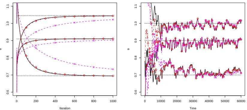
Illustrating the robustness ofλin our_O(N) algorithm, Figure 3 gives estimates forθusing the

offl_{ine (7) and online (21) gradient ascent algorithms for varying values ofλ(for the online case}

we simulated 60,000 observations). We see that there is little diff_{erence betweenλ} = _{0.99 and}

λ = _{0.95, but more importantly, forλ} = _{0.5 the parameters are converging to the MLEs, only at}

a slower rate. This was also the case for much lower choices ofλ(e.g. λ = _{0.1), which are not}

shown here, but for which the parameters converged to the MLE at an even slowly rate.

Using the recursive gradient ascent scheme (21) we can compare our method against the online

Bayesian particle learning algorithm (Carvalho et al., 2010). Particle learning uses MCMC moves

to sequentially update the parameters within an SMC algorithm. A prior distribution is selected for

each of the parameters which is updated at each time point via a set of low-dimensional suffi_cient

statistics (see the supplementary materials for implementation details).

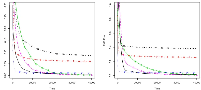
We generated 40,000 observations from the AR(1) model and considered three diff_{erent sets of}

true parameter values, chosen to represent diff_{erent degrees of dependence within the underlying}

state process: φ = _{0.9, 0.99 and 0.999. We setσ}2 _{= 1−φ}2 _{so that the marginal variance of the}

state is 1 and fixedτ = _{1. We maintain the same initial parametersθ0 for the gradient scheme as}

was used for the batch analysis.

Figure 4 shows the RMS error of our _O(N) algorithm applied to estimate the parameters θt,

against the particle learning filter over 100 data sets. The results show that the particle learning

filter produces a lower RMS error than our algorithm for the first few thousand observations, but

that it degenerates over very long time-series, particularly in the case of strong dependence (φ =

0.99 and 0.999). This is due to degeneracy in the suffi_{cient statistics that occurs as a result of}

their dependence on the complete latent process, and the fact that the Monte Carlo approximation

to p(x1:T|y1:T, θ) degrades as T increases (Andrieu et al., 2005). This degeneracy is particularly

pronounced for largeφ, as this corresponds to cases where the underlying MCMC moves used to

update the parameters mix poorly.

Over longer data sets, applying gradient ascent with our_O(N) algorithm, outperforms particle

learning. Asφapproaches 1, the long term state dependence is increased, as is the distance between

the true parameter values and the fixed starting values used to initiate the gradient scheme. Our

method appears to take longer to converge in this setting, but compared to particle learning, our

method appears to be more robust to the choice of φ, and for this reason, maximum likelihood

methods are preferred over particle learning when estimating parameters from long time series.

See Chopin et al. (2011) for a further discussion on the implementation challenges of particle

learning.

7.2

Nonlinear seasonal Poisson model

In this section we demonstrate our methodology on a nonlinear state space model, where we

es-timate the parameters from a real data set and show that these eses-timates are in agreement with

previous studies.

We consider a time series of monthly counts of poliomyelitis in the United States from January

1970 to December 1983. This time series was introduced by Zeger (1988) and has since been

analysed by Chan and Ledolter (1995), who used a Monte Carlo EM algorithm, and Davis and

Rodriguez-Yam (2005) and Langrock (2011) who both estimated the parameters using an

approx-imate likelihood approach. The proposed model accounts for the observed seasonality of polio

outbreaks and also contains a trend component which is the main interest in determining whether

or not there is a decreasing trend:

Yt|Xt = xt,zt ∼ Nt[0,xtexp(zt)], Xt|Xt−1= xt−1∼ N(φxt−1, σ2) (22)

log(zt)= μ1+μ2

t

1000 +μ3cos 2πt

12

!

+_μ4sin 2πt

12

!

+_μ5cos 2πt

12

!

+_μ6sin 2πt

12

!

,

where Nt[a,b] denotes the number of events in time interval (a,b].

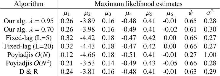
The model parametersθ=_{(μ1, μ2, μ3, μ4, μ5, μ6, φ, σ}2₎⊤_{are estimated using the gradient ascent}

algorithm, where the score vector is estimated using our proposed method (Alg. 2) withλ= _0.95

and 0.7. We compare our method against the fixed-lag smoother and the Poyiadjis_O(N) and_O(N2) algorithms. Each method was implemented with N = _{1,000 particles, except the PoyiadjisO(N}2₎

algorithm, which was implemented with N =_33≈ √_{1,000 . The fixed-lag smoother was run with}

lag L=_{5 and 20.}

Parameter estimates for the seasonal Poisson model are given in Table 1, where the batch

implementation of the gradient ascent algorithm was executed for 2,000 iterations. Given the

short data set (T=_{168), we do not consider recursive parameter estimation.}

We give the results from using our method with λ = _{0.95 and λ} = _{0.7, and note that almost}

identical parameter estimates were obtained forλ _∈ [0.5,0.99]. We can see that for our method,

the parameter estimates are consistent with the results presented by Davis and Rodriguez-Yam

(2005) and Langrock (2011). To understand the performance of the methods we re-ran each of

them 20 times to see the Monte Carlo variability in the parameter estimates. For our method, the

fixed-lag smoother and the _O(N2_{) method, we obtained almost identical estimates for each run.}

However the _O(N) method of Poyiadjis et al. showed increased variation in the estimates (for

example the range of the estimates forμ2 was [-4.76, -4.53]). The fixed-lag smoothers performed

equally well for L= _{5 and 20 with little di}ff_{erence between the two implementations. Most of the}

parameters are estimated well using the fixed-lag smoother, but the bias of the score estimates does

lead to poor estimation of μ1 andμ2. All of the algorithms, except the PoyiadjisO(N) andO(N2)

algorithms converged after approximately 500 iterations (figures available in the supplementary

material). This is due to the Monte Carlo variation in the score estimates which directly impacts

the parameter estimates. In the case of the _O(N2_{) algorithm, this variation could be reduced by}

increasing the number of particles, but at a significantly increased computational cost compared to

our method.

8

Discussion

In this paper we have presented a novel sequential Monte Carlo method for estimating the score

vector and observed information matrix for nonlinear, non-Gaussian state space models. Previous

approaches have produced estimates with quadratically increasing variance at a computational

cost that is linear in the number of particles, or achieved linearly increasing variance at a quadratic

computational cost.

The algorithm we have developed combines techniques from kernel density estimation and

Rao-Blackwellisation to yield estimates of both the score vector and the observed information

matrix which display only linearly increasing variance, which is achieved at a linear

computa-tional cost. Importantly, we have shown that this approximate score vector, at the true parameter

value, has expectation zero when taken with respect to the data. Thus, the resulting gradient

as-cent scheme uses Monte Carlo methods to approximately find the solution to a set of unbiased

estimating equations.

The estimates of the score and observed information given by our _O(N) algorithm can be

ap-plied to the gradient ascent and Newton-Raphson algorithms to obtain maximum likelihood

esti-mates of the model parameters. This can be achieved either offl_{ine or online, where the parameters}

are estimated from a batch of observations, or recursively from observations received sequentially.

Furthermore, we have shown that in terms of parameter estimation, our algorithm is relatively

in-sensitive the the choice of λ. However we do note that setting 0.90 < λ < 0.99 produces low

variance estimates of the score with minimal bias, which also results in faster parameter

conver-gence.

For a significant reduction in computational time we can achieve improved parameter

estima-tion over competing methods in terms of minimising root mean squared error. We also compared

our algorithm to the particle learning filter for online estimation. The particle learning filter

per-forms well initially but degenerates over time, whereas our algorithm is more accurate over longer

time series. Our method also appears to be robust to the choice of model parameters compared

to the particle learning filter which struggles to estimate the parameters when the states are highly

dependent.

Supplementary Materials

Appendices: Proofs for Lemma 1 and Theorem 1. Also, a derivation of the particle learning

updates and a plot for the nonseasonal Poisson model example. (pdf)

R code: R code for the examples in Section 7. (Rcode.zip, zip file)

References

Andrieu, C., Doucet, A., and Tadic, V. B. (2005). On-line parameter estimation in general

state-space models. In IEEE Conference on Decision and Control, pages 332–337.

Capp´e, O., Godsill, S., and Moulines, E. (2007). An Overview of Existing Methods and Recent

Advances in Sequential Monte Carlo. Proceedings of the IEEE, 95(5):899–924.

Capp´e, O., Moulines, E., and Ryden, T. (2005). Inference in Hidden Markov Models. Springer

Series in Statistics. Springer.

Carvalho, C. M., Johannes, M., Lopes, H., and Polson, N. G. (2010). Particle Learning and

Smoothing. Statistical Science, 25(1):88–106.

Chan, K. and Ledolter, J. (1995). Monte Carlo EM estimation for time series models involving

counts. Journal of the American Statistical Association, 90(429):242–252.

Chopin, N. (2004). Central limit theorem for sequential Monte Carlo methods and its application

to Bayesian inference. The Annals of Statistics, 32(6):2385–2411.

Chopin, N., Iacobucci, A., Marin, J., Mengersen, K., Robert, C., Ryder, R., and Sh afer, C. (2011).

On particle learning. In Bernardo, J., Bayarri, M., Berger, J., Dawid, A., D.Heckerman, Smith,

A., and West, M., editors, Bayesian Statistics 9, pages 317–360. Oxford University Press.

Crisan, D. and Doucet, A. (2002). A survey of convergence results on particle filtering methods

for practitioners. IEEE Transactions on Signal Processing, 50(3):736–746.

Crowder, M. (1986). On consistency and inconsistency of estimating equations. Econometric

Theory, 2(3):305–330.

Dahlin, J., Lindsten, F., and Sch¨on, T. B. (2014). Second-order Particle MCMC for Bayesian

Parameter Inference. In Proceedings of the 19th World Congress of the International Federation

of Automatic Control (IFAC).

Davis, R. and Rodriguez-Yam, G. (2005). Estimation for state-space models based on a likelihood

approximation. Statistica Sinica, 15:381–406.

Del Moral, P., Doucet, A., and Singh, S. S. (2010). A backward particle interpretation of

Feynman-Kac formulae. ESAIM: Mathematical Modelling and Numerical Analysis, 44(5):947–975.

Douc, R., Garivier, A., Moulines, E., and Olsson, J. (2011). Sequential monte carlo smoothing

for general state space hidden markov models. The Annals of Applied Probability, 21(6):2109–

2145.

Doucet, A., Godsill, S., and Andrieu, C. (2000). On sequential Monte Carlo sampling methods for

Bayesian filtering. Statistics and computing, 10(3):197–208.

Durbin, J. and Koopman, S. (2001). Time Series Analysis by State Space Methods. Oxford

Statis-tical Science Series. Oxford University Press.

Fearnhead, P. (2007). Computational methods for complex stochastic systems: a review of some

alternatives to MCMC. Statistics and Computing, 18(2):151–171.

H¨urzeler, M. and K¨unsch, H. R. (2001). Approximating and maximising the likelihood for a

general state-space model. In Doucet, A., de Freitas, N., and Gordon, N., editors, Sequential

Monte Carlo Methods in Practice, pages 197–223. Springer-Verlag, New York.

Kalman, R. E. (1960). A New Approach to Linear Filtering and Prediction Problems. Transactions

of the ASME, Journal of Basic Engineering, 82(Series D):35–45.

Kitagawa, G. and Sato, S. (2001). Monte carlo smoothing and self-organising state-space model.

In Doucet, A., de Freitas, N., and Gordon, N., editors, Sequential Monte Carlo Methods in

Practice, pages 178–195. Springer-Verlag, New York.

Langrock, R. (2011). Some applications of nonlinear and non-Gaussian statespace modelling by

means of hidden Markov models. Journal of Applied Statistics, 38(12):2955–2970.

LeGland, F. and Mevel, L. (1997). Recursive estimation in hidden Markov models. In 36th IEEE

Conference on Decision and Control, pages 3468–3473, San Diego, CA. Institute of Electronics

and Electrical Engineering.

Liu, J. and West, M. (2001). Combined parameter and state estimation in simulation-based

filter-ing. In Doucet, A., de Freitas, N., and Gordon, N., editors, Sequential Monte Carlo Methods in

Practice, pages 197–223. Springer-Verlag, New York.

Louis, T. (1982). Finding the observed information matrix when using the EM algorithm. Journal

of the Royal Statistical Society. Series B, 44(2):226–233.

Olsson, J., Capp´e, O., Douc, R., and Moulines, E. (2008). Sequential Monte Carlo smoothing with

application to parameter estimation in nonlinear state space models. Bernoulli, 14(1):155–179.

Olsson, J. and Westerborn, J. (2014). Effi_{cient particle-based online smoothing in general hidden}

Markov models: the PaRIS algorithm. arXiv preprint arXiv:1412.7550.

Pitt, M. K. and Shephard, N. (1999). Filtering via Simulation: Auxiliary Particle Filters. Journal

of the American Statistical Association, 94(446):590–599.

Poyiadjis, G., Doucet, A., and Singh, S. S. (2011). Particle approximations of the score and

observed information matrix in state space models with application to parameter estimation.

Biometrika, 98(1):65–80.

Westerborn, J. and Olsson, J. (2014). Effi_{cient particle based online smoothing in general}

hid-den markov models. In International Conference on Acoustics, Speech and Signal Processing

(ICASSP).

Zeger, S. (1988). A regression model for time series of counts. Biometrika, 75(4):621–629.

0 5000 10000 15000 20000

0

5

10

15

Time

Bias

0 5000 10000 15000 20000

0

2

4

6

8

10

Time

Standard De

viation

0 200 400 600 800 1000

0

200

400

600

800

Time

Bias

0 200 400 600 800 1000

0

10

20

30

40

50

60

Time

Standard De

viation

Figure 1: Absolute bias (left column) and standard deviation (right column) of score estimates for

τ(top row) and observed information matrix for theφcomponent (bottom row) from the autore-gressive model using our_O(N) algorithm withλ= _{0.99 ( ∗ ∗ ),λ} = _{0.95 ( ),λ} = _0.9

(−∙ ×−∙ ×−),λ=0.8 ( ^ ^ ),λ=0.7 ( △ △ ), Fixed-lag smoother L =10 (∙▽∙ ∙▽∙ ∙▽∙

), and the Poyiadjis_O(N) algorithm (· · · · ··) andO(N2) with N =500 (−∙ ⊗−∙ ⊗−).

0 200 400 600 800 1000

0.00

0.02

0.04

0.06

0.08

Iteration

RMS error

0 200 400 600 800 1000

0.00

0.05

0.10

0.15

0.20

0.25

Iteration

RMS error

Figure 2: Root mean squared error of parameter estimatesφ(left panel) and σ(right panel) aver-aged over 20 Monte Carlo simulations from our _O(N) algorithm withλ = _{0.95 ( ), Poyiadjis}

O(N) ( _{▽ ▽} ), Poyiadjis_O(N2) (−∙^−∙−^), Fixed-lag smoother ( ◦ ◦ ), Fixed-lag

smoother (· ·+· ·+·) with score only and the Kalman filter estimate ( △ △ ).

0 200 400 600 800 1000

0.6

0.7

0.8

0.9

1.0

1.1

Iteration

θ

0 10000 20000 30000 40000 50000 60000

0.6

0.7

0.8

0.9

1.0

1.1

Time

θ

Figure 3: Batch (left panel) and recursive (right panel) parameter estimation forλ = _{0.99 ( ),} λ=_{0.95 (−∙}^_−∙−^_{) andλ}= _{0.5 ( × × ).}

0 10000 20000 30000 40000

0.00

0.05

0.10

0.15

0.20

0.25

0.30

Time

RMS Error

0 10000 20000 30000 40000

0.0

0.2

0.4

0.6

0.8

1.0

Time

RMS Error

Figure 4: Root mean squared error of parameter estimates φ (left panel) and σ(right panel) av-eraged over 100 Monte Carlo simulations from our algorithm withλ = _{0.95 andφ} = _{0.9 ( ),} φ=_{0.99 ( △ △ ),φ}= _{0.999 (} ^ ^ _{) and the particle learning algorithm withφ}= _0.9

(_{∙▽∙ ∙▽∙ ∙∙}),φ=_{0.99 (−◦ ∙−◦ ∙−),φ}= _{0.999 (··×··×··).}

Table 1: Results of batch parameter estimation for competing models using the gradient ascent algorithm (7) initialised at θ0 = (0.4,−3,0.3,−0.3,0.65,−0.2,0.4,0.4). Results given by Davis

and Rodriguez-Yam (2005) are quoted as D&R.

Algorithm Maximum likelihood estimates

μ1 μ2 μ3 μ4 μ5 μ6 φ σ2

Our alg.λ= _{0.95 0.26 -3.89 0.16 -0.48 0.41 -0.01 0.65 0.28}

Our alg.λ= _{0.70 0.26 -3.98 0.16 -0.49 0.41 -0.02 0.61 0.30}

Fixed-lag (L=_{5) 0.32 -4.42 0.18 -0.47 0.42 0.00 0.66 0.27}

Fixed-lag (L=_{20) 0.32 -4.43 0.18 -0.47 0.42 0.00 0.66 0.27}

Poyiadjis_O(N) 0.12 -4.66 0.18 -0.51 0.41 -0.01 0.27 1.00 Poyiadjis_O(N2_{) 0.21 -3.53 0.14 -0.49 0.43 -0.05 0.66 0.28}

D & R 0.24 -3.81 0.16 -0.48 0.41 -0.01 0.63 0.29