The rate of convergence for approximate Bayesian computation

This is a repository copy of The rate of convergence for approximate Bayesian

computation.

White Rose Research Online URL for this paper:

http://eprints.whiterose.ac.uk/84057/

Version: Accepted Version

Article:

Barber, S, Voss, J and Webster, M (2015) The rate of convergence for approximate

Bayesian computation. Electronic Journal of Statistics, 9 (1). pp. 80-105. ISSN 1935-7524

https://doi.org/10.1214/15-EJS988

eprints@whiterose.ac.uk https://eprints.whiterose.ac.uk/ Reuse

Unless indicated otherwise, fulltext items are protected by copyright with all rights reserved. The copyright exception in section 29 of the Copyright, Designs and Patents Act 1988 allows the making of a single copy solely for the purpose of non-commercial research or private study within the limits of fair dealing. The publisher or other rights-holder may allow further reproduction and re-use of this version - refer to the White Rose Research Online record for this item. Where records identify the publisher as the copyright holder, users can verify any specific terms of use on the publisher’s website.

Takedown

If you consider content in White Rose Research Online to be in breach of UK law, please notify us by

ISSN: 1935-7524 arXiv:arXiv:1311.2038

The Rate of Convergence for

Approximate Bayesian Computation

Stuart Barber and Jochen Voss and Mark Webster

School of Mathematics University of Leeds Leeds LS2 9JT, UK e-mail:s.barber@leeds.ac.uk

e-mail:j.voss@leeds.ac.uk

e-mail:mm08mgw@leeds.ac.uk

Abstract: Approximate Bayesian Computation (ABC) is a popular compu-tational method for likelihood-free Bayesian inference. The term “likelihood-free” refers to problems where the likelihood is intractable to compute or estimate directly, but where it is possible to generate simulated dataX relatively easily given a candidate set of parametersθsimulated from a prior distribution. Parameters which generate simulated data within some toleranceδof the observed datax∗_{are regarded as plausible, and a collection} of suchθis used to estimate the posterior distributionθ|X=x∗_{. Suitable} choice ofδis vital for ABC methods to return good approximations toθin reasonable computational time.

While ABC methods are widely used in practice, particularly in pop-ulation genetics, rigorous study of the mathematical properties of ABC estimators lags behind practical developments of the method. We prove that ABC estimates converge to the exact solution under very weak assump-tions and, under slightly stronger assumpassump-tions, quantify the rate of this convergence. In particular, we show that the bias of the ABC estimate is asymptotically proportional toδ2_{asδ↓0. At the same time, the} compu-tational cost for generating one ABC sample increases likeδ−q _whereqis

the dimension of the observations. Rates of convergence are obtained by optimally balancing the mean squared error against the computational cost. Our results can be used to guide the choice of the tolerance parameterδ.

MSC 2010 subject classifications:Primary 62F12, 65C05; secondary 62F15.

Keywords and phrases:Approximate Bayesian Computation, likelihood-free inference, Monte Carlo methods, convergence of estimators, rate of convergence.

1. Introduction

Approximate Bayesian Computation (ABC) is a popular method for likelihood-free Bayesian inference. ABC methods were originally introduced in popula-tion genetics, but are now widely used in applicapopula-tions as diverse as epidemiol-ogy (Tanaka et al.,2006;Blum and Tran,2010;Walker et al.,2010), materials science (Bortot et al.,2007), parasitology (Drovandi and Pettitt,2011), genetic evolution (Thornton and Andolfatto,2006;Fagundes et al.,2007;Ratmann et al.,

2009;Wegmann and Excoffier,2010;Beaumont,2010;Wilkinson et al.,2011),

population migration (Guillemaud et al., 2010) and conservation studies (Lopes and Boessenkool,2010).

One of the earliest articles about the ABC approach, covering applications in population genetics, isTavar´e et al.(1997). Newer developments and extensions of the method include placing ABC in an MCMC context (Marjoram et al.,

2003), sequential ABC (Sisson et al., 2007), enhancing ABC with nonlinear regression models (Blum and Fran¸cois,2010), agent-based modelling (Sottoriva and Tavar´e,2010), and a Gibbs sampling ABC approach (Wilkinson et al.,2011). A survey of recent developments is given byMarin et al.(2012).

ABC methods allow for inference in a Bayesian setting where the parameter

θ ∈ Rp _{of a statistical model is assumed to be random with a given prior}

distributionfθ, we have observed dataX ∈Rd from a given distributionfX|θ

depending onθ and we want to use these data to draw inference aboutθ. In the areas where ABC methods are used, the likelihoodfX|θis typically not available

in an explicit form. The term “likelihood-free” is used to indicate that ABC methods do not make use of the likelihoodfX|θ, but only work with samples

from the joint distribution of θ andX. In the context of ABC methods, the data are usually summarised using a statisticS:Rd_→Rq_{, and analysis is then}

based onS(X) instead ofX. The choice ofS affects the accuracy of the ABC estimates: the estimates can only be expected to converge to the true posterior ifS is a sufficient statistic, otherwise additional error is introduced.

The basic idea of ABC methods is to replace samples from the exact posterior distribution θ_|X =x∗ _orθ

|S(X) =s∗ _{with samples from an approximating} distribution likeθ_|S(X)_≈s∗_{. There are many variants of the basic ABC method} available, including different implementations of the conditionS(X)_≈s∗_{. All} variants use a tolerance parameterδwhich controls the trade-off between fast generation of samples (large values ofδ) and accuracy of samples (small values ofδ). The easiest approach to implement the conditionS(X)≈s∗_{, considered in} this paper, is to usekS(X)−s∗_{k ≤δwherek · k is some norm onR}q_{. Different}

approaches to choosing the statistic S are used; a semi-automatic approach is described in Fearnhead and Prangle (2012). In many cases considerable improvements can be achieved by choosing the norm for comparison ofS(X) to

s∗ _{in a problem-specific way.}

Despite the popularity of ABC methods, theoretical analysis is still in its infancy. The aim of this article is to provide a foundation for such analysis by providing rigorous results about the convergence properties of the ABC method. Here, we restrict discussion to the most basic variant, to set a baseline to which different ABC variants can be compared. We consider Monte Carlo estimates of posterior expectations, using the ABC samples for the estimate. Proposition3.1

shows that such ABC estimates converge to the true value under very weak conditions; once this is established we investigate the rate of convergence in theorem3.3. Similar results, but in the context of estimating posterior densities rather than posterior expectations can be found inBlum (2010) andBiau et al.

(2013). Further studies will be required to establish analogous results for more complex ABC variants,e.g.SMC or MCMC based algorithms.

the practical application of ABC methods, but not many results are available in the literature. A numerical study of the trade-off between accuracy and computational cost, in the context of sequential ABC methods, can be found inSilk et al. (2013).Wilkinson(2013) establishes that an ABC method which accepts or rejects proposals with a probability based on the difference between the observed and proposed data converges to the correct solution under assumptions on model or measurement error.

The error of an ABC estimate is affected both by the bias of the ABC samples, controlled by the tolerance parameterδ, and by Monte Carlo error, controlled by the numbernof accepted ABC samples. One of the key ingredients in our analysis is the result, shown in lemma 3.6, that for ABC estimates the bias satisfies

bias∼δ2.

Similarly, in lemma3.7we show that the computational cost,i.e.the CPU time required to compute the ABC estimate, satisfies

cost_∼nδ−q,

whereq is the dimension of the observations∗_.

It is well-known that for Monte Carlo methods the error decays, as a function of computational cost, proportional to cost−1/2_{, where the exponent −1/2 is} independent of dimension (seee.g. Voss,2014, section 3.2.2). In contrast, the main result of this article, theorem3.3, shows that, under optimal choice ofδ, the basic ABC method satisfies

error_∼cost−2/(q+4).

Corollary4.2shows that this result holds whether we fix the number of accepted samples (controlling the precision of our estimates but allowing the computational cost to be random) or fix the number of proposals (allowing the number of accepted samples to be random). The former is aesthetically more satisfying, but in practice most users have a fixed computational budget and hence must fix the number of proposals. In either case, the rate of decay for the error gets worse as the dimensionq increases and even in the one-dimensional case the exponent

−2/(1 + 4) =₋2/5 is worse than the exponent₋1/2 for Monte Carlo methods.

Fearnhead and Prangle (2012) obtain the same exponent ₋2/(q+ 4) for the specific summary statisticS(X) =E_{(θ|X). For the problem of estimating the}

posterior density,Blum(2010) reports the slightly worse exponent₋2/(q+ 5). The difference between Blum’s results and ours is due to the fact that for kernel density estimation an additional bandwidth parameter must be considered.

2. Approximate Bayesian Computation

This section gives a short introduction to the basic ABC algorithm. A more complete description is, for example, given inVoss(2014, section 5.1). We describe the algorithm in the context of the following Bayesian inference problem:

• A parameter vectorθ_∈Rp_{is assumed to be random. Before observing any}

data, our belief about its value is summarised by the prior distributionfθ.

The value ofθ is unknown to us and our aim is to make inference aboutθ.

• The available dataX_∈Rd _{are assumed to be a sample from a distribution}

fX|θ, depending on the parameterθ. Inference aboutθis based on a single

observed samplex∗ _{from this distribution; repeated observations can be} assembled into a single vector if needed.

• In the context of ABC, the data are often summarised using a statistic

S:Rd_→Rq_{. SinceX is random,S =S(X) is random with a distribution}

fS|θ depending onθ. If a summary statistic is used, inference is based on

the values∗_=S(x∗_{) instead of on the full samplex}∗_.

Our aim is to explore the posterior distribution ofθ,i.e.the conditional distri-bution ofθgivenX =x∗_{, using Monte Carlo methods. More specifically, we aim} to estimate the posterior expectations

y=E h(θ) X =x∗

(1)

for given test functionsh:Rp_→R_{. Expectations of this form allow us to study}

many relevant properties of the posterior distribution, including the posterior mean when h(θ) =θi with i= 1, . . . , pand posterior second moments when

h(θ) =θiθj with i, j = 1, . . . , p. If h(θ) = 1A(θ) for a given set A ⊆Rp, the

expectationE h(θ)X =x∗

equals the posterior probability of hittingA; for example, the CDF can be approximated by choosingA= (_−∞, a] fora_∈R_.

The basic ABC method for generating approximate samples from the posterior distribution is given in the following algorithm.

Algorithm 2.1. For a given observations∗ _∈Rq _{and given tolerance δ >0,}

ABC samplesapproximating the distribution θ|S = s∗ _{are random samples}

θ(jδ)∈Rpcomputed by the following algorithm: 1: letj←0

2: whilej < ndo

3: sampleθwith densityfθ(·) 4: sampleX with densityfX|θ(· |θ) 5: if _kS(X)₋s∗

kA≤δthen 6: letj←j+ 1

7: letθ(_jδ)←θ 8: end if 9: end while

The normk · kA used in the acceptance criterion is defined byksk2A=s⊤A−1s

case of the Euclidean distancek · k=k · kI forA=I. In practical applications,

the matrixAis often chosen in a problem-specific way.

Using the output of the algorithm, an estimate for the posterior expectation (1) can be obtained as

Y(δ)

n =

1

n

n X

j=1

h(θ(_jδ)) (2)

whereθ₁(δ), . . . , θ(nδ)are computed by algorithm2.1. Since the output of the ABC

algorithm approximates the posterior distribution, the Monte Carlo estimateYn(δ)

can be used as an approximation to the posterior expectation.

The ABC samples are only approximately distributed according to the pos-terior distribution, and thus the estimateYn(δ) will not exactly converge to the

true value y asn _{→ ∞}. The quality of the approximation can be improved by decreasing the tolerance parameterδ, but this leads at the same time to a lower acceptance probability in algorithm2.1 and thus, ultimately, to higher computational cost for obtaining the estimateYn(δ). Hence, a trade-off must be

made between accuracy of the results and speed of computation.

Since the algorithm is not usingx∗ _{directly, but usess}∗_=S(x∗_{) instead, we} requireS to be a sufficient statistic, so that we have

y=E h(θ) X =x∗

=E h(θ) S =s∗

.

IfS is not sufficient, an additional error will be introduced.

Forapplicationof the ABC method, knowledge of the distributions ofθ, X

andS=S(X) is not required; instead we assume that we can simulate large numbers of samples of these random variables. In contrast, in ouranalysis we will assume that the joint distribution ofθandS has a densityfS,θ and we will

need to consider properties of this density in some detail.

To conclude this section, we remark that there are two different approaches to choosing the sample size used to compute the ABC estimate Yn(δ). If we

denote the number of proposals required to generatenoutput samples byN≥n, then one approach is to choose the number N of proposals as fixed; in this case the number n ≤ N of accepted proposals is random. Alternatively, for givenn, the loop in the ABC algorithm could be executed untilnsamples are accepted, resulting in randomN and fixedn. In order to avoid complications with the definition of Yn(δ) forn= 0, we follow the second approach here and

defer discussion of the case of fixedN until section4.

3. Results

This section presents the main results of the paper, in proposition 3.1 and theorem3.3, followed by proofs of these results.

Throughout, we assume that the joint distribution ofθandS has a density

fS,θ, and we consider the marginal densities ofS andθgiven by

fS(s) = Z

Rp

for alls∈Rq _and

fθ(t) = Z

Rq

fS,θ(s, t)ds

for allt_∈Rp_{, respectively. We also consider the conditional density ofθ given}

S=s, defined by

fθ|S(t|s) =

(_fS,θ(s,t)

fS(s) , iffS(s)>0, and

0 otherwise.

Our aim is to study the convergence of the estimateYn(δ) to y as n→ ∞.

The fact that ABC estimates converge to the correct value as δ_↓0 is widely accepted and easily shown empirically. This result is made precise in the following proposition, showing that the convergence holds under very weak conditions.

Proposition 3.1. Let h: Rp _→ R _{be such that} E _|h(θ)|

< _∞. Then, for

fS-almost alls∗∈Rq, the ABC estimateYn(δ) given by (2)satisfies

1. lim

n→∞Y (δ)

n =E Yn(δ)

almost surely for allδ >0; and 2. lim

δ↓0

E _Yn(δ)

=E h(θ) S =s∗

for all n_∈N_.

We note that the assumptions required in our version of this result are very modest. Since our aim is to estimate the posterior expectation of h(θ), the assumption that the prior expectationE _|h(θ)|

exists is reasonable. Similarly, the phrase “forfS-almost alls∗∈Rq” in the proposition indicates that the result

holds for alls∗ _{in a setA}

⊆Rq _{withP S(X)∈A}

= 1. Since in practice the values∗ _{will be an observed sample ofS(X), this condition forms no restriction} to the applicability of the result. The proposition could be further improved by removing the assumption that the distributions ofθandS(X) have densities. While a proof of this stronger result could be given following similar lines to the proof given below, here we prefer to keep the setup consistent with what is required for the result in theorem3.3.

Our second result, theorem3.3, quantifies the speed of convergence ofYn(δ)

toy. We consider the mean squared error MSE(Yn(δ)) =E (Yn(δ)−y)2

= Var(Yn(δ)) + bias(Yn(δ))2,

and relate this to the computational cost of computing the estimateYn(δ). For

the computational cost, rather than using a sophisticated model of computation, we restrict ourselves to the na¨ıve approach of assuming that the time required to obtain the estimateYn(δ)in algorithm2.1, denoted cost(Yn(δ)), is proportional

toa+bN, whereaandb are constants andN is the number of iterations the while-loop in the algorithm has to perform until the condition j = n is met (i.e.the number of proposals required to generatensamples). To describe the

Notation. For sequences (an)n∈N and (bn)n∈N of positive real numbers we writean ∼bn to indicate that the limit c= limn→∞an/bn exists and satisfies

0<_|c_|<_∞.

In our results it will be convenient to use the following technical notation.

Definition 3.2. Forh: Rp_→R_with E _{|h(θ)|<∞we defineϕh:}Rq _→R_to

be

ϕh(s) = Z

Rp

h(t)fS,θ(s, t)dt

for alls_∈Rq _andϕ(δ)

h :Rq →Rto be

ϕ(_hδ)(s∗) = 1 B(s∗, δ)

Z

B(s∗_,δ)

ϕh(s)ds, (3)

for alls∗

∈Rq_{, where}B(s∗, δ)

denotes the volume of the ballB(s∗, δ).

Using the definition for h _≡ 1 we get ϕ1 ≡ fS and for general h we get

ϕh(s) = fS(s)E h(θ) S = s

. Our result about the speed of convergence requires the density ofS(X) to have continuous third partial derivatives. More specifically, we will use the following technical assumptions onS.

Assumption A. The densityfS and the function ϕh are three times

continu-ously differentiable in a neighbourhood ofs∗_∈Rq_. Theorem 3.3. Leth: Rp_→R_{be such that}E _h(θ)2

<_∞and letSbe sufficient and satisfy assumption A. AssumeVar h(θ)

S=s∗

>0 and

C(s∗) = ∆ϕh(s

∗_)−y·∆ϕ 1(s∗) 2(q+ 2)ϕ1(s∗) 6

= 0 (4)

where∆denotes the Laplace operator. Then, forfS-almost alls∗, the following

statements hold:

1. Let (δn)n∈Nbe a sequence with δ_n∼n−1/4. Then the mean squared error

satisfies

MSE(Y(δn)

n )∼E cost(Yn(δn))

−4/(q+4)

asn→ ∞.

2. The exponent −4/(q+ 4) given in the preceding statement is optimal: for any sequence(δn)n∈N withδn↓0 asn→ ∞we have

lim inf

n→∞

MSE(Y(δn)

n )

E _cost(Y(δn)

n )−4/(q+4)

>0.

proportional ton. Thus, for Monte Carlo estimates we have RMSE∼cost−1/2. The corresponding exponent from theorem3.3, obtained by taking square roots, is ₋2/(q+ 4), showing slower convergence for ABC estimates. This reduced efficiency is a consequence of the additional error introduced by the bias in the ABC estimates.

The statement of the theorem implies that, as computational effort is increased,

δshould be decreased proportional ton−1/4_{. For this case, the error decreases} proportionally to the cost with exponentr=₋4/(q+ 4). The second part of the theorem shows that no choice ofδcan lead to a better (i.e.more negative) exponent. If the tolerancesδnare decreased in a way which leads to an exponent

˜

r > r, in the limit for large values ofnsuch a schedule will always be inferior to the choiceδn =cn−1/4, for any constantc >0. It is important to note that this

result only applies to the limitn→ ∞.

The result of theorem3.3describes the situation where, for a fixed problem, the toleranceδis decreased. Caution is advisable when comparing ABC estimates for different q. Since the constant implied in the _∼-notation depends on the choice of problem, and thus onq, the dependence of the error on qfor fixedδis not in the scope of theorem3.3. Indeed,Blum(2010) suggests that in practice ABC methods can be successfully applied for larger values ofq, despite results like theorem3.3.

Before we turn our attention to proving the results stated above, we first remark that, without loss of generality, we can assume that the acceptance criterion in the algorithm uses Euclidean distance _{k · k} instead of_{k · k}A. This

can be achieved by considering the modified statistic ˜S(x) =A−1/2_{S(x) and} ˜

s∗_{= ˜S(x}∗_{) =A}−1/2_s∗_{, whereA}−1/2 _{is the positive definite symmetric square} root ofA−1_{. Since}

S(X)−s∗

2

A= S(X)−s

∗⊤

A−1 _S(X)

−s∗

=A−1/2 S(X)₋s∗⊤

A−1/2 S(X)₋s∗

=S˜(X)−˜s∗

2

,

the ABC algorithm usingS and_{k · k}Ahas identical output to the ABC algorithm

using ˜S and the Euclidean norm. Finally, a simple change of variables shows that the assumptions of proposition3.1and theorem3.3are satisfied forS and

k · kA if and only they are satisfied for ˜S andk · k. Thus, for the proofs we will

assume that Euclidean distance is used in the algorithm.

The rest of this section contains the proofs of proposition3.1and theorem3.3. We start by showing that both the exact valuey from (1) and the mean of the estimatorYn(δ)from (2) can be expressed in the notation of definition3.2. Lemma 3.4. Let h:Rp_→R_{be such that}E _|h(θ)|

<_∞. Then

E _h(θ)S=s∗

= ϕh(s ∗₎

and

E _Yn(δ)₌E _h(θ1(δ)₎₌ϕ

(δ)

h (s∗)

ϕ(1δ)(s∗) forfS-almost all s∗∈Rq.

Proof. From the assumption E _|h(θ)|

<∞we can conclude

Z

Rq

Z

Rp

h(t)

fS,θ(s, t)dt ds= Z

Rp

h(t)

Z

Rq

fS,θ(s, t)ds dt

=

Z

Rp

h(t)

fθ(t)dt=E |h(θ)|<∞,

and thus we know thatR

Rp

h(t)

fS,θ(s, t)dt <∞for almost alls∈Rq.

Conse-quently, the conditional distribution E _h(θ)S =s∗

exists forfS-almost all

s∗

∈Rq_{. Using Bayes’ rule we get}

E _h(θ)S=s∗

=

Z

Rp

h(t)fθ|S(t|s∗)dt

=

Z

Rp

h(t)fS,θ(s ∗_{, t)}

fS(s∗)

dt= ϕh(s ∗₎

ϕ1(s∗)

.

On the other hand, the samplesθ(_jδ)are distributed according to the conditional distribution ofθ givenS ∈B(s∗, δ). Thus, the density of the samplesθ(jδ)can

be written as

f_θ(δ)

j

(t) = 1

Z

1

B(s∗, δ) Z

B(s∗,δ)

fS,θ(s, t)ds,

where the normalising constantZ satisfies

Z= 1 B(s∗, δ)

Z

B(s∗_,δ)

fS(s)ds=

1

B(s∗, δ)

Z

B(s∗_,δ)

ϕ1(s)ds=ϕ1(δ)(s∗),

and we get

E _Yn(δ)

=E _h(θ(δ)

1 )

= 1

ϕ(1δ)(s)

Z

Rp

h(t) 1 B(s∗, δ)

Z

B(s∗_,δ)

fS,θ(s, t)ds dt

= 1

ϕ(1δ)(s) 1

B(s∗, δ) Z

B(s∗,δ)

ϕh(s)ds

=ϕ (δ)

h (s∗)

ϕ(1δ)(s∗)

.

This completes the proof.

Proof of proposition3.1. SinceE _|h(θ)|

<∞we have

E _|Yn(δ)_|≤E _|h(θ1)|= ϕ|h|(s

∗₎

ϕ1(s∗)

<∞

wheneverϕ1(s∗) =fS(s∗)>0, and by the law of large numbersYn(δ)converges

toE _Yn(δ)_{almost surely.}

For the second statement, sinceϕ1≡fS ∈L1(Rq), we can use the Lebesgue

differentiation theorem (Rudin,1987, theorem 7.7) to conclude thatϕ(1δ)(s∗)→

ϕ1(s∗) asδ↓0 for almost alls∗∈Rq. Similarly, since

Z

Rq

ϕh(s)

ds≤

Z

Rp

h(t)

Z

Rq

fS,θ(s, t)ds dt= Z

Rp

h(t)

fθ(t)dt <∞

and thusϕh∈L1(Rq), we haveϕ(hδ)(s∗)→ϕh(s∗) asδ↓0 for almost alls∗∈Rq

and using lemma3.4we get

lim

δ↓0

E _Yn(δ)

= lim

δ↓0

ϕ(_hδ)(s∗₎

ϕ(₁δ)(s∗₎ =

ϕh(s∗)

ϕ1(s∗)

=E _h(θ)S=s∗

for almost alls∗

∈Rq_{. This completes the proof.}

For later use we also state the following simple consequence of proposition3.1.

Corollary 3.5. Assume thatE _h(θ)2

<_∞. Then, for fS-almost alls∗∈Rq

we have

lim

δ↓0nVar(Y (δ)

n ) = Var h(θ) S=s∗

,

uniformly inn.

Proof. From the definition of the variance we know

Var Yn(δ)

= 1

nVar h(θ

(δ)

j )

= 1

n

E _h(θ(δ)

j )

2

−E _h(θ(δ)

j ) 2

.

Applying proposition 3.1 to the function h2 _{first, we get lim}

δ↓0E h(θ(jδ))2

=

E _h(θ)2S = s∗

. Since E _h(θ)2 _{< ∞ implies} E _{|h(θ)| < ∞, we also get}

limδ↓0E h(θ(jδ))

=E _h(θ)S =s∗

and thus

lim

δ↓0nVar Y (δ)

n

=E _h(θ)2S =s∗

−E _h(θ)S=s∗ 2

= Var h(θ) S=s∗

.

This completes the proof.

The rest of this section is devoted to a proof of theorem3.3. We first consider the bias of the estimatorYn(δ). As is the case for Monte Carlo estimates, the bias

of the ABC estimateYn(δ)does not depend on the sample sizen. The dependence

Lemma 3.6. Assume thatE _|h(θ)|

<∞and that S satisfies assumption A. Then, for fS-almost alls∗∈Rq, we have

bias(Y(δ)

n ) =C(s∗)δ2+O(δ3)

asδ_↓0where the constant C(s∗_{) is given by equation (4).}

Proof. Using lemma 3.4we can write the bias as

bias(Y(δ)

n ) =

ϕ(_hδ)(s∗₎

ϕ(₁δ)(s∗₎−

ϕh(s∗)

ϕ1(s∗)

. (5)

To prove the lemma, we have to study the rate of convergence of the aver-ages ϕ(_hδ)(s∗_{) to the centre value ϕ}

h(s∗) as δ ↓ 0. Using Taylor’s formula we

find

ϕh(s) =ϕh(s∗) +∇ϕh(s∗)(s−s∗) +

1 2(s−s

∗₎⊤_H

ϕh(s ∗_)(s

−s∗₎ +r3(s−s∗)

whereHϕh denotes the Hessian of ϕh and the error termr3 satisfies

r3(v)

≤max

|α|=3_s∈Bsup_(s∗_,δ)

∂_sαϕh(s) ·

X

|β|=3 1

β!

vβ

(6)

for alls∈B(s∗_{, δ), and ∂}α

s denotes the partial derivative corresponding to the

multi-indexα. Substituting the Taylor approximation into equation (3), we find

ϕ(_hδ)(s∗) = 1 B(s∗, δ)

Z

B(s∗_,δ)

ϕh(s∗) +∇ϕh(s∗)(s−s∗)

+1 2(s−s

∗₎⊤_H

ϕh(s ∗_)(s

−s∗) +r3(s−s∗)

ds

=ϕh(s∗) + 0

+ 1

2

B(s∗, δ) Z

B(s∗_,δ)

(s₋s∗)⊤Hϕh(s ∗_)(s

−s∗)ds

+ 1

B(s∗, δ)

Z

B(s∗_,δ)

r3(s−s∗)ds.

(7)

Since the HessianHϕh(s

∗_{) is symmetric and since the domain of integration is}

invariant under rotations we can choose a basis in whichHϕh(s

∗_{) is diagonal,}

this basis we can write the quadratic term in (7) as

1 2

B(s∗, δ) Z

B(s∗_,δ)

(s₋s∗)⊤Hϕh(s ∗_)(s

−s∗)ds

= 1

2 B(0, δ)

Z

B(0,δ)

q X

i=1

λiu2idu

= 1

2 B(0, δ)

q X i=1 λi 1 q q X j=1 Z

B(0,δ)

u2jdu

= 1

2 B(0, δ)

q X

i=1

λi1

q

Z

B(0,δ)|

u|2_du

= trHϕh(s ∗₎

· _2q 1 B(0, δ)

Z

B(0,δ)|

u_|2du

where trHϕh = ∆ϕh is the trace of the Hessian. Here we used the fact that the value R

B(0,δ)u 2

idu does not depend on i and thus equals the average

1

q Pq

j=1

R B(0,δ)u

2

jdu. Rescaling space by a factor 1/δ and using the relation R

B(0,1)|x|

2_dx= B(0,1)

·q/(q+ 2) we find

1 2

B(s∗, δ) Z

B(s∗_,δ)

(s₋s∗)⊤Hϕh(s ∗_)(s

−s∗)ds

= ∆ϕh(s∗)· 1

2qδq B(0,1)

Z

B(0,1)|

y|2_δq+2_dy

= ∆ϕh(s ∗₎

2(q+ 2)δ 2_.

For the error term we can use a similar scaling argument in the bound (6) to get

1

B(s∗, δ)

Z

B(s∗,δ)

r3(s−s∗)

ds≤C·δ3

for some constantC. Substituting these results back into equation (7) we find

ϕ(_hδ)(s∗) =ϕh(s∗) +ah(s∗)·δ2+O(δ3) (8)

where

ah(s∗) =

∆ϕh(s∗)

2(q+ 2). Using formula (8) forh≡1 we also get

ϕ(₁δ)(s∗_{) =ϕ}

Using representation (5) of the bias, and omitting the arguments∗for brevity, we can now express the bias in powers ofδ:

bias(Yn(δ)) =

ϕ1ϕ(hδ)−ϕ

(δ) 1 ϕh

ϕ(1δ)ϕ1

= ϕ1

ϕh+ahδ2+O(δ3)

−ϕ1+a1δ2+O(δ3)

ϕh

ϕ(₁δ)ϕ1 = ϕ1ah−ϕha1

ϕ(1δ)ϕ1

·δ2+_O(δ3).

Since 1/ϕ(1δ)= 1/ϕ1· 1 +O(δ2)andy =ϕh/ϕ1, the right-hand side can be simplified to

bias(Yn(δ)) =

ah(s∗)−ya1(s∗)

ϕ1(s∗) ·

δ2+O(δ3).

This completes the proof.

To prove the statement of theorem3.3, the bias ofYn(δ) has to be balanced

with the computational cost for computingYn(δ). Whenδdecreases, fewer samples

will satisfy the acceptance conditionkS(X)−s∗_{k ≤δand the running time of} the algorithm will increase. The following lemma makes this statement precise.

Lemma 3.7. LetfS be continuous ats∗. Then the expected computational cost

for computing the estimateYn(δ) satisfies

E _cost(Yn(δ)_)=c1+c2nδ−q _{1 +c3(δ)}

for alln_∈N_{, δ >0where c1 and c2 are constants, andc3 does not depend onn} and satisfiesc3(δ)→0 asδ↓0.

Proof. The computational cost for algorithm 2.1is of the form a+bN where

aandb are constants, and N is the random number of iterations of the loop required untiln samples are accepted. The number of iterations required to generate one ABC sample is geometrically distributed with parameter

p=P S_∈B(s∗, δ)

and thusN, being the sum ofnindependent geometrically distributed values, has meanE_{(N) =n/p. The probability pcan be written as}

p=

Z

B(s∗,δ)

fS(s)ds=

B(s∗, δ) ·ϕ

(δ) 1 (s

∗_{) =δ}q

B(s∗,1) ·ϕ

(δ) 1 (s

∗_).

Sinceϕ1=fS is continuous ats∗, we haveϕ1(δ)(s∗)→ϕ1(s∗) asδ↓0 and thus

p=cδq _{1 +o(1)}

cost satisfies

E _cost(Yn(δ)₎

=a+b_·E_(N)

=a+b_· n cδq _{1 +o(1)}

=a+b

cnδ

−q 1

1 +o(1), and the proof is complete.

Finally, the following two lemmata give the relation between the approximation error caused by the bias on the one hand and the expected computational cost on the other hand.

Lemma 3.8. Let δn ∼ n−1/4 for n ∈ N . Assume that E h(θ)2 <∞, that

S satisfies assumption A and Var h(θ) S=s∗

>0. Then, forfS-almost all

s∗_∈Rq_{, the error satisfies MSE(Y}(δn)

n )∼n−1, the expected computational cost

increases asE _cost(Y(δn)

n )∼n1+q/4 and we have

MSE(Y(δn)

n )∼E cost(Yn(δn))

−4/(q+4)

asn_{→ ∞}.

Proof. By assumption, the limit D = limδnn1/4 exists. Using lemma 3.6 and

corollary3.5, we find

lim

n→∞

MSE(Y(δn)

n )

n−1 = lim_n→∞n

Var(Y(δn)

n ) + bias(Yn(δn)) 2

= lim

n→∞nVar(Y (δn)

n ) + lim_n→∞n C(s∗)δ2n+O(δn3) 2

= Var h(θ) S=s∗

+ lim

n→∞

C(s∗) +O(δ 3

n)

δ2

n 2

(δnn1/4)4

= Var h(θ) S=s∗

+C(s∗)2D4.

On the other hand, using lemma3.7, we find

lim

n→∞

E _cost(Y(δn)

n )

n1+q/4 = lim_n→∞

c1+c2nδn−q 1 +c3(δn)

n1+q/4 = 0 +c2 lim

n→∞ 1 (δnn1/4)q

1 + lim

n→∞c3(δn)

Finally, combining the rates for cost and error we get the result

lim

n→∞

MSE(Y(δn)

n )

E _cost(Y(δn)

n )

−4/(q+4)

= lim

n→∞

MSE(Y(δn)

n )

n−1 /_nlim_→∞

E cost(Y_n(δn))

n1+q/4

−4/(q+4)

=Var h(θ) S=s∗

+C(s∗₎2_D4

·D q

c2

−4/(q+4)

.

(9)

Since the right-hand side of this equation is non-zero, this completes the proof.

Lemma3.8only specifies the optimalratefor the decay ofδn as a function

ofn. By inspecting the proof, we can derive the corresponding optimal constant:

δn should be chosen as δn = Dn−1/4 where D minimises the expression in

equation (9). The optimal value ofD can analytically be found to be

Dopt=

qVar h(θ)S=s∗

4C(s∗₎2

1/4

,

whereC(s∗_{) is the constant from lemma3.6. The variance Var h(θ)} S=s∗

is easily estimated, but it seems difficult to estimateC(s∗_{) in a likelihood-free way.}

The following result completes the proof of theorem3.3 by showing that no other choice ofδn can lead to a better rate for the error while retaining the same

cost.

Lemma 3.9. For n∈N_{letδn ↓0. Assume that}E _h(θ)2_{<∞ withVar h(θ)}

S=s∗

>0, thatS satisfies assumption A andC(s∗_{)6= 0. Then, forf}

S-almost

alls∗_∈Rq_{, we have}

lim inf

n→∞

MSE(Y(δn)

n )

E _cost(Y(δn)

n )

−4/(q+4)>0.

Proof. From lemma 3.6we know that

MSE(Y(δn)

n ) = Var Yn(δn)

+ bias(Y(δn)

n ) 2

= Var h(θ (δn)

j )

n + C(s

∗_)δ2

n+O(δ3n) 2

= Var h(θ (δn)

j )

n +C(s

∗₎2_δ4

n+O(δ5n)

≥ Var h(θ

(δn)

j )

n + C(s∗₎2

2 δ

4

n

for all sufficiently largen, sinceC(s∗)2>0. By lemma3.7, asn→ ∞, we have

E _cost(Y(δn)

n )

−4/(q+4)

∼(nδn−q)−4/(q+4)

= n−14/(q+4)

δ4

n q/(q+4)

∼_{q+ 4}4 Var h(θ

(δn)

j )

n

4/(q+4) q

q+ 4

C(s∗₎2

2 δ

4

n

q/(q+4)

(11)

where we were able to insert the constant factors into the last term because the

∼-relation does not see constants. Using Young’s inequality we find

Var h(θ(δn)

j )

n + C(s∗₎2

2 δ

4

n

≥_{q+ 4}4 Var h(θ

(δn)

j )

n

4/(q+4) q

q+ 4

C(s∗₎2

2 δ

4

n

q/(q+4)

(12)

and combining equations (10), (11) and (12) we get

MSE(Y(δn)

n )≥c·E cost(Yn(δn))

−4/(q+4)

for some constantc >0 and all sufficiently largen. This is the required result. The statement of theorem3.3coincides with the statements of lemmata3.8

and3.9and thus we have completed the proof of theorem3.3.

4. Fixed Number of Proposals

So far, we have fixed the number n of accepted samples; the number N of proposals required to generate n samples is then a random variable. In this section we consider the opposite approach, where the number ˆN of proposals is fixed and the number ˆnof accepted samples is random. Compared to the case with fixed number of samples, the case considered here includes two additional sources of error. First, with small probability no samples at all will be accepted and we shall see that this introduces a small additional bias. Secondly, the randomness in the value of ˆnintroduces additional variance in the estimate. We show that the additional error introduced is small enough not to affect the rate of convergence. The main result here is corollary4.2, below, which shows that the results from theorem3.3still hold for random ˆn.

In analogy to the definition ofYn(δ) from equation (2), we define

ˆ

Y_N(_ˆδ)=

(₁

ˆ

n Pnˆ

j=1h θ (δ)

j

, if ˆn >0, and ˆ

c if ˆn= 0,

For a given tolerance δ > 0, each of the ˆN proposals is accepted with probability

p=P S(X)_∈B(s∗_{, δ)}

,

and the number of accepted samples is binomially distributed with meanE_{(ˆn) =}

ˆ

N p. In this section we consider arbitrary sequences of ˆN andδsuch that ˆN p_{→ ∞}

and we show that asymptotically the estimatorsY(δ)

⌊N pˆ ⌋(usingn=⌊N pˆ ⌋accepted samples) and ˆY(_ˆδ)

N (using ˆN proposals) have the same error. Proposition 4.1. Let Yˆ(_ˆδ)

N andY

(δ)

⌊N pˆ ⌋ be as above. Then

MSE ˆY(_ˆδ)

N

MSE Y(δ)

⌊N pˆ ⌋

−→1

asN pˆ _{→ ∞}.

Proof. We start the proof by comparing the variances of the two estimates ˆY(_ˆδ)

N

andY_⌊(_{N p}δ_ˆ)_⌋. For the estimate with a fixed number of proposals we find

Var ˆY(_ˆδ)

N

=E_{Var ˆY}(δ)

ˆ

N ˆn

+ VarE _Yˆ(δ)

ˆ

N nˆ

=Eσ

2

δ

ˆ

n 1{n>ˆ 0}

+ (ˆc₋yδ)2P(ˆn >0)P(ˆn= 0),

whereσ2

δ = Var h(θ)

S∈B(s∗, δ)

andyδ =E h(θ)

S ∈B(s∗, δ)

. Thus,

Var ˆY(_ˆδ)

N

Var Y(δ)

⌊N pˆ ⌋

=

Eσ

2

δ ˆ

n1{n>ˆ 0}

+ (ˆc−yδ)2P(ˆn >0)P(ˆn= 0) σ2

δ ⌊N pˆ ⌋

≤EN pˆ

ˆ

n 1{ˆn>0}

+(ˆc−yδ) 2

σ2

δ ⌊

ˆ

N p_⌋(1₋p)Nˆ_.

(13)

Our aim is to show that the right-hand side of this equation converges to 1. To see this, we split the right-hand side into four different terms. First, since log (1−p)Nˆ

= ˆNlog(1−p)≤ −N pˆ , we have (1−p)Nˆ ≤exp(−N pˆ ) and thus

⌊N pˆ _⌋(1₋p)Nˆ _→0, (14)

i.e.the right-most term in (13) disappears as ˆN p_{→ ∞}. Now letε >0. Then we have

EN pˆ

ˆ

n 1{n>ˆ (1+ε) ˆN p}

≤_{1 +}1 _ε·P nˆ

ˆ

N p >1 +ε

≤ _ε12Var

nˆ

ˆ

N p

as ˆN p→ ∞by Chebyshev’s inequality. For the lower tails of ˆn/N pˆ we find

EN pˆ

ˆ

n 1{0<nˆ≤(1−ε) ˆN p}

≤N pPˆ 0<ˆn_≤(1₋ε) ˆN p

≤(1₋ε)( ˆN p)2_Pnˆ=

(1₋ε) ˆN p

.

Using the relative entropy

H(q_|p) =qlogq

p

+ (1₋q) log1−q 1₋p

,

lemma 2.1.9 inDembo and Zeitouni(1998) statesP(ˆn=k)≤exp −N Hˆ (k/Nˆ|p)

and sinceq7→H(q|p) is decreasing forq < pwe get

EN pˆ

ˆ

n 1{0<nˆ≤(1−ε) ˆN p}

≤(1₋ε)( ˆN p)2exp₋Nˆ _·H (1₋ε)p p

.

It is easy to show thatH (1₋ε)p p

/p > ε+ (1₋ε) log(1₋ε)>0 and thus

EN pˆ

ˆ

n 1{0<nˆ≤(1−ε) ˆN p}

≤(1−ε)( ˆN p)2exp−N p εˆ + (1−ε) log(1−ε) −→0

(16)

as ˆN p_{→ ∞}. Finally, we find

EN pˆ

ˆ

n 1{(1−ε) ˆN p<nˆ≤(1+ε) ˆN p}

≤₁ 1

−εP

ˆ

n

ˆ

N p −1

≤ε

−→ ₁ 1

−ε (17)

and

EN pˆ

ˆ

n 1{(1−ε) ˆN p≤nˆ≤(1+ε) ˆN p}

≥_{1 +}1 _εP

ˆ

n

ˆ

N p −1

≤ε

−→ _{1 +}1 _ε (18)

as ˆN p→ ∞. Substituting equations (14) to (18) into (13) and letting ε↓0 we finally get

Var ˆY_N(_ˆδ)

Var Y_⌊(_{N p}δˆ)_⌋

−→1

as ˆN p_{→ ∞}.

From the previous sections we know bias(Yn(δ)) =yδ−y. Since

bias( ˆY_N(_ˆδ)) =E E_{( ˆY}(δ)

ˆ

N |ˆn)−y

and since we already have seenP(ˆn= 0) = (1₋p)Nˆ _{=o(1/N pˆ ), we find}

MSE( ˆY(_ˆδ)

N )

MSE(Y(δ)

⌊N pˆ ⌋)

= Var( ˆY (δ) ˆ

N ) + bias( ˆY

(δ) ˆ

N )

2

Var(Y(δ)

⌊N pˆ ⌋) + bias(Y (δ) ⌊N pˆ ⌋)

2

=

σ2

δ

⌊N pˆ ⌋ 1 +o(1)

+ (yδ−y)2 1 +o(1)+o(1/N pˆ ) σ2

δ

⌊N pˆ ⌋ + (yδ−y) 2

= σ 2

δ 1 +o(1)

+_⌊N pˆ _⌋(yδ−y)2 1 +o(1)+o(1)

σ2

δ+⌊N pˆ ⌋(yδ−y)2

.

(19)

Let ε > 0 and let ˆN p be large enough that all o(1) terms in (19) satisfy

−ε < o(1)< ε. Then we have

MSE( ˆY(_ˆδ)

N )

MSE(Y(δ)

⌊N pˆ ⌋)

≤ σ

2

δ 1 +ε

+_⌊N pˆ _⌋(yδ−y)2 1 +ε+ε

σ2

δ +⌊N pˆ ⌋(yδ−y)2

≤σ

2

δ(1 +ε) +ε

σ2

δ

,

where the second inequality is found by maximising the functionx7→ σ2

δ(1 +

ε) +x(1 +ε) +ε

/(x+σ2

δ). Similarly, we find

MSE( ˆY(_ˆδ)

N )

MSE(Y(δ)

⌊N pˆ ⌋)

≥ σ

2

δ 1−ε

+_⌊N pˆ _⌋(yδ−y)2 1−ε+ε

σ2

δ +⌊N pˆ ⌋(yδ−y)2

≥σ

2

δ(1−ε)−ε

σ2

δ

for all sufficiently large ˆN p. Using these bounds, taking the limit ˆN p_{→ ∞}and finally taking the limitε_↓0 we find

MSE( ˆY_N(_ˆδ)) MSE(Y_⌊(_{N p}δ_ˆ)_⌋) −→1

as ˆN p→ ∞. This completes the proof.

We note that the result of proposition 4.1 does not require pto converge to 0. In this case neither MSE ˆY_N(_ˆδ)

nor MSE Y_⌊(_{N p}δ_ˆ)_⌋

converges to 0, but the proposition still shows that the difference between fixedN and fixednis asyptotically negligible.

Corollary 4.2. Let the assumptions of theorem3.3hold and let(δNˆ)Nˆ∈Nbe a

sequence withδ_Nˆ ∼Nˆ−1/(q+4), whereNˆ denotes the (fixed) number of proposals. Then the mean squared error satisfies

MSE ˆYδNˆ

ˆ

N

∼cost ˆYδNˆ

ˆ

N

−4/(q+4)

Proof. Letp_Nˆ =P S(X)∈B(s∗, δ_Nˆ). Then ˆ

N p_Nˆ ∼N δˆ q_Nˆ ∼Nˆ1−q/(q+4)= ˆN4/(q+4)→ ∞ and thus we can apply proposition4.1. Similarly, we have

δ_Nˆ ∼Nˆ−1/(q+4)∼( ˆN p_Nˆ)−1/4∼ ⌊N pˆ _Nˆ⌋−1/4 and thus we can apply theorem3.3. Using these two results we get

MSE ˆYδNˆ

ˆ

N

∼MSE Y(δNˆ)

⌊N pˆ Nˆ⌋

∼E_{cost Y}(δNˆ) ⌊N pˆ Nˆ⌋

−4/(q+4)

.

Since ˆYδNˆ

ˆ

N is always computed using ˆN proposals we have

costYˆδNˆ

ˆ

N

∼Nˆ

and thus, using lemma3.7, we find

E_{cost Y}(δNˆ)

⌊N pˆ _Nˆ⌋

∼ˆ

N pNˆ

δ−_ˆq

N ∼Nˆ ∼cost

ˆ

YδNˆ

ˆ

N

.

This completes the proof of the first statement of the corollary. For the second statement there are two cases. Ifδ_Nˆ is chosen such that ˆN p_Nˆ → ∞for a sub-sequence, the statement is a direct consequence of proposition4.1. Finally, if

ˆ

N p_Nˆ is bounded, MSE ˆY_Nδ_ˆNˆstays bounded away from 0 and thus

MSE ˆYδNˆ

ˆ

N

cost ˆYδNˆ

ˆ

N

−4/(q+4) −→ ∞>0

as ˆN → ∞. This completes the proof of the second statement.

5. Numerical Experiments

To illustrate the results from section3, we present a series of numerical experi-ments for the following toy problem.

• We choosep= 1, and assume that our prior belief in the value of the single parameterθ is standard normally distributed.

• We choosed= 2, and assume the dataX to be composed of i.i.d. samples

X1, X2 each with distributionXi|θ∼ N(θ,1).

• We chooseq= 2, and the (non-minimal) sufficient statistic to beS(x) =x

for allx∈R2_.

• We consider the test function h(θ) = 1[−1/2,1/2](θ), i.e. the indicator function for the region [−1/2,1/2]. The ABC estimate is thus an estimate for the posterior probabilityP θ∈[−1/2,1/2]S=s∗

.

This problem is simple enough that all quantities of interest can be determined explicitly. In particular, θ_|S is _N (s1 +s2)/3,1/3 distributed, θ|S =s∗ is

N(2/3,1/3) distributed, and S is bivariate normally distributed with mean 0 and covariance matrix

Σ =

2 1 1 2

.

Therefore, the prior and posterior expectation forh(θ) areE _{h(θ)= 0.3829 and} E _h(θ)S=s∗

= 0.3648, respectively. Similarly, the constant from lemma3.6

can be shown to beC(s∗_{) = 0.0323.}

Assumption A can be shown to hold. The function

ϕ1(s) =fS(s) = 1

2π√3e −1

3(s 2

1−s1s2+s22)

is multivariate normal, so its third derivatives exist, and are bounded and continuous. Similarly, the function

ϕh(s) = Z 1/2

−1/2

fθ,S(t, s)dt≤ϕ1(s)

also has bounded and continuous third derivatives. Thus, the assumptions hold. The programs used to perform the simulations described in this section, written using the R environment (R Core Team,2013) are available as supplementary material.

Experiment 1

Our first experiment validates the statement about the bias given in lemma3.6. Since we know the exact posterior expectation, the bias can be determined experimentally. For fixedδ, we generate k independent ABC estimates, each based onnproposals. For each of thekestimates, we calculate its distance from the true posterior expectation. We then calculate the mean and standard error of these differences to obtain a Monte Carlo estimate of the bias.

● ● ●

● ● ● ●●●

● ● ● ●●

● ● ●

● ● ●● ●

● ● ● ●

●● ●

● ●

●● ●

● ● ● ●

● ●

0.0 0.5 1.0 1.5 2.0

0.00

0.02

0.04

0.06

0.08

δ

bias

Fig 1_{. Simulation results illustrating the relationship between bias and}δ. Circles give the mean empirical bias from5000simulations for each value ofδ. The error bars indicate mean

±1.96standard errors. The solid line shows the theoretically predicted asymptotic bias from lemma3.6.

Experiment 2

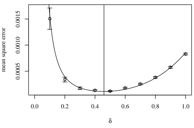
Our second experiment validates the statement of theorem3.3, by numerically estimating the optimal choice of delta and the corresponding MSE.

For fixed values of expected computational cost andδ, we estimate the mean squared error by generatingkdifferent ABC estimates and taking the mean of their squared distance from the true posterior expectation. This reflects how the bias is estimated in experiment 1. Repeating this procedure for several values of

δ, the estimates of the MSE are plotted againstδ.

Our aim is to determine the optimal value ofδfor fixed computational cost. From lemma3.7we know that the expected cost is of ordernδ−q _{and thus we}

choosen_∼δ2 _{in this example. From lemma3.6we know that bias}

∼δ2_{. Thus,} we expect the MSE for constant expected cost to be of the form

MSE(δ) =Var

n + bias

2_=aδ−2_+bδ4 ₍₂₀₎

for some constantsaandb. Thus, we fit a curve of this form to the numerically estimated values of the MSE. The result of one such simulation, usingk= 500 samples for eachδ, is shown in figure 2. The curve fits the data well.

●

●

● _●

● ●

● ●

● ●

0.0 0.2 0.4 0.6 0.8 1.0

0.0005

0.0010

0.0015

δ

mean square error

Fig 2_{. The estimated MSE as a function of the tolerance}δfor fixed expected cost. The fitted curve has the form given in equation(20). The location of the optimalδis marked by the vertical line.

the predicted form (20) of the curve and the empirical MSE values, this procedure promises to be a robust way to estimate the optimal value of δ. The direct approach would likely require a much larger number of samples to be accurate. Repeating the above procedure for a range of values of expected cost gives corresponding estimates for the optimal values ofδand the MSE as a function of expected cost. We expect the optimalδ and the MSE to depend on the cost likex=A_·costB_{. To validate the statements of theorem 3.3 we numerically}

estimate the exponentB from simulated data. The result of such a simulation is shown in figure3. The data are roughly on straight lines, as expected, and the gradients are close to the theoretical gradients, shown as smaller lines. The numerical results for estimating the exponentB are given in the following table.

Plot Gradient Standard error Theoretical gradient

δ ₋0.167 0.0036 ₋1/6_{≈ −}0.167 MSE ₋0.671 0.0119 ₋2/3_{≈ −}0.667

The table shows an an excellent fit between empirical and theoretically predicted values.

6. Discussion

●

●

●

●

●

●

●

●

●

1 2 5 20 50 200

0.4

0.5

0.6

0.7

expected cost

δ

●

●

●

●

●

●

●

●

●

1 2 5 20 50 200

5e−05

2e−04

1e−03

expected cost

MSE

Fig 3_{. Estimated dependency of the optimal}δand of the corresponding MSE on the computa-tional cost. The computacomputa-tional cost is given in arbitrary units, chosen such that the smallest sample size under consideration has cost1. Log-log plots are used so that the theoretically expected relations correspond to straight lines. For comparison, the additional line above the fit has the gradient expected from the theoretical results.

Our results can be applied directly in cases where a pilot run is used to tune the algorithm. In this pilot run the toleranceδ could, for example, be chosen as some quantile of the distances of the simulated summary statistics from the observed summary statistics.

Now assume that the full run is performed by increasing the number of accepted ABC samples by a factor ofk. From theorem3.3we know that optimal performance of the ABC algorithm is achieved by choosingδ proportional to

n−1/4_{. Consequently, rather than re-using the same quantile as in the trial run,} the tolerance δ for the full run should be divided by k1/4_{. In this case the} expected running time satisfies

cost∼nδ−q∼n(q+4)/4

and, using lemma3.7, we have

error_∼cost−2/(q+4)

∼n−1/2_. There are two possible scenarios:

• If we want to reduce the root mean-squared error by a factor of α, we should increase the numbernof accepted ABC samples byα2 _{and reduce} the toleranceδ by a factor of (α2₎1/4₌√_{α. These changes will increase} the expected running time of the algorithm by a factor ofα(q+4)/2_.

and divideδbyβ1/(q+4). These changes will reduce the root mean squared error by a factor ofβ2/(q+4)_.

These guidelines will lead to a choice of parameters which, at least asymptotically, maximises the efficiency of the analysis.

Acknowledgements.The authors thank Alexander Veretennikov for pointing out that the Lebesgue differentiation theorem can be used in the proof of proposition3.1. MW was supported by an EPSRC Doctoral Training Grant at the School of Mathematics, University of Leeds.

References

M. A. Beaumont. Approximate Bayesian computation in evolution and ecology.

Annual Review of Ecology, Evolution, and Systematics, 41:379–406, December 2010.

G. Biau, F. C´erou, and A. Guyader. New insights into approximate Bayesian computation. Annales de l’Institut Henri Poincar´e, 2013. In press.

M. G. B. Blum. Approximate Bayesian computation: A nonparametric perspec-tive. Journal of the American Statistical Association, 105(491):1178–1187, September 2010.

M. G. B. Blum and O. Fran¸cois. Non-linear regression models for Approximate Bayesian Computation. Statistics and Computing, 20:63–73, 2010.

M. G. B. Blum and V.-C. Tran. HIV with contact tracing: a case study in approximate Bayesian computation. Biostatistics, 11(4):644–660, 2010. P. Bortot, S. G. Coles, and S. A. Sisson. Inference for stereological extremes.

Journal of the American Statistical Association, 102(477):84–92, 2007. A. Dembo and O. Zeitouni. Large Deviations Techniques and Applications,

volume 38 of Applications of Mathematics. Springer, second edition, 1998. C. C. Drovandi and A. N. Pettitt. Estimation of parameters for macroparasite

population evolution using approximate Bayesian computation. Biometrics, 67(1):225–233, 2011.

N. J. R. Fagundes, N. Ray, M. Beaumont, S. Neuenschwander, F. M. Salzano, S. L. Bonatto, and L. Excoffier. Statistical evaluation of alternative models of human evolution. Proceedings of the National Academy of Sciences, 104(45): 17614–17619, 2007.

P. Fearnhead and D. Prangle. Constructing summary statistics for approximate Bayesian computation: semi-automatic approximate Bayesian computation.

Journal of the Royal Statistical Society: Series B, 74(3):419–474, 2012. T. Guillemaud, M. A. Beaumont, M. Ciosi, J.-M. Cornuet, and A. Estoup.

Inferring introduction routes of invasive species using approximate Bayesian computation on microsatellite data. Heredity, 104(1):88–99, 2010.

J.-M. Marin, P. Pudlo, C. P. Robert, and R. J. Ryder. Approximate Bayesian computational methods. Statistics and Computing, 22(6):1167–1180, 2012. P. Marjoram, J. Molitor, V. Plagnol, and S. Tavar´e. Markov chain Monte Carlo

without likelihoods. Proceedings of the National Academy of Sciences, 100(26): 15324–15328, 2003.

R Core Team. R: A Language and Environment for Statistical Computing. R Foundation for Statistical Computing, Vienna, Austria, 2013.

O. Ratmann, C. Andrieu, C. Wiuf, and S. Richardson. Model criticism based on likelihood-free inference, with an application to protein network evolution.

Proceedings of the National Academy of Sciences, 106(26):10576–10581, 2009. W. Rudin. Real and Complex Analysis. McGraw-Hill, third edition, 1987. D. Silk, S. Filippi, and M. P. H. Stumpf. Optimizing threshold-schedules for

sequential approximate Bayesian computation: applications to molecular sys-tems.Statistical Applications in Genetics and Molecular Biology, 12(5):603–618, September 2013.

S. Sisson, Y. Fan, and M. M. Tanaka. Sequential Monte Carlo without likelihoods.

Proceedings of the National Academy of Sciences, 104(6):1760–1765, 2007. A. Sottoriva and S. Tavar´e. Integrating approximate Bayesian computation

with complex agent-based models for cancer research. In Y. Lechevallier and G. Saporta, editors,Proceedings of COMPSTAT’2010, pages 57–66. Springer, 2010.

M. M. Tanaka, A. R. Francis, F. Luciani, and S. A. Sisson. Using approximate Bayesian computation to estimate tuberculosis transmission parameters from genotype data. Genetics, 173(3):1511–1520, 2006.

S. Tavar´e, D. J. Balding, R. C. Griffiths, and P. Donnelly. Inferring coalescence times from DNA sequence data. Genetics, 145(2):505–518, 1997.

K. Thornton and P. Andolfatto. Approximate Bayesian inference reveals evidence for a recent, severe bottleneck in a Netherlands population of Drosophila melanogaster. Genetics, 172(3):1607–1619, 2006.

J. Voss.An Introduction to Statistical Computing: A Simulation-Based Approach. Wiley Series in Computational Statistics. Wiley, 2014. ISBN 978-1118357729. D. M. Walker, D. Allingham, H. W. J. Lee, and M. Small. Parameter inference in small world network disease models with approximate Bayesian computational methods. Physica A, 389(3):540–548, 2010.

D. Wegmann and L. Excoffier. Bayesian inference of the demographic history of chimpanzees. Molecular Biology and Evolution, 27(6):1425–1435, 2010. R. D. Wilkinson. Approximate Bayesian computation (ABC) gives exact results

under the assumption of model error. Statistical Applications in Genetics and Molecular Biology, 12(2):129–141, 2013.