On numerical issues for the wave/finite element method

(1)

On Numerical Issues for the Wave/Finite Element Method

Y. Waki, B.R. Mace and M.J. Brennan

(2)

SCIENTIFIC PUBLICATIONS BY THE ISVR

Technical Reports are published to promote timely dissemination of research results by ISVR personnel. This medium permits more detailed presentation than is usually acceptable for scientific journals. Responsibility for both the content and any opinions expressed rests entirely with the author(s).

Technical Memoranda are produced to enable the early or preliminary release of information by ISVR personnel where such release is deemed to the appropriate. Information contained in these memoranda may be incomplete, or form part of a continuing programme; this should be borne in mind when using or quoting from these documents.

Contract Reports are produced to record the results of scientific work carried out for sponsors, under contract. The ISVR treats these reports as confidential to sponsors and does not make them available for general circulation. Individual sponsors may, however, authorize subsequent release of the material.

COPYRIGHT NOTICE

(3)

UNIVERSITY OF SOUTHAMPTON

INSTITUTE OF SOUND AND VIBRATION RESEARCH

DYNAMICS GROUP

On Numerical Issues for the Wave/Finite Element Method

by

Y. Waki, B.R. Mace and M.J. Brennan

ISVR Technical Memorandum No: 964

December 2006

Authorised for issue by Professor M.J. Brennan

Group Chairman

(4)

ABSTRACT

The waveguide finite element (WFE) method is a numerical method to investigate wave

motion in a uniform waveguide. Numerical issues for the WFE method are specifically

illustrated in this report. The method starts from finite element mass and stiffness matrices of

only one element of the section of the waveguide. The matrices may be derived from

commercial FE software such that existing element libraries can be used to model complex

general structures. The transfer matrix, and hence the eigenvalue problem, is formed from the

dynamic stiffness matrix in conjunction with a periodicity condition. The results of the

eigenvalue problem represent the free wave characteristics in the waveguide. This report

concerns numerical errors occurring in the WFE results and proposing approaches to improve

the errors.

In the WFE method, numerical errors arise because of (1) the FE discretisation error, (2)

round-off errors due to the inertia term and (3) ill-conditioning. The FE discretisation error

becomes large when element length becomes large enough compared to the wavelength.

However, the round-off error due to the inertia term becomes large for small element lengths

when the dynamic stiffness matrix is formed. This tendency is illustrated by numerical

examples for one-dimensional structures.

Ill-conditioning occurs when the eigenvalue problem is formed and solved and the resulting

errors can become large, especially for complex structures. Zhong’s method is used to

improve the conditioning of the eigenvalue problem in this report. Errors in the eigenvalue

problem are first mathematically discussed and Zhong’s method validated. In addition,

singular value decomposition is proposed to reduce errors in numerically determining the

eigenvectors. For waveguides with a one-dimensional cross-section, the effect of the aspect

ratio of the elements on the conditioning is also illustrated. For general structures, there is a

crude trade-off between the conditioning, the FE discretisation error and the round-off error

due to the inertia term. To alleviate the trade-off, the model with internal nodes is applied. At

low frequencies, the approximate condensation formulation is derived and significant error

reduction in the force eigenvector components is observed.

Three approaches to numerically calculate the group velocity are compared and the finite

difference and the power and energy relationship are shown to be efficient approaches for

(7)

1. INTRODUCTION

1.1 Introduction

The waveguide finite element (WFE) method is a useful method when the dynamic behaviour of a uniform structure is of concern. The method involves the reformulation of the dynamic stiffness matrix, which includes the mass and stiffness matrices of a section of the structure, into the transfer matrix. Structural wave motion is expressed in terms of the eigenvalues and the eigenvectors of this matrix and these represent the wavenumbers and the wave modes respectively. However, several numerical difficulties arise when the problem is reformulated from a conventional finite element (FE) model. The aim of this report is (1) to identify and quantify the potential numerical problems and (2) to suggest alternative ways of determining the wave properties of a structure such that the numerical errors are reduced.

1.2 Overview of Periodic Structure Analysis

Many structures have uniformity or periodicity in certain directions. To analyse such structures, Floquet theory [1], which is one of the basic theories of wave propagation in periodic structures, or the transfer matrix method e.g. [2] can be used. The basic idea is that the propagation properties of waves in a periodic structure can be obtained from the propagation constants or by the transfer matrix. Although most of the early papers give the analytical dispersion relationship for relatively simple structures [3,4], numerical calculation is generally needed for complex structures. For complex structures, the finite element method (FEM) may be applied to calculate the propagation constants [5,6,7]. The transfer matrix is formed from the mass and stiffness matrices of discretised elements and the wave propagation characteristics are then described by the eigenvalues and eigenvectors of the transfer matrix.

(8)

results for simple structures and Hinke et al [15] analysed wave properties in a sandwich panel. Mencik [16] formulated the problem of wave coupling between two general substructures and Maess [17] analysed a fluid filled pipe using an eigenpath analysis. One of the advantages of the WFE method is the computational cost [18] since this method needs information drawn from only one small section along the direction which the waves propagate. Another possible way of analysing such structures is the spectral finite element method [19] which uses a special shape function to represent the motion of a cross-section of the structure. However, this method needs special shape functions and element matrices to be developed for different wave types.

The WFE method needs only the conventional mass and stiffness matrices of a structure. Since the standard FE-package can be utilised to generate the stiffness and mass matrices, the full power of existing element libraries can be employed. In addition, since the wave characteristics are calculated for a given frequency, nearfield and oscillating decaying waves, which might be important for the system response near excitation points or discontinuities, can be effectively included. The forced response can be calculated using the wave approach (e.g. [20]).

1.3 Outline of the Report

The wave motion could be derived from the eigenvalues and eigenvectors of the transfer matrix. However, numerical difficulties may be encountered when solving the eigenvalue problem. Most papers mention the matrix conditioning of the eigenvalue problem [9,10,11,13,14,17] but do not discuss many details.

(9)

2. OVERVIEW OF THE WAVEGUIDE FINITE

ELEMENT METHOD

2.1 Introduction

In this section, a brief overview of the WFE formulation is given. A small section of a structure is first modelled using FE. From the dynamic stiffness matrix of the elements the transfer matrix is formed. The transfer matrix describes the wave motion through the element and the eigenvalues and the eigenvectors of the resulting eigenvalue problem represent the wavenumbers and the wave modes in the structure.

2.2 Finite Element Formulation of a Structural Element

The equation of motion for uniform structural waveguides can be expressed as

+ + =

Mq Cq Kq f (2.1)

where M, K, and C are the mass, stiffness and damping matrices respectively, f represents the loading vector and q is the vector of the nodal displacement degrees of freedom (DOFs). Throughout this report, time harmonic motion ej tω is implicit. Equation (2.1) then becomes

(

2

)

j

ω ω

= − + + =

Dq M C K q f (2.2)

where D is the dynamic stiffness matrix. The nodal forces and DOFs are decomposed into sets associated with the left (L), right (R) cross-section and interior (I) nodes. For the case where there are no external forces on the interior nodes, equation (2.2) can be partitioned into

LL LR LI L L RL RR RI R R IL IR II I

     

     ₌

     

     

D D D q f

D D D q 0

(2.3)

which may be expressed as

MM MI M M IM II I

     

=

     

 

   

D D q f

D D q 0 (2.4)

(10)

1 I II IM M

− = −

q D D q (2.5)

such that

1 M

M M

I II IM −

   

= =

  ₋ 

   

q I

q Rq

q D D (2.6)

where I is the identity matrix. Using the matrix R in equation (2.6), equation (2.4) becomes

T MM MI

M M IM II

 

=

 

 

D D

R Rq f

D D . (2.7)

Expanding equation (2.7) leads to

1

MM MI II IM M M −

 −  =

D D D D q f (2.8)

such that DOFs associated with internal nodes can be eliminated.

If the group velocity is calculated from the power flow and energy relationship stated later in this section, the form of equation (2.7) is useful to derive the reduced M K, and C

matrices. Putting these matrices instead of D into equation (2.7) readily gives the reduced matrices. The reduced mass matrix is, for example,

T 1 1 1 1

MM MI II IM MI II IM MI II II II IM

− − − −

= − − +

R MR M D D M M D D D D M D D . (2.9)

After removing internal DOFs, equation (2.2) for the section can be written as

LL LR L L RL RR R R

     

=

     

     

D D q f

D D q f . (2.10)

For a uniform section, the following relationships hold:

T T T

, ,

LL = LL RR= RR LR = RL

D D D D D D (2.11)

and

sgn , sgn

RRij = ⋅ LLij RLij = ⋅ LRij

D D D D (2.12)

where ⋅T indicates the transpose and the signs in equations (2.12) depend on whether DOFs at the element interface are symmetric or anti-symmetric [9].

2.3 Wave Basis

(11)

2.3.1 Transfer Matrix

The transfer matrix can be defined on the basis of the continuity of displacements and the equilibrium of forces of adjacent elements as [1]

L R

    =   ₋     

q q

T

f f (2.13)

where T is the transfer matrix. The transfer matrix can be formed from the elements of the dynamic stiffness matrix as [13]

1 1

LR LL LR RL RR LR LL RR LR

− −

 − 

= ₋ ₊ ₋ 

 

D D D

T

D D D D D D . (2.14)

From a periodicity condition [1], free wave motion over the element length ∆ is described in the form of an eigenvalue problem such that

λ

   

=        

q q

T

f f . (2.15)

Although equation (2.15) formulates the basic principle for the WFE method, this eigenvalue problem is likely to be ill-conditioned for general problems because of the ill-conditioning of

LR

D and the fact that the elements of the eigenvector range over a large magnitude. The conditioning of the eigenvalue problem is described in Section 3.

2.3.2 Eigenvalues and Eigenvectors

The eigenvalues

λ

_i_{in equation (2.15) relate to wave propagation over the distance}∆_such that [1]

i

jk i e λ ₌ − ∆

(2.16)

where k_i represents the wavenumber for the ith wave. The wavenumber can be purely real, purely imaginary or complex, associated with a propagating, a nearfield (evanescent) or oscillating decaying wave respectively. The eigenvector corresponding to the ith eigenvalue can be expressed as

i i

i   =    

q Φ

f . (2.17)

The eigenvector represents a wave mode and contains information about both the displacements and the internal forces. For uniform waveguides, there exist positive and negative going wave pairs in the form of jki

i e λ± ₌ ± ∆

(12)

eigenvectors are expressed as

(

λ_i,Φ_i+

)

and

(

1λ_i,Φ_i−

)

. Positive-going waves are those for which the magnitude of the eigenvalues is less than 1, i.e.

λ

_i <1 or if

λ

_i =1, such that the

power is positive going, i.e.

{ }

H

{

H

}

Re f q =Im ωf q >0 [13,14] where _⋅H

represents the

complex conjugate transpose or Hermitian.

2.4 Group Velocity

The group velocity is the velocity at which the wave propagates. The group velocity for the

ith wave is defined by (e.g. [21])

gi i c k ω ∂ =

∂ . (2.18)

There are several approaches to the numerical calculation of the group velocity.

The finite difference method calculates the group velocity from a first order approximation as ( ) ( ) ( ) ( ) ( ) 1 1 1 1 n n n

gi n n i i

c

k k

ω

+

ω

−

+ −

− =

− (2.19)

where n-1, n, n+1 are consecutive discrete frequencies. Other definitions for equation (2.19) are possible. Once the dispersion relationship is determined, the group velocity can be obtained.

Another approach for the group velocity is in terms of the power and energy as [21]

, i gi tot i P c E = (2.20)

where P is the time average power transmission thorough the cross section of a waveguide and Etot is the total energy density. These values are given by [14,21]

{ }

H

{ }

H 1

Re Im

2 2

i i i i i

P = f q =ω f q . (2.21)

and

{

}

{

}

{

}

, , ,

2

H H H

, ,

,

1 1

Re Re , Re

4 4 4

tot i k i p i

k i i i i i p i i i

E E E

E

ω

E

= +

= = − =

∆ q Mq ∆ q Mq ∆ q Kq

(2.22)

(13)

In addition, the group velocity could be determined directly by differentiating the eigenproblem [22]. The group velocity can be expressed as

2 1 2 gi i i c k k

ω

∂ ∂ = =

∂ ∂ (2.23)

and ∂ ∂k

ω

2 is found from the differentiation of the eigenvalue problem (2.15) such that

( )

ω2

{

(

λ

)

i

}

∂ ₋ ₌

∂ T I Φ 0. (2.24)

Expanding equation (2.24), using equations (2.16), (2.23) and premultiplying by the left eigenvector Ψi leads to

( )

2 0

2

i

i i i

k j

λ

ω

 _∂ _∆ _∂   +  = ∂ ∂   

Ψ T I Φ . (2.25)

Recalling equation (2.14), noting the differentiation of the matrix inverse [23],

( )

2 LR1 LR1 LR LR1 ω

− − −

∂ _{= −}

∂ D D M D ,

( )

2

ω

∂ ∂T in equation (2.25) can be evaluated as

( )

1 1 1 1 1

1

1 1 1

2

1 1 1

LR LR LR LL LR LL LR LR LR RL RR LR LL

RR LR RR LR LR LR RR LR LR LR LL RR LR LL

ω − − − − − − − − − − − −  − +    ∂ ₌ − +  ₋  ∂ _ _ −  

D M D D D M D M D

T M M D D

M D D D M D

D D M D D D D M

. (2.26)

From the above equations the group velocity is given by

( )

2 2

i i i gi i i j c λ ω ω ∆ = − _∂ ∂ Ψ IΦ Ψ TΦ

. (2.27)

(14)

3. NUMERICAL ISSUES AND

IMPLEMENTATION

3.1 Introduction

In this section, the conditioning of the eigenvalue problem is illustrated. Numerical errors occurring in the eigenvalue problem are mathematically explained and the conditioned eigenvalue problem is introduced. In particular, the singular value decomposition (SVD) is applied to reduce errors for numerically determining the eigenvectors. Numerical errors in the WFE method are then enumerated.

3.2 Conditioning of the Eigenvalue Problem

The eigenvalue problem was formulated using the transfer matrix (2.15). However, the results from the eigenvalue problem might be inaccurate. In this section the conditioned eigenvalue problem is introduced and SVD application is proposed to reduce numerical inaccuracies for determining the eigenvectors.

3.2.1 Mathematical Background of Numerical Errors in the

Eigenvalue Problem

Numerical errors occur (1) when the eigenvalue problem is formulated and (2) when the eigenvalue problem is solved. When the eigenvalue problem (2.14) is formulated, numerical errors can arise predominantly from the matrix inversion. The maximum resulting errors for the matrix inversion A−1 can be of the order of

ε κ

⋅

( )

A where

ε

is the machine precision and

( )

1

max min

κ ₌ − ₌σ σ

A A A (3.1)

(15)

matrix approach (2.15) is formed, D_LR−1 should be calculated which in general might be ill-conditioned. This causes numerical errors when the eigenvalue problem is formed.

Next, numerical errors occurring in the solution of the eigenproblem are discussed. The matrix for the eigenvalue problem in the WFE method is square, complex and non-symmetric. For such matrix Schur factorisation is known to be most useful in numerical analysis because all matrices, including defective ones, can be factored in this way [24]. Major software packages such as MATLAB and Mathematica use Schur factorisation for solving such eigenvalue problems.

Many different approaches for assessing the error bounds on the computed eigenvalues and eigenvectors have been proposed, e.g. [26,27]. A well-known estimate for the error bound is given by Gerschgorin’s theorem [24]. However, this theorem usually gives a large error bound for an ill-conditioned matrix. More precisely, the following discussion holds for Schur factorisation [25].

When the eigenvalue problem AΦ=λΦ or Ψ AH =λΨH is solved using Schur factorisation, the matrix A is factorised into the form Q AQH = +D N where Q is unitary, D

is diagonal and N is strictly upper-triangular [25]. The resulting errors for the eigenvalue problem are estimated from

κ

( )

Q or N [25]. If

κ

( )

Q is large then the eigenvector matrix

is ill-conditioned. If the eigenvectors are far from orthogonal to each other, the results may contain large errors [24,25]. Since the eigenvectors in the transfer matrix approach (2.15) contains both the displacement and force components and usually each eigenvector is far from orthogonal to each other,

κ

( )

Q is likely to be issue for general cases. A large value for N

means that A is far from normal, e.g. strongly asymmetric [25]. Such eigenvalue problems are likely to have a large error in the computed results, which is the case for the transfer matrix approach stated in equation (2.14).

Specifically, for n≥5 for the n n× matrix A, there is no analytical expression for the roots of the characteristic polynomial so that the eigensolver must be iterative [24]. For a matrix of large size, conditioning becomes more important for errors when Schur factorisation is applied to solve the eigenvalue problem. In this report, the matrix size for a rod and a beam is

2, 4

n= respectively such that conditioning effects are small. However, the conditioning becomes important for a plate example as the matrix size becomes large.

(16)

( )

2 1

1 i

s λ

≤

− Ε

A (3.2)

where Ε is the perturbation matrix incurred from the round-off error because of the finite digit arithmetic and s

( )

λ

_i is the sensitivity of the eigenvalue with respect to the perturbation, given by [25]

( )

H

( ) ( )

1 1

i i i

s

λ

= Ψ

λ

Φ

λ

≥ (3.3)

with Φi = Ψi =1. Under the condition (3.2), two distinct but similar eigenvalues λ λi, j

become repeated eigenvalues

λ λ

_i', '_j whose values are different from both λ_i and λ_j [25]. Examples using MATLAB eigenvalue solvers can be found in [28,29].

3.2.2 Overview of the Conditioning for the Eigenvalue Problem

To improve the ill-conditioned problem (2.15), several works [10,13,14,15,16] applied Zhong’s algorithm [30]. The details can be seen in [30,31,32]. This method formulates the conditioned, general eigenvalue problem such that D_LR is not necessarily inverted. In addition,

since the eigenvector contains only displacement components, numerical error could be reduced because

κ

( )

Q can be smaller. Thompson [9] also derived the similar eigenvalue

problem using symmetric relationships, e.g. equations (2.11), (2.12), which results in smaller size of the eigenvalue problem.

In this report, Zhong’s algorithm has been applied because the approach seems well matched with the problems which have been considered so far.

3.2.3 Zhong’s Method and Practical Implementation

Zhong’s method [30] is illustrated in this section. The method starts from a reformulation of equation (2.13) into the relationships for the displacement vectors alone:

,

L n L R n L

L LL LR R R RL RR R

           

= =

        ₋ ₋   

           

q I 0 q q 0 I q

f D D q f D D q . (3.4)

After some matrix operations using the periodicity condition and the symplectic relationship [30], equations (3.4) can be rearranged as

,

RL LL RR L LR L

RL L RL L

λ

− − −

       

=

 ₋    ₋   

       

D D D q 0 D q

(17)

and

1

.

LR L LR L

RR LL LR

λ

L

λ

RL

λ

L

       

=

 ₊    ₋   

       

D 0 q 0 D q

D D D q D 0 q (3.6)

Adding equations (3.5) and (3.6) gives the general eigenvalue problem:

1 2 µ λ λ     =         q q Z Z

q q (3.7)

with

(

)

(

)

(

) (

)

1 , 2

LR RL LL RR LR

LL RR LR RL RL − − +     =_ _ _{= } _ + − −    

D D D D

0 D

Z Z

D D D D

D 0 (3.8)

where

µ λ

= +1

λ

and the subscript L for the eigenvector is suppressed for clarity. For symmetric elements, several elements of Z₂ in equation (3.7) cancel each other as certain relationships (2.11), (2.12) hold and Z₁ and Z₂ in equation (3.7) become skew-symmetric. In practice, it is recommended that either Z₁ or Z₂ is inverted such that the standard eigenvalue problem 1 1 2 µ λ λ −     =         q q Z Z

q q or

1 2 1 1 λ λ µ −     =         q q Z Z

q q (3.9)

is formulated. To reduce numerical errors, the matrix with the smaller condition number should be inverted [33]. In addition, the pseudo matrix inverse (e.g. [24]) can be applied to reduce numerical errors.

One might be interested in only several waves with small wavenumbers. A limiting case is when a wave is at the cut-off frequency (usually k →0) such that usually

µ λ

= +1

λ

→2. In such cases, it is beneficial to take the form of µ−2

(

or 1

µ

−0.5

)

rather than µ

(

1

µ

)

in equations (3.9) such that the important eigenvalues can be bounded by several smallest (largest) values.

Equations (3.9) are a standard, double eigenvalue problem whose eigenvectors contain only the displacement components. The original eigenvalues λ_i,1λ_i can be determined from the

calculated eigenvalue µ_i =λ_i+1 λ_i by solving the quadratic equation or by using a trigonometric function of the form 1 jki jki 2 cos

( )

i i i e e ki

µ

₌

λ

₊

λ

₌ − ∆ ₊ ∆ ₌ _∆

.

(18)

1,2 1,2 1,2

λ

  =     q φ

q . (3.10)

The original eigenvector associated with eigenvalues λ_i,1λ_i can be found from a linear

combination of φ φ₁, ₂ [13,14,30], i.e.,

1 1 2 2

α α λ   =_ _= +   q

φ φ φ

q . (3.11)

Substituting equations (3.11) and (3.10) into equation (3.5) gives

1 2

RL LL RR LR

RL RL

λ

α

λ

  − − − −    ₊  ₌    ₋             

D D D D q q

0

D D q q . (3.12)

Taking the scalar product of φ₁H leads to the relationship between

α

₁ and

α

₂ such that [13] 1 H H 1 1 1 2 2 H H 1 1 1 2 RL LL RR LR

RL RL

RL LL RR LR

RL RL

λ

α

λ

α

λ

− − − −      _{ } _{ } _   ₋     = − − − − −      _{ } _{ } _   ₋    

D D D D q

q q

D D q

D D D D q

q q

D D q

. (3.13)

Although equation (3.13) is algebraically correct, there may be some difficulties when calculating it numerically. In the next section, an alternative way of determining the eigenvectors is investigated using singular value decomposition (SVD).

3.2.4 Application of SVD for Determination of Eigenvectors

The eigenvectors could be obtained from equation (3.13) but numerical problems may occur. For the limiting case λ→1, equation (3.13) approaches

α α

2 1→0 0 and round-off errors during arithmetic calculations become large.

Alternatively, SVD may be applied. Equation (3.12) can be written in another form as

1 2 1

1 2 2

RL LL RR LR

RL RL

λ

α

λ

α

− − − −

     

=

 ₋     

     

D D D D q q

0

D D q q . (3.14)

Writing equation (3.14) as A

[

α

₁

α

₂

]

T =0 with an n×2 rectangular matrix A, where n is the length of the eigenvector, the problem is now to solve an overdetermined simultaneous equation if n≥3. SVD can be applied to solve an overdetermined linear equation [34]. Performing SVD on A gives

H =

(19)

where the matrix dimensions are A∈

(

n×2 ,

)

U∈

(

n n×

)

,S∈

(

n×2 ,

)

V∈

(

2 2×

)

. Equation (3.15) can be written as

( )

T 1

11 12 21 22

0 0 0

0 0 0 0

v v

v v _ε

σ

    =     _≈     A U

. (3.16)

The matrix S contains two singular values on its leading diagonal and one of these is almost zero. The second column of equation (3.16) and expanding A to the original expression gives

1 2 12 1 2 22 RL LL RR LR

RL RL

v v

λ

− − − −

     

≈

 ₋     

     

D D D D q q

0

D D q q (3.17)

such that

[

α

₁

α

₂

]

T are given by

2 22 1 21

v v

α

= . (3.18)

The advantages of SVD approach are

(1) equation (3.18) can be derived from only one matrix multiplication while equation (3.13) needs two multiplications for both the denominator and numerator such that numerical errors through the matrix operations can be reduced and,

(2) the orders of v21,v22 in equation (3.18) are typically O

( )

1 while that of the original values

α α

₁, ₂ in equation (3.13) may be very small.

After finding the vector of displacements from equations (3.11) and (3.18), the corresponding force eigenvector can be calculated from the first row of equation (2.15) as

(

LL

λ

LR

)

= +

f D D q. (3.19)

The original right eigenvector associated with

λ

_i is then

( )

_{( )}

( )

i

₍

( )

i

_{) ( )}

i i

i LL i LR i

λ

    = =_ _{ }= _ +     q q Φ Φ

f D D q . (3.20)

Similarly, the original left eigenvector can be obtained as [13]

( )

(

) (

_T

)

(

)

T

1 1

i =

λ

i =_

λ

i RR+

λ

i LR

λ

i _

Ψ Ψ q D D q . (3.21)

3.3 Numerical Errors in the WFE Method

(20)

3.3.1 Errors in the Conditioned Eigenvalue Problem

The sequential procedure for the WFE method, based on the conditioned eigenvalue problem, can be illustrated as follows. The damping matrix C is excluded for simplicity.

(1) Discretise a section of a structure of length ∆ using FE such that K, M are formed. (2) Calculate the dynamic stiffness matrix D=K−

ω

2M for each frequency.

(3) Formulate the standard eigenvalue problem, i.e. equation (3.9). (4) Solve the eigenvalue problem.

(5) Calculate the original eigenvalues and eigenvectors, i.e. equations (3.11) and (3.18). (6) Calculate the force components from equation (3.20).

For steps (3)-(5), the conditioning is essential to reduce numerical errors for a matrix of large size. For step (1), the FE discretisation error should be first considered and specifically for step (2), the round-off error can be important. Each error is explained.

3.3.2 FE Discretisation Error

When a structure is discretised using FE, FE discretisation errors occur. To represent the system motion accurately, 6 or more FE are generally needed for each wavelength [35]. In the WFE formula, this criterion can be expressed as [13]

1

k∆ ≤ . (3.22)

Equation (3.22) should be satisfied both along the waveguide and over its cross-section. For accurate results, small ∆ is needed for large wavenumbers. However, very small ∆ is inappropriate because the conditioning is likely to deteriorate and the round-off error due to the inertia term increases. The section length ∆ should be carefully determined when the structure is modelled. Examples will be shown in Sections 4 and 5.

3.3.2 Round-Off Errors in the Dynamic Stiffness Matrix

The round-off errors occur in every numerical arithmetic operation. Specifically, this error can be important when the dynamic stiffness matrix, ₌ ₋

ω

2

D K M, is numerically calculated. The error becomes large when K_ij

ω

2M_ij because of the finite precisions of arithmetic operations.

It should be noted that the criteria where the round-off errors become large depends not

(21)

D becomes inaccurate such that the eigenvalue problem cannot be accurately formed. To

evaluate the round-off error due to the inertia term,

(

2

)

min

ω

M_ii K_ii may be a indication

since some off-diagonal terms may not be important. To reduce this error, ∆ should not be too small when the structure is modelled.

(22)

4. NUMERICAL EXAMPLES OF A ROD AND A

BEAM

4.1 Introduction

The quasi-longitudinal waves in a rod and flexural waves in a beam are considered. The accuracy of results calculated by the WFE method is discussed in this section. No damping is assumed.

4.2 Quasi-Longitudinal Waves in a Rod

The quasi-longitudinal waves in a rod are considered in this section. The WFE results are compared with the analytical solution and the accuracies are evaluated.

4.2.1 Discretisation of a Rod Element

The mass and stiffness matrices for the rod element can be modelled using a linear shape function such that [35]

1 1

EA − 

= _ _

−

∆  

K , 2 1

1 2 6

A

ρ

∆ 

= _ _

 

M (4.1)

where E is the Young’s modulus, A is the cross-sectional area,

ρ

is the mass density and ∆ is the length of a section. The dynamic stiffness matrix, D=K−

ω

2M, then becomes

(

)

(

)

(

)

2 2

2

1 1

3 6

. 1

3

L L

L

k k

EA

k sym

 _∆ _∆ 

− − −

 

=

 

∆ _∆

 − 

 

D (4.2)

where

L

k =

ρ ω

E (4.3)

is the quasi-longitudinal wavenumber [36]. The dynamic stiffness matrix in equation (4.2) is

(23)

(

)

{

4

}

L

O k ∆ for small k_L∆. The transfer matrix (2.14) can be obtained from equation (4.2) [13] such that

(

)

(

)

(

) (

)

(

)

2 4 2 2 2 1 3 1 1 1 12 3 6 L L L L L k EA k k EA k k  _∆ _∆  − −     = _ _ _ _ ∆ ∆ ∆ _  _{∆ −}  ₋ _ + _   _ ∆ _ _  

T . (4.4)

4.2.2 Analytical Expressions for the Eigenvalues and Eigenvectors

The analytical solution for the WFE formulation can be found from equation (4.4). The eigenvalues are analytically given as [13]

(

)

(

)

2

₍

₎

(

)

2 2 1 1 1 3 12 1 6 L L L L k k j k k

λ

± ₌  ₋ ∆ _∆ ₋ ∆ 

 

∆ _ _

+

∓ . (4.5)

For small kL∆, equation (4.5)can be expanded to

(

)

2

(

)

3 5 1 2 24 L L L k k jk j

λ

± ₌ _∓ _{∆ −} ∆ _± ∆ ₊

(4.6)

and this is accurate up to O

{

(

k_L∆

)

2

}

with error being O

{

(

k_L∆

)

3

}

. It should be noted that the error in the wavenumber given from log

( )

λ

± − =j k±∆ becomes from equation (4.6)

( )

(

)

2 1 8 L L k

k∆ = ± ∆ +± k  ∆ 

 

 

∓ (4.7)

such that relative error in the wavenumber is O

{

(

k_L∆

)

2

}

.

The right eigenvectors associated with the eigenvalues (4.5) can be analytically obtained as

(

)

2 1 1 12 L u k f _jEAk ±       =_{ }=_ _∆ _   _ − _   Φ ∓ (4.8)

where u is the longitudinal displacement and f is the normal force. The exact solution for a continuous rod is [36]

[

f u

]

± =∓jEAk. (4.9)

(24)

[

]

{

(

)

2

}

1 _L 24

WFE

f u ± =∓jEAk − k ∆ (4.10)

for small k_L∆ with the relative error being O

{

(

k_L∆

)

2

}

.

4.2.3 Relative Errors in the Eigenvalues and Eigenvectors

Figures 4.1, 4.2 show the relative errors in the wavenumber,

(

k−kL

)

kL, and the force eigenvector per unit displacement,

(

f_WFE− f

)

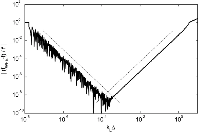
f , respectively. In both figures, the trend of the curve is same. The relative errors increase for k_L∆ > ⋅3 10−4 because of the FE discretisation error and, for k_L∆ < ⋅3 10−4 because of the round-off errors due to the inertia term. Although the size of the error is small for very small k_L∆, it should be noted that not only the magnitude but also the phase of the force eigenvector fluctuates such that the forced response of the system will fluctuate because of the numerical errors. When the forced response at low frequencies is of concern, length of the element ∆ should be chosen as enough large to reduce the round-off errors due to the inertia term.

Asymptotic slopes in the relative errors at large k_L∆ and small k_L∆ are +20 dB/decade and -20 dB/decade, respectively. For large k_L∆, the asymptotic slope is about +20 dB/decade in both figures. This behaviour can be explained from equations (4.7) for the wavenumber (Figure 4.1) and equation (4.10) for the eigenvector (Figure 4.2).

For small k_L∆ , the round-off error is dominant for the relative errors such that the minimum value of

ω

2M_ii K_ii is of concern since some off-diagonal terms may not be important for general cases. From equations (4.1), it is given that min

(

ω

2M_ii K_ii

)

=

(

)

2

1 3 k_L∆ . From this estimation, the round-off error due to the inertia term is related to

(

)

2

L

k ∆ − , which is same as the asymptotic slope in the relative errors. If the ratio is greater than 10 16

(

8

)

10 L

k ∆ < − , all the inertia terms could be rounded in double precision calculation as can be seen in the figures.

(25)

10-8 10-6 10-4 10-2 100 10-10

10-8 10-6 10-4 10-2 100 102

k_L∆

|

(k

-k L

)

/

k L

[image:25.595.117.453.77.302.2]

|

Figure 4.1: Relative error in the wavenumber: ··· asymptote ±20dB decade.

10-8 10-6 10-4 10-2 100

10-10 10-8 10-6 10-4 10-2 100 102

k L∆

|

(f W

F

E

-f

)

/

f

|

Figure 4.2: Relative error in the eigenvector: ··· asymptote ±20dB decade.

4.2.4 Relative Errors in the Group Velocity

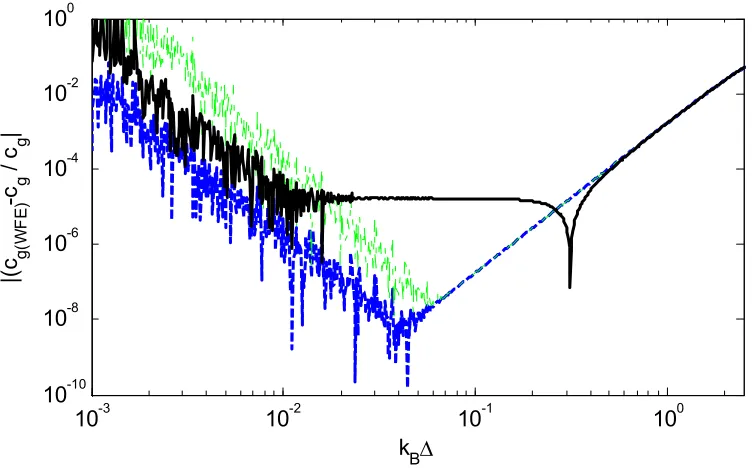
The group velocity is numerically calculated using the approaches illustrated in Section 2.4.

The relative errors in the group velocity

(

c_{g WFE}₍ ₎−c_g

)

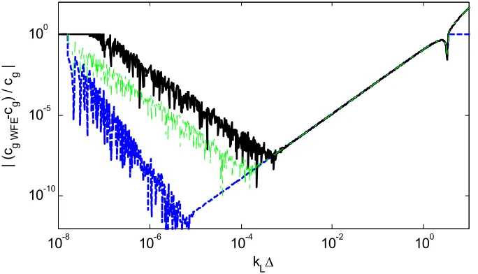
c_g are plotted in Figure 4.3 where c_g

[image:25.595.115.454.361.586.2]

(26)

For all methods, the relative error is almost same above k_L∆ >10−3. The relative error of the power and energy relationship is smallest below k_L∆ <10−3. Since the group velocity is calculated from the power flow and the energy density given in equations (2.21) and (2.22), small fluctuated errors in the eigenvectors can be improved through the calculation. At this frequency range, the relative error for the differentiation of the eigenproblem shows the almost same curve as those in the wavenumber and eigenvector while that the error for the finite difference method is larger very slightly. Although the error for the finite difference method depends on the frequency step, too small frequency step does not always improve the error because the error becomes more sensitive to the errors in the dispersion relationship.

10-8 10-6 10-4 10-2 100

10-10 10-5 100

k L∆

|

(c g

W

F

E

-c g

)

/

c g

|

Figure 4.3: Relative errors in the group velocity: ― finite difference, – – power and energy

relationship, −·− differentiation of the eigenproblem.

4.3 Flexural Waves in an Euler-Bernoulli Beam

The flexural waves in the Euler-Bernoulli beam (e.g. [36]) are considered. The WFE results are evaluated with the analytical solution.

4.3.1 Analytical Expression for the Discretised Beam Element

[image:26.595.115.457.296.492.2]

(27)

2 2

3

2

12 6 12 6

4 6 2

. 12 6

4 EI sym ∆ − ∆    _∆ _{− ∆} _∆    =  − ∆ ∆  _∆    K , 2 2 2

156 22 54 13

4 13 3

. 156 22

420 4 A sym ρ ∆ − ∆    _∆ _{∆ − ∆}  ∆   =  − ∆  _∆    M (4.11)

where EI is the bending stiffness,

ρ

is the mass density and A is the cross-sectional area. The dynamic stiffness matrix then becomes

(

)

(

)

(

)

(

)

(

)

(

)

(

)

(

)

(

)

(

)

4 4 4 4

4 4 4

2 2

3

4 4

4 2

156 22 54 13

12 6 12 6

420 420 420 420

4 13 3

4 6 2

420 420 420

156 22

. 12 6

420 420

4 4

420

B B B B

B B B

B B

B

k k k k

k k k

EI

sym k k

k  ₋ _∆  _∆ ₋ _∆  ₋ ₋ _∆  _∆ ₊ _∆                    _∆  ₋ _∆  _{∆ − −} _∆  _∆  ₊ _∆              = ∆  ₋ _∆  _{∆ − +} _∆            ∆ _ − ∆ _    D                    (4.12) where 4 B A k EI

ρ

_ω

= (4.13)

is the bending wavenumber [36]. The dynamic stiffness matrix in equation (4.2) is accurate

for the analytical dynamic stiffness matrix [37] up to O

{

(

k_B∆

)

4

}

with error being O

{

(

k_B∆

)

8

}

for small kB∆.

(28)

(

) (

)

(

)

(

)

(

)

(

)

(

)

(

)

₍

₎

₍

₎

(

)

(

)

(

)

(

)

(

)

(

)

(

)

4 8

4 8 4 8

4 8

4 8 12 4 8 12

3 2

4

1 302400 720

302400 13320 26 302400 3240 2

50400 120

302400 13320 10

7 1

302400 2820 151200 570

2 4

151200 570

B B

B B B B

B B

B B B B B B

B

k k

k k k k

k k

EI k k k EI k k k

EI k k

= × + ∆ + ∆ + ∆ + ∆ ∆ + ∆ + ∆ ∆ + ∆ + ∆ + ∆ ∆  _{∆ +} _{∆ +} _∆   _{∆ +} _{∆ +} _∆          ∆ ∆ − ∆ − T

(

)

(

)

(

)

(

)

(

)

(

)

(

)

(

)

(

)

(

)

(

)

(

)

(

)

(

)

(

)

(

)

8 12 4 8 12

2 4 4 3 2 4 4 2 4 8 4 8 4 1 1 50400 78 4 60

50400 180 151200 780

151200 780 302400 3240

50400 120

302400 13320 26

302400 3240

B B B B B

B B

B

k EI k k k

k k EI EI k k EI EI k k k k k                _{∆ −} _∆ ₋ _{∆ −} _{∆ −} _∆      _ _ _ _   ∆ ∆ ∆ + ∆ ∆ − − ∆ ∆ + ∆ ∆ − − ∆ − ∆ − ∆ + ∆ + ∆ ∆

∆ −

(

− ∆

(

)

8

)

(

)

4

(

)

8

2 k_B 302400 13320 k_B 10 k_B

           − ∆ + ∆ + _{∆ } .(4.14)

Approximate solutions for the characteristic equation derived from the transfer matrix (4.14) are [13]

(

)

(

)

(

)

(

)

(

)

(

)

(

)

(

)

(

)

(

)

(

)

(

)

2 3 4 5

1,2

2 3 4 5

3,4

1 1 23

1 ,

2 6 24 2880

1 1 1 23

1

2 6 24 2880

B B B B B B

j j

k j k k k k k

k k k k k k

λ

∆ = ∆ − ∆ ± ∆ + ∆ ∆ − ∆ = ∆ + ∆ ∆ + ∆ ∆ − ∓ ∓ ∓ ∓ ∓ (4.15)

where

λ

_1,2 are related to the propagating waves and

λ

_3,4 to the nearfield waves. From equations (4.15) the eigenvalues are accurate up to O

{

(

k_B∆

)

4

}

with error being O

{

(

k_B∆

)

5

}

. The relative errors in the wavenumber, log

( )

λ

− = ∆j k , are from equation (4.15)

(

)

(

)

(

)

(

)

(

)

(

)

4 1,2 4 3,4 577 1 , 2880 577 1 2880

B B B

k k k

k j k k

  ∆ = ∆ ±_ ∆ + _     ∆ = − ∆ ±_ ∆ + _   ∓ ∓ (4.16)

such that the relative error in the wavenumbers are O

{

(

k_B∆

)

4

}

.

(29)

(

)

{

(

)

(

)

}

(

)

{

(

)

(

)

}

(

)

{

(

)

(

)

}

4 6

12

3 4 6

3 12

2

2 4 6

12

1

1 2880 10800

1 960 13 302400

1 1440 18900

B B B

w

j k k k

f EI

m EI

k k k

θ

 

 

 

∆ ∆ ± ∆

 

 _∆ 

 

 _{ =}

 

 ∆  ± ∆ ∆ ∆ ±

 

∆ _ _

  ₋ _∆ ₋ _∆ ₋ _∆ ₋

 

 

∓ ∓ ∓

∓ ∓

(4.17)

where w is the translational displacement and , ,

θ

f m are the rotational displacement, the shear force and the moment per unit displacement. The analytical solution is available anywhere (e.g. [20,36]). The relative error in the elements of the analytical eigenvectors

(4.17) are O

{

(

k_B∆

)

4

}

. Similar expression holds for

λ

_3,4 with the relative error in the elements of the eigenvectors being O

{

(

k_B∆

)

4

}

.

Although the details are omitted, the same accuracies are given using the conditioned

eigenvalue problem (3.9), i.e. the relative error is O

{

(

k_B∆

)

4

}

for the wavenumbers and components in the eigenvectors.

4.3.2 Relative Errors in the Eigenvalues and Eigenvectors

[image:29.595.141.460.72.164.2]

The relative errors in the wavenumbers (eigenvalues) and eigenvectors are investigated in this section. The properties of the beam are assumed to be EI =0.175,

ρ

A=0.078 and ∆ is selected as 2 10⋅ −3, all in SI units. The results using both the transfer matrix approach (2.15) and the conditioned eigenvalue problem (3.9) are compared.

Figure 4.4 shows the relative errors in the propagating wavenumber using both eigenvalue problems. Regardless of the eigenvalue problems, the relative errors take the minimum around k_B∆ =0.04 and the similar trend with the quasi-longitudinal waves can be seen. That is, the FE discretisation errors govern the relative errors for large k_B∆ while for the round-off errors due to the inertia term become significant for small k_B∆.

The asymptotic slopes for large k_B∆ and for small k_B∆ are +40 dB/decade and -40 dB/decade. For large k_B∆ the slope can be explained from equations (4.16). The value of

(

2

)

min

ω

M_ii K_ii from equations (4.11) explains the asymptotic slope for small k_B∆ such that min

(

ω

2M_ii K_ii

)

=1 420

(

k_B∆

)

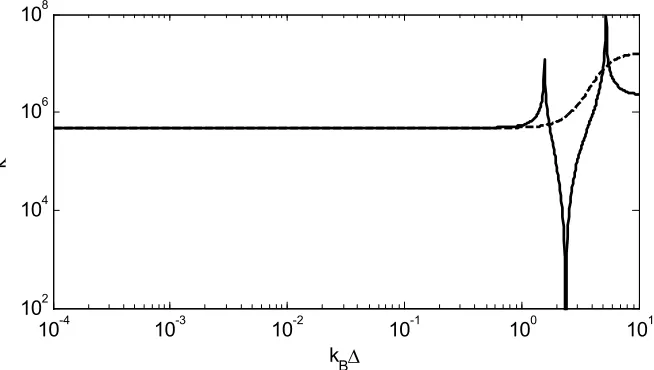
4, which is related to 2

(30)

In this case, the transfer matrix results show marginally better accuracy. This is because the fact that the conditioned eigenvalue problem gives the repeated eigenvalues such that the method is more sensitive to perturbation [24]. For this example, the condition number of the matrices to be inverted in the transfer matrix approach and that in the conditioned eigenvalue problem is about same, as shown in Figure 4.5 (the peaks in the figure correspond to singularities in the matrix to be inverted). In addition, the matrix size is small

(

n=4

)

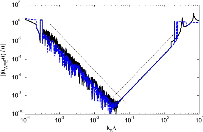
such that the ill-conditioning of the eigenvalue problem is not so significant. Because of these reasons, the transfer matrix approach show better results.

Basically the same discussion holds for the relative errors in the eigenvectors. Figure 4.6 shows the relative errors in the rotational displacement of the eigenvector per unit displacement, which is analytically given by

θ

w =k (e.g. [20,36]). The same trend as the relative error in the wavenumber can be seen.

(31)

10-4 10-3 10-2 10-1 100 101 10-10

10-8 10-6 10-4 10-2 100 102

|(

k

-k B

)

/

k B

|

[image:31.595.116.457.80.302.2]

k_B∆

Figure 4.4: Relative errors in the propagation wavenumber for ― the conditioned eigenvalue problem

(3.9), – – the transfer matrix approach (2.15), ··· asymptote ±40dB decade.

10-4 10-3 10-2 10-1 100 101

102 104 106 108

k B∆

κ

Figure 4.5: The condition numbers of (a) the matrix to be inverted: ― the conditioned eigenvalue

[image:31.595.131.458.396.581.2]

(32)

10-4 10-3 10-2 10-1 100 101 10-10

10-8 10-6 10-4 10-2 100 102

|(θ

W

F

E

-θ

)

/ θ

|

[image:32.595.116.457.80.302.2]

k_B∆

Figure 4.6: Relative errors in the rotational displacement per unit displacement: ― the conditioned

eigenvalue problem (3.9), – – the transfer matrix approach (2.15), ··· asymptote 40dB decade

± .

10-4 10-3 10-2 10-1 100 101

10-10 10-8 10-6 10-4 10-2 100 102

|(

f W

F

E

-f

)

/

f|

[image:32.595.114.460.395.625.2]

k_B∆

Figure 4.7: Relative errors in the shear force per unit displacement. Notation is same as Figure 4.7.

4.3.3 Relative Errors in the Group Velocity

(33)

analytical solution is given by c_g =2

ω

k_B (e.g. [21]). 1000 discretised frequencies are linearly taken in the log space of frequency.

The power and energy relationship and the differentiation of the eigenproblem show accurate results. The differentiation of the eigenproblem is likely to suffer from numerical errors because the method needs D_LR−1 to be evaluated and a large number of matrix operations such that numerical errors may accumulate. Smaller frequency step improves the accuracy of the result using the finite difference method for k_B∆ >0.04 and the error curve follows other two lines, which is the error bound given from the accuracy of the wavenumber.

Regardless of the methods, the numerical results show small errors for the range of, say, 0.01≤ ∆ ≤k_B 1 where both the eigenvalues and eigenvectors are accurately calculated. For the rod case, the range was about 10−6 ≤ ∆ ≤k_L 1. The difference of the lower bound results from the round-off errors due to the inertia term.

10-3 10-2 10-1 100

10-10 10-8 10-6 10-4 10-2 100

k

B∆

|(

c g(W

F

E

)

-c g

/

c g

|

Figure 4.8: Relative errors in the group velocity: ― finite difference, – – power and energy

relationship, −·− differentiation of the eigenproblem.

[image:33.595.96.474.373.607.2]

(34)

5. NUMERICAL EXAMPLE OF A PLATE STRIP

5.1 Introduction

For two-dimensional structures, the conditioned eigenvalue problem should be applied to improve ill-conditioning occurring in the transfer matrix approach. Numerical examples are shown for flexural waves in a thin isotropic plate strip. No damping is assumed.

5.2 Analytical Expression for Flexural Waves in a Plate

A plate strip of width L_y, shown in Figure 5.1, is considered. The plate is thin and isotropic

with simply supported boundary conditions along the y-wise plate edges. For such plate, the analytical wavenumber is given by [36]

2 2 2 x y

h

k k k

D

ρ

ω

= + = ± (5.1)

where D=Eh3 12 1

(

−

ν

2

)

is the bending rigidity, h is the thickness of the plate strip and ν

is the Poisson’s ratio. For the simply supported boundary condition along the plate edges

0, _y

y= L , the wave modes have displacements proportional to sin

(

n y L

π

_y

)

where n is an integer. The wavenumber along the x-direction is then given by

(

)

2 2

1, 2, xn

y

h n

k n

D L

ρ

_ω



π



= ± −_ _ =  

. (5.2)

Substituting k_xn =0 into equation (5.2) gives the cut-off frequency for the nth wave as

(

)

2

1, 2, n

y

D n

n

h L

π

ω

ρ

 

= _ _ =

 

. (5.3)

The group velocity is given from equation (5.2) as

2

gn xn

xn

D

c k

k h

ω

ρ

∂

= =

(35)

[image:35.595.145.421.83.205.2]

Figure 5.1: Simply supported plate strip.

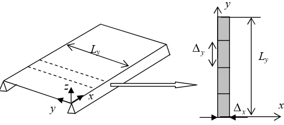
5.3 Flexural Waves in a Plate Strip Using the WFE Method

The flexural waves in the plate strip are solved using the WFE method and results evaluated. In particular, reducing numerical errors is suggested using a FE model with internal nodes.

5.3.1 The WFE Formulation

The plate is assumed to be a steel plate with L_y =0.18, E=2.0 10⋅ 11,

ρ

=7800, ν =0.30 and h=1.8 10⋅ −3, all in SI units. The mass and stiffness matrices are formed using ANSYS 7.1. A four node plane strain shell element (SHELL63), which uses cubic polynomial shape functions for both the x- and y-directions, was chosen. The aspect ratio of FE

γ

= ∆ ∆ ≈_x _y 1 is preferable since k_x∆ ≤_x 1 and k_y∆ ≤_y 1 should be satisfied.

5.3.2 Results Using the Transfer Matrix

The ill-conditioning of the transfer matrix approach is illustrated in this section. Consider a plate strip model comprising 4 elements as shown in Figure 5.2. After removing the in-plane DOFs and DOFs associated with the boundary conditions, there are 22 resulting DOFs for the model. Since the y-wise wavenumber is k_y =n

π

L_y for the nth wave mode, only the n=1 wave mode could be expected to be accurate since k_y∆ =_y

π

4

( )

<1 .

The dispersion relationships are shown in Figures 5.3. The abscissa represents the non-dimensional frequency 2 2

y

L

π

ρ

h D

ω

Ω= and the cut-off frequencies occur at 2

n

Ω = (n=1,2,3…). The ordinate shows the non-dimensional wavenumber, k L_x _y

π

, which becomes

Ly

y

x z

x y

x ∆

Ly y

(36)

-jn for the nth mode at Ω =0 . When k_x∆ =_x 1 then k L_x _y

π

=3.18 , so that the FE discretisation error should be small if k L_x _y

π

<3.18.

The wavenumber calculated from the transfer matrix (2.15) and that from the conditioned eigenvalue problem (3.9) are shown in Figure 5.3 (a) and (b), respectively. There are two waves associated with the n=1 mode. One is a propagating wave which cuts-on at Ω =1 and another is a nearfield wave. In Figure 5.3 (a), it can be seen that the wave near the cut-off frequency

(

Ω =1

)

is inaccurate. This is because the two roots associated with the positive and

negative going wave are such that e±jkx →1 around the cut-off frequency and such roots are likely to be estimated inaccurately because of the ill-conditioning. In turn, relatively accurate results are obtained for the conditioned eigenvalue problem in Figure 5.3 (b) because of the conditioning described in Section 3.

The condition numbers of the matrices to be inverted (D_LR in equation (2.14) and Z₂ in equation (3.9)) and those of the eigenvalue problems (T in equation (2.15) and Z Z₂−1 ₁ in equation (3.9)) are plotted in Figures 5.4. Both the condition number for the matrix to be inverted in Figure 5.4 (a) and that for the eigenvalue problem in Figure 5.4 (b) are worse-conditioned when the transfer matrix approach is used. The condition numbers are almost constant in this frequency range of interest. For plate strip models with more elements, the numerical artefact around the cut-off frequency becomes more prominent because of the worse conditioning and the results using the transfer matrix approach will completely break down.

[image:36.595.154.425.565.613.2]

Figure 5.2: The plate strip FE model, ∆ =_x 18mm,∆ =_y 45mm

(

L_y 4

)

. y

(37)

0.5 1 1.5 2 -5

0 5 10

Ω

Im

(k x L y /π

)

R

e

(k x L y /π

)

0.5 1 1.5 2

-2 -1.5 -1 -0.5 0 0.5 1

Ω

Im

(k x L y

/

π

)

R

e

(k x L y

/

π

)

(a)

(b)

Figures 5.3: Dispersion relationships: ― analytical solution, ···· the WFE result using (a) the transfer

matrix approach, (b) the conditioned eigenvalue problem.

0.5 1 1.5 2

104

105

106

Ω

κ

0.5 1 1.5 2

105

1010

1015

Ω

κ

(a)

(b)

Figures 5.4: The condition numbers of (a) the matrices to be inverted, (b) the eigenvalue problems:

(38)

5.3.3 Relationship between the Condition Number and Matrix

Size

Even for the conditioned eigenvalue problem, the conditioning is still of concern. The condition number κ of the matrix to be inverted is discussed in this section. For flexural waves in a plate strip, the condition number of Z₂ in equation (3.9) is examined. If κ is large, numerical errors occur when the matrix is inverted and the resulting eigenvalue problem is likely to be numerically contaminated.

The condition number depends on the modelling of the plate strip model. Here κ are determined for several plate strip models and the results are shown in Figure 5.5. It can be seen that as (1) ∆_x becomes smaller and (2) the matrix size increases and (3) the aspect ratio γ of the element becomes large, κ increases. From the figure, the relationships between κ, ∆ and the number of elements, N, are approximately expressed as

2 x κ_{∝ ∆}−

or κ∝N2 (5.5)

for the same element aspect ratio. As the number of elements increases, the condition number gets larger because the number of the singular values of the matrix increases which usually results in there being a wider range of the relative magnitudes of the singular values.

Next the effect of the aspect ratio, γ , is determined for the same element area as Figure 5.6. The case of γ =0.2 is also included. For elements of the same area, the dependence in γ is shown in Figure 5.7. The ordinate shows the ratio of κ to that for γ =1. From the figure, the relationships between γ and κ are roughly estimated as

(

)

(

)

2.1 0.4

1 1 , 1 1

γ γ

κ κ

γ

κ κ

γ

−

γ

= ∝ > = ∝ < (5.6)

such that rectangular elements

(

γ

≠1

)

cause κ to be larger. The condition number of the

matrix to be inverted is usually related to

κ

(

D_LR

)

. The matrix D_LR represents the

relationship between forces and displacements across an element, i.e. f_L =D x_LR _R. When the range of the magnitude of elements in D_LR increases, the condition number often

deteriorates. For elements with γ ≠1, only some elements become large compared to others. More detail expression of the effect of γ in D_LR can be seen in [35]. Some elements

(39)

100 101 105

106 107 108 109

∆_x (mm)

κ

a

t Ω

=

7

.4

8

γ=1

γ=2.5

γ=5

γ=0.4

180 150 180

180

90

36

36 75

45

18

12 30

18

Figure 5.5: Condition numbers of the matrix to be inverted at Ω = 7.48 . Each number in the figure

denotes the numbers of elements.

100 101 102

105 106 107 108 109

Area of an element ×10-6 (m2)

κ

a

t

Ω

=

7

.4

8

γ=1

γ=2.5

γ=5

γ=0.4

[image:39.595.136.461.85.350.2]

γ=0.2

[image:39.595.124.453.422.688.2]

On numerical issues for the wave/finite element method

SCIENTIFIC PUBLICATIONS BY THE ISVR

TABLE OF CONTENTS

ABSTRACT

1. INTRODUCTION

1.1 Introduction

1.2 Overview of Periodic Structure Analysis

1.3 Outline of the Report

2. OVERVIEW OF THE WAVEGUIDE FINITE

ELEMENT METHOD

2.1 Introduction

2.2 Finite Element Formulation of a Structural Element

(

)

2.3 Wave Basis

2.3.1 Transfer Matrix

λ

2.3.2 Eigenvalues and Eigenvectors

λ

(

)

(

)

λ

λ

{ }

{

}

2.4 Group Velocity

ω

ω

{ }

{ }

{

}

{

}

{

}

ω

ω

ω

ω

ω

( )

{

(

)

}

( )

λ

ω

ω

ω

( )

( )

( )

( )

3. NUMERICAL ISSUES AND

IMPLEMENTATION

3.1 Introduction

3.2 Conditioning of the Eigenvalue Problem

3.2.1 Mathematical Background of Numerical Errors in the

Eigenvalue Problem

ε κ

( )

ε

( )

κ

( )

κ

( )

κ

( )

( )

( )

λ

( )

( )

( ) ( )