An effective high-order point-collocation numerical approach based on integrated approximants for elliptic differential equations

An effective high-order point-collocation numerical

approach based on integrated approximants for

elliptic differential equations

N. Mai-Duy and T. Tran-Cong

Computational Engineering and Science Research Centre (CESRC)

Faculty of Engineering and Surveying

The University of Southern Queensland, Toowoomba, QLD 4350, Australia

Submitted to

Applied Mathematical Modeling Research Trends,

04-Jun-2007

∗_{Corresponding author: E-mail [email protected], Telephone +61 7 4631 2539, Fax +61 7}

Abstract: This chapter presents the basic features of high-order integral collocation

techniques and demonstrates their application to engineering problems. Emphasis is

placed on the advantage of the integral collocation approach over the conventional

differential approach in the treatment of multiple boundary conditions, complex

geometries and domain decompositions.

Keywords: Radial basis functions, Chebyshev polynomials, Integral collocation

for-mulation, Multiple boundary conditions, Complex geometries, Domain

decomposi-tions.

1

Introduction

Physical phenomena are usually modelled in terms of ordinary differential

equa-tions/partial differential equations (ODEs/PDEs). The DE can only rarely be solved

in an exact manner. As a result, one must resort to numerical techniques to

ob-tain approximate solutions of the DE. The aim of numerical techniques is to reduce

the differential system to an equivalent set of algebraic equations where a solution

becomes obtainable. To achieve that, the field variable and the DE need to be

discretized, relying on the assumption that any continuous quantity can be

approx-imated by a set of continuous functions.

The governing equation can be represented in a strong, weak or inverse form. The

strong form, which is associated with point-collocation techniques such as

finite-difference [1] and pseudospectral [2] methods, does not require the integration of

the DE. The continuous domain is simply replaced by a set of discrete points. The

point-based solution is found using the concept of zero-value of error at certain points

over the domain. On the hand, the weak and inverse forms, which are associated

methods, involve volume and boundary integrals, respectively. The problem domain

or its boundary is divided into a set of small elements. The element-based solution

is determined using the concept of distribution of error within the domain or along

the boundary. Each form has some advantages over the others for certain classes

of problems. The weak and inverse forms possess a smoothing capability, while the

strong form features a mesh-free property.

In a “differential” numerical technique, the field variable approximation is based on

a set of known basis functions with corresponding unknown coefficients.

Expres-sions for its derivatives are then obtained through differentiation. Approximation

schemes can be classified into two categories: low order and high order. Each

cat-egory has its own strengths and weaknesses. The former is straightforward to use.

However, its relative low accuracy requires a very fine structure, which could lead

to numerical difficulty, to represent accurately the complex solution. For the latter,

coarse meshes/grids are usually sufficient for most accuracy requirements. However,

high-order approximation schemes should be used with great care. For instant, the

use of Lagrange polynomials of high order has a tendency to give results that are

oscillatory between data values. Any small level of noise in the interpolating

func-tion will be badly magnified through differentiafunc-tion, causing much larger errors for

its derivative representations.

This chapter reviews a high-order point-collocation numerical approach for elliptic

DEs based on integrated approximants, and associated results recently discussed

in several works, including for example [5-32]. In contrast with the differential

approach described above, Mai-Duy and Tran-Cong [5,8] proposed an integral

pro-cedure, where the starting points of the approximation process are the highest

deriv-atives of the field variable in the given DE. Lower derivderiv-atives, and eventually the

variable itself, are symbolically obtained by integration. These integration processes

therefore facilitate the employment of some extra equations. It is shown that this

feature provides an effective way to handle well-known difficult issues associated

with the differential collocation approach such as [14,15,20,21,27,28,30-32]

• the implementation of multiple boundary conditions,

• the description of non-rectangular boundaries in a Cartesian grid, and

• the imposition of higher-order continuity of the approximate solution across subdomain interfaces.

In addition, the use of integration also improves the quality of the approximation

of derivative functions as well as the stability of a numerical solution owing to its

smoothness property [5-13,16-19,22-26,29].

In this chapter, the integral collocation approach is implemented with radial basis

functions and Chebyshev polynomials. It is noted that other types of basis

func-tions can also be applied. For example, an integrated Sinc function approximation

method has recently been reported by Li and Wu [24]. An attractive feature of

the present high-order integral collocation techniques is that the preprocessing is

simple. The problem domain of regular/irregular shape is discretized by using a

uniform Cartesian grid for radial basis functions and a tensor product grid formed

by Gauss-Lobatto points for Chebyshev polynomials. The approximate expressions

representing the field variable and its derivatives over the domain are constructed

through one-dimensional integrated approximants along grid lines. Superior

accu-racy and convergence of integral collocation techniques over differential collocation

techniques are demonstrated with the solution of differential problems governed

by second- and fourth-order elliptic equations and defined in rectangular and

The remainder of the chapter is organized as follows. Sections 2 and 3 give brief

reviews of high-order approximants and collocation methods, respectively.

Advan-tages of the integral collocation approach are presented in Section 4. Section 5

demonstrates its application to engineering problems including structural analysis

and fluid flow problems. Section 6 concludes the chapter.

2

High-order approximants

2.1

Radial basis function networks (RBFNs)

RBFNs are known as a universal approximator. The RBFN allows the conversion

of a function to be approximated from a low-dimension space to a high-dimension

space in which the function is expressed as a weighted linear combination of RBFs

[33]

f(x) =

m

X

i=1

wigi(x), (1)

where_{gi(x)}m_i=1 the set of RBFs, and {wi}m_i=1 the set of weights to be found.

According to Micchelli’s theorem, there is a large class of RBFs, e.g., multiquadrics,

inverse multiquadrics and Gaussian functions, whose interpolation matrices obtained

from (1) are always invertible provided that the data points are distinct. This is all

that is required for non-singularity of interpolation matrices, whatever the number of

data points and the dimension of problem [34]. It has been proved that RBFNs are

capable of representing any continuous function to a prescribed degree of accuracy

in theLp norm,p∈[1,∞] [35]. On the other hand, according to the Cover theorem,

the higher the number of RBFs used, the more accurate the approximation will be

[36], indicating the property of “mesh convergence” of RBFNs. These important

of ODEs/PDEs.

It has generally been accepted that, among RBFNs, the multiquadric (MQ) scheme

tends to result in the most accurate approximation. The present integral approach

implements the MQ function whose form is

gi(x) =

q

(x₋ci)2+a2i, (2)

where ci and ai are the centre and the width of the ith basis function. The RBF

widths are known to strongly affect the performance of RBFNs. However, there

is still a lack of mathematical theories for specifying their optimal values. For

all numerical examples taken here, the RBF widths are simply chosen as the grid

spacing.

2.2

Truncated Chebyshev series expansions (CSEs)

An approximate function f is sought in the truncated Chebyshev series form [2]

f(x) =

N

X

k=0

akTk(x), (3)

where _{ak}Nk=0 the set of expansion coefficients and {Tk}Nk=0 the set of Chebyshev polynomials of the first kind that are defined by

in which₋1_≤x_≤1. The polynomial Tk(x) can be expanded in power series as

T0(x) = 1 (5)

Tk(x) =

k 2

[_Xk/2]

m=0

(₋1)m2

k−2m_(k−m−1)!

m!(k₋2m)! x

k−2m_{, k > 0 (6)}

where [k/2] is the integer part ofk/2.

The Chebyshev polynomials are orthogonal

Z 1

−1

Tk(x)Tl(x)w(x)dx=

π

2ckδkl, (7)

where w(x) = √1₋x2 _{is the Chebyshev weight function, c}

k = 1 for k ≥ 1 and

ck = 2 for k = 0, and δkl the Kronecker delta.

At the Gauss-Lobatto points xi = cosiπ/N, i = 0, .., N, which are widely used in

collocation methods, the coefficients ak are obtained in an explicit form

ak =

2 N¯ck

N

X

i=0

Tk(xi)

¯ ci

ui, k = 0,1,· · · , N, (8)

where ¯ck = 1 for 1≤k ≤N −1 and ¯ck = 2 for k ={0, N}.

For smooth problems, the Chebyshev approximation scheme exhibits an exponential

3

Methods of collocation

Let Ω be a bounded region and ∂Ω be the boundary of Ω. Consider the differential

problem that consists of an elliptic DE

Lu=b, (9)

and a set of prescribed values along ∂Ω, where _L is some differential operator, b a given function andu the field variable.

Collocation methods are seen to be the simplest way to discretize the DE. It consists

of two main steps. First, the solution u and its derivatives are approximated by

fi-nite sums of smooth functions that are linearly independent. Then, the coefficients

associated with the basis functions are determined by forcing the approximate

so-lution to satisfy the DE and the boundary conditions at certain points (collocation

points). The choice of functions and distribution of collocation points strongly affect

the accuracy of the solution.

This chapter is concerned with two types of very smooth basis functions, namely

radial basis functions (ϕ _≡ g) and Chebyshev polynomials (ϕ _≡ T), that are de-scribed above. In the remainder of the chapter, for consistency of notation between

3.1

Conventional differential formulation

RBFNs/CSEs are employed to represent the variableu, followed by successive

dif-ferentiations to obtain approximate expressions for its derivatives

u(x) =

m

X

i=1

αiϕi(x) = m

X

i=1

αiDi(0)(x), (10)

du(x) dx =

m

X

k=1

αiDi(1)(x), (11)

· · · ·

dp_u(x)

dxp = m

X

k=1

αiDi(p)(x), (12)

whereD(1)_i (x) = dD_i(0)(x)/dx,_{· · ·} , D_i(p)(x) =dD(_ip−1)(x)dx.

It has been proved that there is a reduction in convergence rate for derivative

func-tions and this reduction is an increasing function of derivative order [37,38].

3.2

Present integral formulation

RBFNs/CSEs are employed to represent the highest-order derivatives of the

expressions for its lower-order derivatives and the variable itself

dp_u(x)

dxp = m

X

i=1

αiϕi(x) = m

X

i=1

αiIi(p)(x), (13)

dp−1_u(x) dxp−1 =

m

X

k=1

αiIi(p−1)(x) +c1, (14)

dp−2_u(x) dxp−2 =

m

X

k=1 αiI(p

−2)

i (x) +c1x+c2, (15)

· · · · du(x) dx = m X k=1

αiIi(1)(x) +c1

xp−2

(p₋2)! +c2 xp−3

(p₋3)! +· · ·+cp−2x+cp−1, (16)

u(x) =

m

X

k=1

αiIi(0)(x) +c1

xp−1

(p₋1)! +c2 xp−2

(p₋2)! +· · ·+cp−1x+cp, (17)

where I_i(p−1)(x) = R I_i(p)(x)dx, I_i(p−2)(x) = R I_i(p−1)(x)dx,_{· · ·} , I_i(0)(x) = R I_i(1)(x)dx, and c1, c2,_{· · ·} , cp are integration constants. The integral approximation scheme is

said to be ofpth-order, denoted by ICSE-por IRBFN-p, if thepth-order derivative is

taken as the staring point. The differential approximation scheme can be considered

as a special case of the integral approximation scheme by setting the value of p to

zero.

The evaluation of (13)-(17) at a set of collocation points _{xi}m_i=1 leads to

d

dp_u

dxp =Ib

(p)

[p]bs, (18)

d

dp−1_u dxp−1 =Ib

(p−1)

[p] bs, (19)

· · · ·

c

du dx =Ib

(1)

[p]bs, (20)

u=_Ib_[(0)_p]bs, (21)

and derivative function, respectively,

b

s= (α1, α2,_{· · ·} , αm, c1, c2,· · · , cp)T ,

b

I[(pp])=

        

I1(p)(x1), I (p)

2 (x1), · · · , I (p)

m (x1), 0, 0, · · · , 0, 0

I₁(p)(x2), I2(p)(x2), · · · , Im(p)(x2), 0, 0, · · · , 0, 0

· · · ·

I₁(p)(xm), I2(p)(xm), · · · , Im(p)(xm), 0, 0, · · · , 0, 0

         , b

I[(pp]−1) =

        

I1(p−1)(x1), I (p−1)

2 (x1), · · · , I (p−1)

m (x1), 1, 0, · · · , 0, 0

I₁(p−1)(x2), I(p

−1)

2 (x2), · · · , I(p

−1)

m (x2), 1, 0, · · · , 0, 0

· · · ·

I₁(p−1)(xm), I2(p−1)(xm), · · · , Im(p−1)(xm), 1, 0, · · · , 0, 0

         ,

· · · ·, and

b

I[(0)p] =

        

I₁(0)(x1), I₂(0)(x1), _{· · ·} , Im(0)(x1), x

p−1 1

(p−1)!,

xp₁−2

(p−2)!, · · · , x1, 1 I1(0)(x2), I

(0)

2 (x2), · · · , I (0)

m (x2), x

p−1 2

(p−1)!,

xp₂−2

(p−2)!, · · · , x2, 1

· · · ·

I₁(0)(xm), I2(0)(xm), · · · , Im(0)(xm), x

p−1

m (p−1)!,

xpm−2

(p−2)!, · · · , xm, 1

         .

The use of integrated basis functions is expected to overcome the problem of

reduc-tion of convergence rate caused by differentiareduc-tion. Numerical studies on second-order

differential problems [5,18,19,29] have indicated that the integral approach produces

more accurate results than the differential one. This has recently been theoretically

examined with RBFs by Sarra [22], which show the superiority in accuracy of the

antiderivative approach.

Another important point here is that additional coefficients (integration constants)

can be utilized to handle “extra constraints” related to boundary conditions and

4

Advantages of the integral collocation approach

4.1

Treatment of multiple boundary conditions

For simplicity, consider the approximation of the solution of the biharmonic equation

∂4_u ∂x4 + 2

∂4_u ∂x2_∂y2 +

∂4_u

∂y4 =b(x, y), (22)

in a rectangular domain with double boundary conditionsu and ∂u/∂n.

For the differential collocation approach, there is normally one equation employed at

a point. Boundary conditions for second-order equations (single boundary values)

can thus be accommodated in a straightforward manner. However, for higher-order

equations, the solution is required to satisfy more than one prescribed value at a

boundary point. A number of techniques have been developed for handling

multi-ple boundary conditions, including (i) the node-reduction technique (reducing the

number of collocation points used for collocating the governing equation), (ii) the

fictitious-point technique (using fictitious points as additional unknowns), and (iii)

the imposed-kernel technique (modifying the basis functions to incorporate

bound-ary conditions). In contrast, the integral collocation approach has the ability to

deal with multiple boundary conditions in a natural way. The presence of

integra-tion constants allows the use of more than one equaintegra-tion at certain points. Such

extra equations can be utilized for the purpose of imposing the value of the normal

derivative and the governing equation at boundary points.

In currently used notations, _b and _e denote vectors/matrices that are associated with a grid line (one-dimensional domain) and the whole set of grid lines

The integral collocation schemes of fourth order are employed here to discretize

derivative terms in the biharmonic equation. It is more convenient to work in the

physical space than in the spectral space. Consider a horizontal grid line. The

presence of four integration constants in the integral formulation allows one to add

four extra equations to the conversion system. These equations can be chosen to

represent the value of the normal derivative and the governing equation at both ends

of the line. The conversion process of the spectral space into the physical space is

constructed by _

  bu

b v   =    Ib

(0) [4] b B       αb

b

c

  =_Cb

   αb

b

c

 

, (23)

where_Ib_[4](0) is defined as before,

b α=          α1 α2 · · ·

αnx

        

, bc=

         c1 c2 c3 c4         

, bu=

         u1 u2 · · ·

unx

         , b v =          ∂u ∂x(x1) ∂u ∂x(xnx) b(x1)₋2_∂x∂42u_y2(x1)−

∂4_u

∂y4(x1)

b(xnx)−2

∂4_u

∂x2_y2(xnx)−

∂4_u

∂y4(xnx)

         , b B=         

I₁(1)(x1) · · · In(1)x(x1) x 2

1/2 x1 1 0 I₁(1)(xnx) · · · I

(1)

nx(xnx) x 2

nx/2 xnx 1 0 I₁(4)(x1) _{· · ·} In(4)x(x1) 0 0 0 0 I₁(4)(xnx) · · · I

(4)

nx(xnx) 0 0 0 0

         [4] ,

Solving (23) yields _

  αb

bc

  =_Cb−1

   ub

b

v

 

. (24)

Taking (24) into account, the values of derivatives of the variable u at a point on

the line are computed by

∂4_u(x) ∂x4 =

I₁(4)(x), I₂(4)(x),_{· · ·} , I_n(4)_x(x),0,0,0,0_Cb−1

   ub

b

v

 

, (25)

∂3_u(x) ∂x3 =

I₁(3)(x), I₂(3)(x),_{· · ·} , I_n(3)_x(x),1,0,0,0_Cb−1

   ub

b

v

 

, (26)

∂2_u(x) ∂x2 =

I₁(2)(x), I₂(2)(x),_{· · ·} , I_n(2)_x(x), x,1,0,0_Cb−1

   ub

b

v

 

, (27)

∂u(x) ∂x =

I₁(1)(x), I₂(1)(x),_{· · ·} , I_n(1)_x(x),x 2

2, x,1,0

b

C−1

   ub

b

v

 

. (28)

The evaluation of (25)-(28) at the grid points leads to

d_∂i_u

∂xi =Dbix

   bu

b

v

 

, i=_{1,2,3,4_}, (29)

where c∂_∂xiui =

∂i_u

1

∂xi ,

∂i_u

2

∂xi ,· · · ,

∂i_u nx

∂xi

T

and _Dbix is the nx×(nx+ 4) matrix of known

quantities related to geometry and discretization.

Expression (29) can be rewritten as c∂_∂xiui = Db

†

ixub+Db

‡

ixbv, where Db

†

ix and Db

‡

ix are

matrices that are formed by the first nx columns and the last four columns of the

matrix _Dbix, respectively. The extra information vector bv (components v3 and v4)

contains some unknown values—the mixed partial derivative∂4_u/∂x2_∂y2 _{at the two}

combinations of nodal values of the variableu(the detailed expression of∂4_u/∂x2_∂y2

will be given later on). As a result, one can express (29) in terms of nodal variable

values only. The values of the ith-order derivative of u with respect to y at the

collocation points along a vertical line will be obtained in the same way.

The approximations for derivatives over 2D grids can be conveniently constructed by

means of Kronecker tensor products. Assuming that the grid points are numbered

from bottom to top and from left to right, the values of derivatives of u at the grid

points are computed by

g

∂i_u

∂xi =

b

Dix⊗Iby

e

u+ekix,

g_∂i_u

∂yi =

b

Ix⊗Dbiy

e

u+ekiy, (30)

where_⊗is the Kronecker tensor product,_IbxandIby are the identity matrices of sizes

nx ×nx and ny ×ny, respectively, ekix and ekiy are the vectors of known quantities

related to boundary conditions, and _eu= u1, u2,_{· · ·} , unxny

T

.

The integral collocation approach employs the following relation to calculate the

mixed fourth-order derivative

∂4_u ∂2_x∂2_y =

1 2

∂2 ∂x2

∂2_u ∂y2

+ ∂ 2

∂y2

∂2_u ∂x2

. (31)

This expression reduces the computation of fourth-order mixed derivatives to that

of second-order pure derivatives for which IRBFNs/ICSEs involve integration with

respect toxoryonly. Integral schemes of second order are used here to approximate

these second-order derivatives with the extra information being the values of the

corresponding first-order derivatives at the boundary points.

It can be seen that the integrated approximants contain information about boundary

conditions. As a result, it remains only to force these approximations to satisfy the

determinate system of algebraic equations for the unknown vector of nodal interior

values of the variableu.

The integral and differential collocation approaches are applied to solve the following

test problem

b(x, y) = 4 sin(πx) sin(πy), (32)

ue =

1

π4 sin(πx) sin(πy), (33) Ω_≡[₋1,₋1]_×[1,1], (34)

whereue denotes the exact solution of the problem.

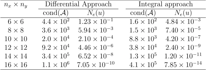
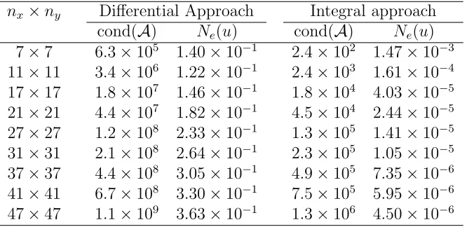
Results concerning the discrete relative L2 error of the solution u, Ne(u), and the

condition number of the system matrix, cond(_A), obtained by the two approaches are presented in Tables 1 and 2 for CSEs and RBFNs, respectively. For the

differ-ential approach, double boundary conditions are implemented here using the

node-reduction technique. The PDE is collocated at the (nx−4)(ny −4) interior points

(xi, yj), i = (3,4,· · · , nx −2), j = (3,4,· · ·, ny −2). Along the two vertical lines,

boundary conditions ∂u/∂nare imposed at the 2(ny−2) nodal points; while along

the two horizontal lines, they are imposed at the 2(nx−4) nodal points. The

dis-cretized boundaries do not include the four corners of the domain. This leads to a

square set of algebraic equations. Like conventional RBF techniques, the present

differential RBF collocation technique approximates a solution in terms of network

weights. For both cases (RBFNs and CSEs), the performance of the integral

4.2

Description of non-rectangular boundaries in a

Carte-sian grid

The application of finite-difference and pseudospectral methods to irregularly-shaped

domains requires coordinate transformations. First, a physical domain of complex

geometry is converted into a computational domain of regular geometry. Then, an

equivalent problem is derived by transforming the governing equation into the

com-putational coordinate system. The relationships between the two coordinates

sys-tems are usually given in the form of PDEs. Such a procedure is quite cumbersome.

In contrast, the complicated coordinate transformations are avoided in

Cartesian-grid methods, which are the concern of this section. They are implemented with

ICSEs and IRBFNs. The incorporation of prescribed values on immersed

bound-aries are conducted in a way that does not adversely affect the accuracy of the

numerical method. There are some differences in boundary treatment between the

two present approximation schemes, which are presented through the second-order

Dirichlet differential problem governed by

∂2_u ∂x2 +

∂2_u

∂y2 =b(x, y), (35)

in a circular domain Ω with a unit radius.

4.2.1 ICSEs

Figure 1 shows an extension of Ω to the reference square that is discretized using

a tensor product grid formed by Gauss-Lobatto points. It can be seen that the

grid points do not generally lie on the boundary of the domain. Integration

con-stants are utilized here to include information on the boundary in the Chebyshev

Lines aa′ _{and bb}′ _{in Figure 1 present typical cases for the approximation of ∂u/∂x}

and ∂2_u/∂x2_.

4.2.2 Case 1 - Line aa′_:

Along this line, there are two boundary points xb1 and xb2. Assume that they are

not grid points. The ICSE-2 scheme can be employed to impose the two boundary

conditions. The conversion of the spectral space into the physical space is based on

the following system

      b u

ub1

ub2

     =    Ib

(0) [2] b B          b α c1 c2      = b C       b α c1 c2     

, (36)

where_Ib_[2](0) is as before,

b

α= (α1, α2,_{· · ·} , αnx)T , (37)

b

u= (u1, u2,· · · , unx)

T , (38) b B=    I (0)

1 (xb1), I2(0)(xb1), · · ·, In(0)x(xb1), xb1, 1 I₁(0)(xb2), I2(0)(xb2), · · ·, In(0)x(xb2), xb2, 1

  

[2] ,

and nx is the number of collocation points on the grid line.

Solving (36) yields _

     b α c1 c2      = b

C−1

      b u

ub1

ub2

    

The values of∂u/∂x and ∂2_u/∂x2 _{at the grid points are then computed by}

c

∂u ∂x =Ib

(1) [2]Cb

−1       b u

ub1

ub2

    

, (40)

d

∂2_u ∂x2 =Ib

(2) [2]Cb

−1       b u

ub1

ub2

    

. (41)

4.2.3 Case 2 - Line bb′_:

A number of schemes can be applied here. In the following, two typical schemes are

presented.

If the contact pointxb is not a grid node, one can use ICSE-1

   ub

ub   =    Ib

(0) [1] b B       αb

c1

 

, (42)

where

b

B=

I₁(0)(xb), I2(0)(xb), · · ·, In(0)x(xb), 1

[1] .

If the contact point is also a grid node, one can employ ICSE-0 or ICSE-2. For the

latter, the conversion system is given by

      b u ∂ub ∂x

∂2_u

b ∂x2      =    b

I[2](0)

b B          b α c1 c2     

where

b

B =

   I

(1)

1 (xb), I2(1)(xb), · · · , In(1)x(xb), 1, 0 I₁(2)(xb), I2(2)(xb), · · · , In(2)x(xb), 0, 0

  

[2] .

In (43),∂ub/∂xand∂2ub/∂x2are known values, which are derived from using

bound-ary conditions.

The remaining steps for obtaining the Chebyshev approximations of ∂u/∂x and

∂2_u/∂x2 _{are similar to Case 1 and therefore omitted here for brevity.}

The values of ∂u/∂y and ∂2_u/∂y2 _{at the grid points along vertical lines can be}

computed in a similar fashion.

The Chebyshev approximations of derivatives at a grid point are expressed in terms

of the nodal values ofualong the grid lines that goes through that point. It should

be emphasized that they already contain information about the boundary of Ω

(i.e. locations and boundary values). As with finite-difference, finite-element and

boundary-element techniques, one will gather these approximations together to form

the global matrices for the discretization of the PDE. This task is relatively simple

since the grid used here is regular. By collocating the governing equation at the grid

points and then deleting rows corresponding to points that lie on the boundary, a

square system of algebraic equations is obtained, which is solved for the approximate

solution.

4.2.4 IRBFNs

Unlike ICSEs, IRBFNs have the capability to handle unstructured points with

ac-curacy. The problem domain is embedded in a Cartesian grid with a grid spacing

h. Grid points outside the domain (external points) together with internal points

remaining grid points are taken to be the interior nodes (Figure 2). The boundary

nodes consists of the grid points that lie on the boundaries, and points that are

generated by the intersection of the grid lines with the boundaries.

The one-dimensional IRBFN schemes are employed to discretize the solution and

its relevant derivatives along grid lines. As presented earlier, an IRBFN-p scheme

permits the approximation of a function and its derivatives of orders up to p. To

use integrated basis functions only, one needs to employ IRBFNs of at least second

order. A line in the grid contains two sets of points (Figure 3). The first set consists

of the interior points that are also the grid nodes (regular nodes). The values of

the variable u at the interior points are unknown. The second set is formed from

the boundary nodes that do not generally coincide with the grid nodes (irregular

nodes). At the boundary nodes, the values of the variableuare given. Unlike

finite-difference and pseudospectral methods, the involvement of irregular points here does

not adversely affect the accuracy of the IRBFN scheme.

Consider a horizontal grid line (Figure 3). An important feature of the present

IRBFN technique is that, along the grid line, both interior points_{xi}q_i=1 and

bound-ary points _{xbi}2_i=1 are taken to be the centres of the network. This work employs

IRBFN-2s to discretize the field variable. The conversion system is constructed as

follows _      b u

ub1

ub2

     =    b

I[2](0)

b B          b α c1 c2      = b C       b α c1 c2     

where_Ib_[2](0) is defined as before,

b

u= (u1, u2,· · · , uq)T ,

b

α = (α1, α2,_{· · ·} , αm)T ,

b B =    I (0)

1 (xb1) · · · Im(0)(xb1) xb1 1 I₁(0)(xb2) · · · Im(0)(xb2) xb2 1

  

[2] ,

and m=q+ 2.

The obtained system (44) for the unknown vector of network weights can be solved

using the singular value decomposition technique

      b α c1 c2      = b

C−1

      b u

ub1

ub2

    

. (45)

The values of the first and second derivatives ofuat the interior points are computed

as follows          ∂u1 ∂x ∂u2 ∂x ... ∂uq ∂x          =         

I₁(1)(x1) _{· · ·} Im(1)(x1) 1 0

I1(1)(x2) · · · I (1)

m (x2) 1 0

· · · ·

I₁(1)(xq) · · · Im(1)(xq) 1 0

         [2] b

C−1

      b u

ub1

ub2

    

, (46)

and _        

∂2_u 1

∂x2

∂2_u 2

∂x2

...

∂2_uq

∂x2          =         

I₁(2)(x1) _{· · ·} Im(2)(x1) 0 0

I₁(2)(x2) _{· · ·} Im(2)(x2) 0 0

· · · ·

I1(2)(xq) · · · Im(2)(xq) 0 0

         [2] b

C−1

      b u

ub1

ub2

    

or in compact forms

c

∂u

∂x =Db1xub+bk1x, (48) and

d

∂2_u

∂x2 =Db2xbu+bk2x, (49) wherebk1xandbk2xare the vectors of known quantities related to boundary conditions.

It can be seen from (48) and (49) that the IRBFN approximations of ∂u/∂x and

∂2_u/∂x2 _{at the interior points include information about the boundary (locations}

and boundary values).

The incorporation of the boundary points into the set of centres has several

advan-tages:

• It allows the two sets of centres and collocation points to be the same, i.e.

{ci}mi=1 ≡

{xi}qi=1∪ {xbi}2i=1 . Numerical investigations have indicated that when these two sets coincide, the RBF approximation scheme tends to result

in the most accurate numerical solution [5,6].

• It allows the use of IRBFNs with a fixed order (IRBFN-2), regardless of the shape of the domain. In contrast, the order of the ICSE scheme depends on

the number of intersections between a grid line and the boundaries.

In the same manner, one can obtain the IRBF expressions for∂u/∂y and ∂2_u/∂y2

at the interior points along a vertical line.

The “local” IRBF approximations along grid lines will be assembled to build the

discrete representation of the PDE. Collocating the governing equation at the

inte-rior points results in a square system of algebraic equations, which is solved for the

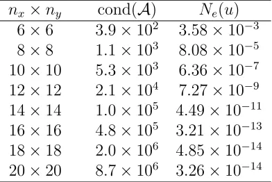
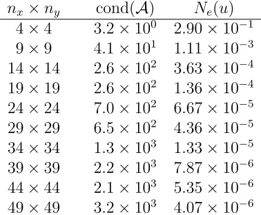
Numerical studies are conducted for the following driving and exact functions

b(x, y) = ₋2 sin(πx) sin(πy), (50) ue(x, y) =

1

π2 sin(πx) sin(πy). (51)

Condition numbers of the system matrix and relative L2 errors of the solution u

are shown in Tables 3 and 4 for ICSEs and IRBFNs, respectively. Results indicate

that the two techniques preserve their fast rates of convergence with grid refinement.

The process of handling irregular geometries here is much simpler than that using

coordinate transformations.

4.3

Improvement of continuity order across subdomain

in-terfaces

The use of domain decompositions (DDs) is necessary to handle large-scale domains

and complex geometries. The problem domain is partitioned into a set of

subdo-mains that can be overlapped or non-overlapped. An important feature of DDs is

that the size of the matrices involved is much smaller than that associated with a

single domain. With the recent emergence of parallel computers, the DD methods

have become more attractive because they allow the parallel implementation of

dis-cretization schemes. However, the main drawback of the DD methods is that they

provide a less smooth solution than a single-domain method. Let p be the order

of the governing equation. Conventional DD techniques are only able to impose a

C(p−1) _{solution across subdomain interfaces, a situation we seek to improve here.}

This chapter is concerned with non-overlapping domain decompositions. It is shown

that the integral collocation approach has the capability to force the Cp_{, instead}

interfaces.

For the sake of simplicity, the basic features of the present DD scheme are described

through the following second-order ODE

κd 2_u

dx2 +β du

dx +γu=b(x), (52)

defined on the domain a_≤ x_≤b and subject to the Dirichlet boundary conditions at both ends: ¯ua and ¯ub.

A substructuring method [39] is applied here, which involves two main steps: (i)

To find the values of the variableuat the interface points/interior-boundary-points

(the interface solution) and (ii) To find the values of the variable u at the interior

points in subdomains (the subdomain solution). The present substructuring

tech-nique is based on the use of integrated approximants (ICSEs/IRBFNs) to represent

approximate solutions in subdomains.

4.3.1 The interface solution

The domain of interest is divided intoM subdomains. Each subdomain is discretized

using a set of n Gauss-Lobatto points via the following coordinate transformation

x[j] = x [j]

r −x[_lj]

2 ξ+

x[rj]+x[_lj]

2 = L[j]

2 ξ+

x[rj]+x[_lj]

2 , (53)

in which x[_lj] and x[rj] are the coordinates of the boundary points of a subdomain j,

L[j]_=x[j]

The continuity of the solution and its flux leads to the following constraint equations

u[_nj] = u[₁j+1], (54)

du dx

[j]

n

=

du dx

[j+1] 1

, (55)

wherej =_{1,2,_{· · ·} , M ₋1_}.

The present scheme requires the solutionu to be continuous, i.e.

u[_nj] =u[₁j+1]= ¯uj, j ={1,2,· · · , M−1}, (56)

and its derivatives to be matched at the interfaces. This approach allows an easy

implementation (automation) of the computer code.

Consider a subdomainj. Using integrated approximations (13)-(17) withp= 2, the

governing equation (52) and the boundary conditions can be transformed into

4κ L[j]2

n

X

k=1

α[_kj]I_k(2)(ξ) + 2β L[j]

n

X

k=1

α[_kj]I_k(1)(ξ) +c[₁j]

!

+γ

n

X

k=1

α_k[j]I_k(0)(ξ) +c₁[j]ξ+c[₂j]

!

=b(x[j](ξ)), (57)

n

X

k=1

α_k[j]I_k(0)(₋1)₋c₁[j]+c[₂j]= ¯uj−1, (58)

n

X

k=1

α_k[j]I_k(0)(+1) +c₁[j]+c[₂j]= ¯uj, (59)

where ¯uj−1 = ¯ua for j = 1, ¯uj = ¯ub for j = M, and the unknowns are the set of

expansion coefficients and integration constants.

form

A[j]

               

α[₁j]

α[₂j]

· · ·

α[nj]

c[₁j]

c[₂j]

                =                

b[₁j]

b[₂j]

· · ·

b[nj]

¯ uj−1

¯ uj                 , (60) or

A[j]bs[j] =

     

bb[j] ¯ uj−1

¯ uj     

, (61)

whereA[j]_{is the known matrix of dimension (n+ 2)×(n+ 2). Unlike conventional} differential formulations, the governing equation (52) is forced to be satisfied at the

two boundary points exactly in (61) (the first andnth rows)

κ

d2_u dx2

[j] 1

+β

du dx

[j] 1

+γu[₁j] = b[₁j], (62)

κ

d2_u dx2

[j]

n

+β

du dx

[j]

n

+γu[j]

n = b[nj]. (63)

Solving (61) yields

b

s[j]= A[j]−1

     

bb[j] ¯ uj−1

¯ uj     

. (64)

As mentioned earlier, the interface unknown vector, namely (¯u1,u2,¯ _{· · ·} ,u¯M−1)T, are

the interfaces du dx [1] n = du dx [2] 1 , (65) du dx [2] n = du dx [3] 1 , (66) · · · · du dx

[M−1]

n

=

du dx

[M] 1

, (67)

where

du[j]_(x(ξ))

dx =

2 L[j]

n

X

k=1

α_k[j]I_k(1)(ξ) +c[₁j]+ 0

!

= 2 L[j]

h

I₁(1), I₂(1),_{· · ·} , I_n(1),1,0i_bs[j]. (68)

Substituting (64) into (65)-(67) and then imposing the prescribed boundary

condi-tions ¯ua and ¯ub yield the following square system of equations

Af          ¯ u1 ¯ u2 · · · ¯ uM−1

        

=bg, (69)

whereAf is the known interface matrix of dimension (M−1)×(M−1), andbg the

vector of known quantities related tob(x), ¯ua and ¯ub.

imposed at an interfacej

u[_nj]=u[₁j+1], (70)

du dx

[j]

n

=

du dx

[j+1] 1

, (71)

κ

d2_u dx2

[j]

n

+β

du dx

[j]

n

+γu[_nj]=b[_nj], (72)

κ

d2_u dx2

[j+1] 1

+β

du dx

[j+1] 1

+γu[₁j+1]=b[₁j+1]. (73)

Sinceb[nj]=b[1j+1], (70)-(73) lead to

d2_u dx2

[j]

n

=

d2_u dx2

[j+1] 1

. (74)

Thus,Cp _{continuity (p= 2 in this example) is automatically satisfied in general.}

4.3.2 The subdomain solution

Substitutions of the interface values obtained from solving (69) into (64) yield the

sets of expansion coefficients and integration constants for subdomains, and hence

the solution to the original problem is obtained. It is noted that each subdomain

can be analyzed separately, offering an opportunity for parallelization.

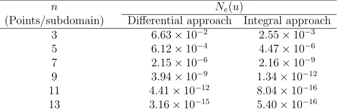
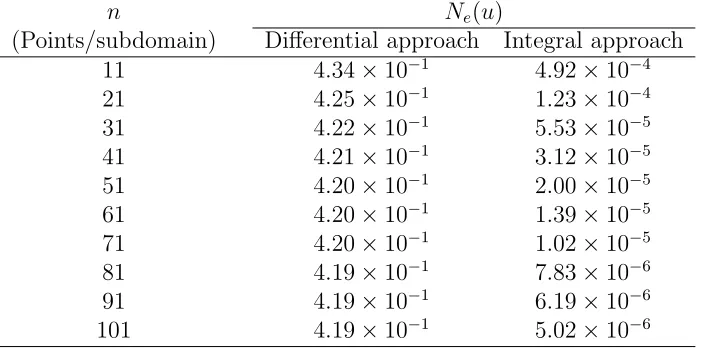
Numerical results are presented for the following data

κ = 1, β = 0, γ = 0, (75)

b =₋sin(πx), (76) ue =

1

π2 sin(πx), (77)

The problem domain is decomposed into 5 subdomains of equal length. Each

sub-domain is discretized using different sets of collocation points. The accuracy of a

numerical technique is presented in the form of the relativeL2norm of the solutionu

calculated at a test set of 201 uniformly distributed points. Both CSEs and RBFNs

are applied here. Parameters used in the differential and integral approaches are

exactly the same (e.g. RBF widths are all chosen as grid spacing). Tables 5 and 6

indicate that the DD scheme based on integration performs much better than that

based on differentiation.

The present numerical schemes can be extended to solve higher-dimensional

prob-lems and higher-order DEs. Similarly, the Cp _{continuity of the solution over}

con-tiguous regions is achieved owing to the satisfaction of the governing equation at the

boundary points in each subdomain. The boundary conditions at the interfaces can

be chosen to be_{u, du/dn, ..., dp/2−1_u/dnp/2−1_{}, and these unknown values are then} determined by the imposition of continuity in the (p/2),(p/2+1),_{· · ·} ,(p₋1)th-order normal derivatives across the interfaces.

5

Some applications of the integral collocation

approach

This section presents several applications of the integral collocation approach in

the simulation of engineering problems. The first two problems are concerned with

5.1

Free vibration of ring-like structures

The structural element is a ring of rectangular cross-section of constant width and

thickness that varies parabolically according to the relation (Figure 4):

h(¯θ) = h(0)

− 4

π2(r−1)¯θ 2₊ 4

π(r−1)¯θ+ 1

=h(0)f(¯θ), (79)

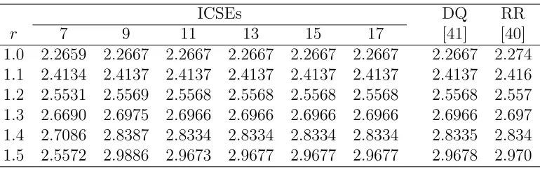
where r = h(π/2)/h(0). The case of normal, in-plane modes of vibration is

con-sidered here, where only flexural effects are taken into account and one disregards

stretching in the axial direction. Its vibrational behaviour can be modelled by a

sixth-order ODE. The problem is simulated with ICSEs. The obtained results are

compared with those of the optimized Rayleigh-Ritz method [40] and the differential

quadrature technique [41].

5.1.1 A circular ring with supports

Since the structure is symmetric, only half of the domain is considered.

Introduc-ing the dimensionless variable θ = ¯θ/π, the governing differential equation can be

expressed in the form

β1v[6]+β2v[5] +β3v[4] +β4v′′′ +β5v′′+β6v′ ₋Ω2f v′′+f′v′ ₋π2f v= 0, (80)

with boundary conditions

where v[q] _{= d}q_v/dθq_{, v is the tangential displacement, θ is the dimensionless}

vari-able, Ω is the dimensionless frequency, and

0_≤θ_≤1,

β1 =φ/π4, β2 = 3φ′/π4, β3 = (2φ/π2) + (3φ′′/π4),

β4 = (4φ′/π2) + (φ′′′/π4), β5 =φ+ (3φ′′/π2), β6 =φ′ + (φ′′′/π2),

φ= [f(θ)]3, f(θ) = ₋4(r₋1)θ2+ 4(r₋1)θ+ 1.

The variable coefficients in (80) involve sixth-order polynomials in θ. Six data

sets, _{7,9,_{· · ·} ,17_} Gauss-Lobatto points, are employed to study the convergence behaviour of the present method. Results concerning the fundamental frequency

coefficient are shown in Table 7. They are compared well with those of [40] and [41].

It can be seen that the present method achieves a high level of accuracy using only

a few grid points. For r = 1.5, at least 4 significant digits remain constant when

n_≥13.

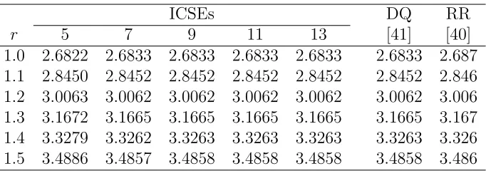
5.1.2 A completely-free ring

In this case, a quarter of the ring structure is considered. It is convenient to introduce

the dimensionless variable θ = ¯θ/(π/2) here and the governing equation can be

written as

β1v[6]+β2v[5]+β3v[4]+β4v′′′+β5v′′+β6v′₋Ω2f v′′+f′v′₋π2f v/4= 0, (81)

with boundary conditions

where

0_≤θ_≤1,

β1 = 16φ/π4, β2 = 48φ′/π4, β3 = (8φ/π2) + (48φ′′/π4),

β4 = (16φ′/π2) + (16φ′′′/π4), β5 =φ+ (12φ′′/π2), β6 =φ′ + (4φ′′′/π2),

φ= [f(θ)]3, f(θ) = ₋(r₋1)θ2+ 2(r₋1)θ+ 1.

Convergence studies are conducted using five data sets of _{5,7,_{· · ·} ,13_} Gauss-Lobatto points. Table 8 shows the fundamental frequencies obtained by the present

method together with those of [40] and [41]. It can be seen that they are in good

agreement. Highly accurate results are obtained with the present technique. For

r= 1.5, at least 4 significant digits remain constant when n_≥9.

5.2

Laminated composite plate

Laminated fibre composite plates have been extensively used in many fields of

en-gineering such as aeronautics and space industries. Much research effort has been

dedicated to improve the ability to predict the behaviour of these structures.

Using the first-order shear deformation theory, the equilibrium equations for

moderately-thick laminated composite plates without membrane action can be written in the

form [42]

A45 ∂ 2_w

∂x∂y − ∂ψy

∂x

+A55 ∂ 2_w

∂x2 + ∂ψx

∂x

+A44 ∂ 2_w

∂y2 − ∂ψy

∂y

+A45 ∂ 2_w

∂x∂y + ∂ψx

∂y

D16 ₋∂ 2_ψ

x

∂x2

+D26 ₋ ∂ 2_ψ

y

∂x∂y

+D66 ∂ 2_ψ

x

∂x∂y − ∂2_ψ

y

∂x2

+

D12 ₋ ∂ 2_ψ

x

∂x∂y

+D22 ₋ ∂ 2_ψ

y

∂y2

+D26 ∂ 2_ψ

x

∂y2 − ∂2_ψ

y

∂x∂y

=A44 ∂w ∂y −ψy

+A45 ∂w ∂x +ψx

, (83)

D16 ₋ ∂ 2_ψ

x

∂x∂y

+D26 ₋ ∂ 2_ψ

y

∂y2

+D66 ∂ 2_ψ

x

∂y2 − ∂2_ψ

y

∂x∂y

+

D11 ₋ ∂ 2_ψ

x

∂x2

+D12 ₋ ∂ 2_ψ

y

∂y∂x

+D16 ∂ 2_ψ

x

∂y∂x− ∂2_ψ

y

∂x2

=A45 ∂w ∂y −ψy

+A55 ∂w ∂x +ψx

, (84)

wherew is the transverse displacement of a point situated in the middle plane, the

xy plane; ψx and ψy are respectively the rotations of the transverse normal, i.e. in

the z direction, with respect to the y and x axes;q(x, y) is the transverse load; and

Dij =

1 3

n

X

k=1

(h3_k−h3_k−1)(Qij)(k) i, j = 1,2,6, (85)

Aij =κ n

X

k=1

(hk−hk−1)(Cij)(k), (86)

in whichκ= 5/6 is a shear correction factor, his the thickness of the laminate, and

Qij andCij represent the stiffness constants of a unidirectional orthotropic composite

making an angleθ with the principal material x-axis. Equations (82)-(84) involve a

large number of derivative terms, some of which are mixed partial derivatives.

The IRBFN method is applied to the static analysis of the bending behaviour of

a simply-supported cross-ply laminate a_×a with a cut-out concentric square hole a/2_×a/2. The composite plate consists of four layers 00_/900_/900_/00 _{under a uniform} pressureq0. The material properties are chosen to be

E1 = 25E2, ν12 = 0.25,

Different grids are employed for the study of grid convergence. A typical grid is

plotted in Figure 5. Results are presented in dimensionless forms according to the

following relations

w_→ 100E2h 3

q0a4 w, (87)

{σxx, σyy, τxy} →

h2 q0a2{

σxx, σyy, τxy}, (88)

{τyz, τxz} →

h

q0a{τyz, τxz}. (89)

Good convergence is achieved as shown in Table 9. Figure 6 shows distributions of

the displacement and in-plane stresses calculated atz =h/2.

5.3

Driven-cavity viscous flow

This problem is usually used as a model for the understanding of physical flows and

for the testing of new numerical schemes in CFD. The lid-driven cavity flow possesses

physically unrealistic characteristics (discontinuous velocity) at the edges of the lid.

This leads to a rapid change in stress near those points, thereby making the

nu-merical simulation difficult. In the context of Newtonian-fluid flow, Ghia, Ghia and

Shin [43] have reported accurate solutions for a wide range of the Reynolds number

using a multigrid finite-difference scheme with very dense grids. These results have

often been cited in the literature for comparison purposes. Recently, by using the

Chebyshev collocation technique, which exhibits exponential convergence/spectral

accuracy, for the calculation of a regular part of the solution, and by using analytical

formulae to obtain the singular part, Botella and Peyret [44] have provided

bench-mark spectral results on the flow at Re = 1000. It will be shown that the IRBFN

results are in closer agreement with the spectral solutions than the finite-difference

The lid velocity (U) and the side length of the cavity (L) are used as reference

quantities. The dimensionless governing equations for unsteady two-dimensional

incompressible flow of a Newtonian fluid in terms of stream functionψ and vorticity

ω can be written as follows

∂ω ∂t +

∂ψ ∂y

∂ω ∂x −

∂ψ ∂x

∂ω ∂y

= 1 Re

∂2_ω ∂x2 +

∂2_ω ∂y2

, (90)

∂2_ψ ∂x2 +

∂2_ψ

∂y2 =−ω, (91)

whereRe=U L/νis the Reynolds number(ν: the kinematic viscosity). The vorticity

and stream function are defined by

ω = ∂v ∂x −

∂u

∂y, (92)

∂ψ

∂x =−v, ∂ψ

∂y =u, (93)

whereuandvare two components of the velocity vector in thex₋andy₋directions, respectively.

The lid slides toward the right at unit velocity, while the other walls remain

station-ary:

ψ = 0, ∂ψ

∂x = 0, on x= 0 andx= 1, (94) ψ = 0, ∂ψ

∂y = 0, on y= 0, (95)

ψ = 0, ∂ψ

∂y = 1, on y= 1. (96)

The boundary condition ψ = 0 along the boundaries can be used directly to solve

(91) for the velocity field, while one needs to derive computational boundary

con-ditions for the vorticity transport equation (90). Using (91) and the boundary

ω =₋∂2_ψ/∂n2 _{(n: the local coordinate normal to the wall). After expressing this} normal second-order derivative as a linear combination of nodal first-order

deriva-tive values, imposition of the required boundary conditions ∂ψ/∂n is carried out.

Finally, the remaining first derivative values are written in terms of nodal stream

function values.

The stability of the lid-driven cavity flow was investigated by Poliashenko and Aidun

[45]. For the case of a square cavity, it was reported that the point of bifurcation is

Re = 7763, where the primary steady state becomes unstable. A range of the Re

number, _{0,100,400,1000,3200,5000_}, is considered here. The computed solution at the lower and nearest value ofRe is taken to be the initial solution. The special

case of Re= 0 starts from a fluid at rest. Ten uniform grids, namely 11_×11,21_× 21,_{· · ·} ,101_×101, are employed to study the convergence behaviour of the method. Time steps used are in the range of 0.005₋0.5. Steady-state solutions are presented in detail here, and they are compared with available data in the literature.

Results concerning the extrema of the velocity profiles along the vertical and

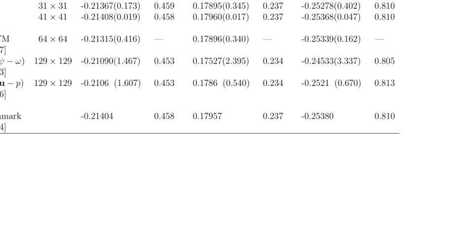
hori-zontal centrelines (Re= 100 and Re= 1000) are summarized in Tables 10–11. The

corresponding results obtained by the pseudospectral method [44], finite-difference

method [43,46] and finite-volume method [47] are included for comparison. The

IRBFN results are in better agreement with the spectral solutions than those

pre-dicted by the finite-difference and finite-volume methods.

Iso-vorticity lines of the flow for various Re numbers are shown in Figure 7. The

vorticity-contour values chosen here are the same as those in [43,44], i.e. _{-5, -4,-3,-2,-1,-0.5,0,0.5,1,2,3_}. The plots look reasonable when compared to those of [43] and [44].

not require any special treatment for the singularity at the two corners. In contrast,

when using the spectral collocation method, it is necessary to employ a subtraction

technique to remove the leading part of the singularity.

6

Conclusion

In the present chapter, an overview of high-order integral collocation techniques

using radial basis functions and Chebyshev polynomials is given. Three

impor-tant features of these techniques are: (i) Using Cartesian grids to discretize the

physical domain, (ii) Using point collocation to discretize the governing differential

equation, and (iii) Employing high-order integrated approximants to represent the

field variable, which result in effective numerical treatment schemes, particularly

for handling irregular boundaries, high-order differential equations and large-scale

domains. Several applications presented in this review illustrate the ability of the

integral collocation approach to solve complicated engineering problems.

Acknowledgement

This work is supported by the Australian Research Council.

References

1. Roache, P.J. Computational Fluid Dynamics. Hermosa Publishers:

Albu-querque, 1980.

2. Peyret, R.Spectral Methods for Incompressible Viscous Flow; Springer-Verlag:

New York, 2002.

3. Zienkiewicz, O.C.; Taylor, R.L. The Finite Element Method; McGraw-Hill:

4. Brebbia, C.A.; Dominguez, J. Boundary Elements An Introductory Course;

Computational Mechanics Publications: Southampton, 1992.

5. Mai-Duy, N.; Tran-Cong, T. Numerical solution of differential equations using

multiquadric radial basis function networks. Neural Networks. 2001, 14, 185–

199.

6. Mai-Duy, N.; Tran-Cong, T. Numerical solution of Navier-Stokes equations

using multiquadric radial basis function networks. International Journal for

Numerical Methods in Fluids. 2001, 37, 65–86.

7. Mai-Duy, N.; Tran-Cong, T. Mesh-free radial basis function network methods

with domain decomposition for approximation of functions and numerical

so-lution of Poisson’s equations. Engineering Analysis with Boundary Elements.

2002, 26, 133–156.

8. Mai-Duy, N.; Tran-Cong, T. Approximation of function and its derivatives

using radial basis function networks. Applied Mathematical Modelling. 2003,

27, 197–220.

9. Mai-Duy, N.; Tran-Cong, T. Indirect RBFN method with thin plate splines

for numerical solution of differential equations. Computer Modeling in

Engi-neering & Sciences. 2003, 4, 85–102.

10. Kansa, E.J.; Power, H.; Fasshauer, G.E.; Ling, L. A volumetric integral radial

basis function method for time-dependent partial differential equations: I.

Formulation. Engineering Analysis with Boundary Elements. 2004, 28, 1191–

1206.

11. Ling, L.; Trummer, M.R. Multiquadric collocation method with integral

for-mulation for boundary layer problems. Computers & Mathematics with

12. Mai-Duy, N. Indirect RBFN method with scattered points for numerical

so-lution of PDEs. Computer Modeling in Engineering & Sciences. 2004, 6,

209–226.

13. Mai-Cao, L.; Tran-Cong, T. A meshless IRBFN-based method for transient

problems. Computer Modeling in Engineering & Sciences. 2005, 7(2), 149–

171.

14. Mai-Duy, N. Solving high order ordinary differential equations with radial

basis function networks. International Journal for Numerical Methods in

En-gineering. 2005, 62, 824–852.

15. Mai-Duy, N.; Tanner, R.I. Solving high order partial differential equations with

radial basis function networks. International Journal for Numerical Methods

in Engineering. 2005, 63, 1636–1654.

16. Mai-Duy, N.; Tanner, R.I. Computing non-Newtonian fluid flow with radial

basis function networks. International Journal for Numerical Methods in

Flu-ids. 2005, 48, 1309–1336.

17. Mai-Duy, N.; Tran-Cong, T. An efficient indirect RBFN-based method for

nu-merical solution of PDEs. Numerical Methods for Partial Differential

Equa-tions. 2005, 21, 770–790.

18. Deng, J. Structural reliability analysis for implicit performance function using

radial basis function network. International Journal of Solids and Structures.

2006, 43(11–12), 3255–3291.

19. Ling, L.; Trummer, M.R. Adaptive multiquadric collocation for boundary layer

problems. Journal of Computational and Applied Mathematics. 2006, 188(2),

20. Mai-Duy, N. An effective spectral collocation method for the direct solution

of high-order ODEs. Communications in Numerical Methods in Engineering.

2006, 22(6), 627–642.

21. Mai-Duy, N.; Tran-Cong, T. Solving biharmonic problems with

scattered-point discretisation using indirect radial-basis-function networks. Engineering

Analysis with Boundary Elements. 2006, 30(2), 77–87.

22. Sarra, S.A. Integrated multiquadric radial basis function approximation

meth-ods. Computers & Mathematics with Applications. 2006, 51(8), 1283–1296.

23. Le, P.; Mai-Duy, N.; Tran-Cong, T,; Baker, G. A numerical study of strain

localization in elasto-thermo-viscoplastic materials using radial basis function

networks. Computers, Materials & Continua. 2007, 5(2), 129–150.

24. Li, C.; Wu, X. Numerical solution of differential equations using Sinc method

based on the interpolation of the highest derivatives. Applied Mathematical

Modelling. 2007, 31(1), 1–9.

25. Mai-Duy, N.; Khennane, A.; Tran-Cong, T. Computation of laminated

com-posite plates using integrated radial basis function networks. Computers,

Ma-terials & Continua. 2007, 5(1), 63–77.

26. Mai-Duy, N.; Mai-Cao, L.; Tran-Cong, T. Computation of transient viscous

flows using indirect radial basis function networks. Computer Modeling in

Engineering & Sciences. 2007, 18(1), 59–77.

27. Mai-Duy, N.; Tanner, R.I. A collocation method based on one-dimensional

RBF interpolation scheme for solving PDEs. International Journal of

Numer-ical Methods for Heat & Fluid Flow. 2007, 17(2), 165–186.

28. Mai-Duy, N.; Tanner, R.I. A spectral collocation method based on integrated

Computational and Applied Mathematics. 2007, 201(1), 30–47.

29. Shu, C.; Wu, Y.L. Integrated radial basis functions-based differential

quadra-ture method and its performance. International Journal for Numerical

Meth-ods in Fluids. 2007, 53(6), 969–984.

30. Mai-Duy, N.; Tran-Cong, T. An efficient domain-decomposition pseudo-spectral

method for solving elliptic differential equations. Communications in

Numer-ical Methods in Engineering, in press

31. Mai-Duy, N.; Tran-Cong, T. A Cartesian-grid collocation method based on

radial-basis-function networks for solving PDEs in irregular domains.

Numer-ical Methods for Partial Differential Equations, in press

32. Mai-Duy, N.; See, H.; Tran-Cong, T. An integral-collocation-based fictitious

domain technique for solving elliptic problems. Submitted.

33. Haykin, S. Neural Networks: A Comprehensive Foundation; Prentice-Hall:

New Jersey, 1999.

34. Micchelli, C.A. Interpolation of scattered data: distance matrices and

con-ditionally positive definite functions. Constructive Approximation. 1986, 2,

11–22.

35. Park, J.; Sandberg, I.W. Universal approximation using radial basis function

networks. Neural Computation. 1991, 3, 246–257.

36. Cover, T.M. Geometrical and statistical properties of systems of linear

in-equalities with applications in pattern recognition. IEEE Transactions on

Electronic Computers. 1965, EC-14, 326–334.

37. Madych, W.R.; Nelson, S.A. Multivariate interpolation and conditionally

pos-itive definite functions. Approximation Theory and its Applications. 1988, 4,

38. Madych, W.R.; Nelson, S.A. Multivariate interpolation and conditionally

pos-itive definite functions, II. Mathematics of Computation. 1990, 54(189),

211-230.

39. Smith, B.F.; Bjorstad, P.E; Gropp, W.D.Domain Decomposition Parallel

Mul-tilevel Methods for Elliptic Partial Differential Equations; Cambridge

Univer-sity Press: New York, 1996.

40. Gutierrez, R.H.; Laura, P.A.A. Vibrations of non-uniform rings studied by

means of the differential quadrature method. Journal of Sound and Vibration.

1995, 185(3), 507–513.

41. Wu, T.Y.; Liu, G.R. Application of generalized differential quadrature rule to

sixth-order differential equations. Communications in Numerical Methods in

Engineering. 2000, 16, 777–784.

42. Reddy, J.N. Mechanics of laminated composite plates and shells. Theory and

analysis; CRC Press: Florida, 2004.

43. Ghia, U.; Ghia, K.N.; Shin, C.T. High-Re solutions for incompressible flow

using the Navier-Stokes equations and a multigrid method. Journal of

Com-putational Physics. 1982, 48, 387–411.

44. Botella, O.; Peyret, R. Benchmark spectral results on the lid-driven cavity

flow. Computers & Fluids. 1998, 27(4), 421–433.

45. Poliashenko, M.; Aidun, C.K. A direct method for computation of simple

bifurcations. Journal of Computational Physics. 1995, 121(2), 246–260.

46. Bruneau, C.-H.; Jouron, C. An efficient scheme for solving steady

incompress-ible Navier-Stokes equations. Journal of Computational Physics. 1990, 89(2),

47. Deng, G.B.; Piquet, J.; Queutey, P.; Visonneau, M. Incompressible flow

calcu-lations with a consistent physical interpolation finite volume approach.

Table 1: Multiple boundary conditions: Condition numbers and errors by CSEs

nx×ny Differential Approach Integral approach

cond(_A) Ne(u) cond(A) Ne(u)

6_×6 4.4_×102 _1.23×10−1 _1.6×102 _4.84×10−3 8_×8 3.6_×103 _5.94×10−3 _1.5×103 _7.40×10−5 10_×10 2.0_×104 2.10_×10−4 _8.8

×103 4.20_×10−7 12_×12 9.2_×104 _4.46×10−6 _3.8×104 _2.40×10−9 14_×14 3.4_×105 _6.52×10−8 _1.3×105 _1.20×10−11 16_×16 1.1_×106 7.05_×10−10 _4.1

Table 2: Multiple boundary conditions: Condition numbers and errors by RBFNs

nx×ny Differential Approach Integral approach

cond(_A) Ne(u) cond(A) Ne(u)

7_×7 6.3_×105 _1.40×10−1 _2.4×102 _1.47×10−3 11_×11 3.4_×106 _1.22×10−1 _2.4×103 _1.61×10−4 17_×17 1.8_×107 1.46_×10−1 _1.8

×104 4.03_×10−5 21_×21 4.4_×107 _1.82×10−1 _4.5×104 _2.44×10−5 27_×27 1.2_×108 _2.33×10−1 _1.3×105 _1.41×10−5 31_×31 2.1_×108 2.64_×10−1 _2.3

×105 1.05_×10−5 37_×37 4.4_×108 _3.05×10−1 _4.9×105 _7.35×10−6 41_×41 6.7_×108 _3.30×10−1 _7.5×105 _5.95×10−6 47_×47 1.1_×109 3.63_×10−1 _1.3

Table 3: Non-rectangular boundaries: Condition numbers and errors by ICSEs

nx×ny cond(A) Ne(u)

Table 4: Non-rectangular boundaries: Condition numbers and errors by IRBFNs

nx×ny cond(A) Ne(u)