Automated RF Over Fiber Signal Measurement System

Theses Thesis/Dissertation Collections

12-2017

Automated RF Over Fiber Signal Measurement

System

Mageswaren Ravichandran

Follow this and additional works at:https://scholarworks.rit.edu/theses

This Thesis is brought to you for free and open access by the Thesis/Dissertation Collections at RIT Scholar Works. It has been accepted for inclusion in Theses by an authorized administrator of RIT Scholar Works. For more information, please contactritscholarworks@rit.edu.

Recommended Citation

AUTOMATED RF OVER FIBER

SIGNAL MEASURMENT SYSTEM

By

Mageswaren Ravichandran

A Thesis Submitted in partial Fulfilment of the Requirements for the Degree of Master of Science

in Telecommunication Engineering Technology Supervised by

Dr. Drew Maywar

Department of Electrical, Computer, and Telecommunications Engineering Technology College of Applied Science & Technology

Rochester Institute of Technology Rochester, New York

December 2017

Approved by

Drew N. Maywar, Associate Professor

Electrical, Computer, and Telecommunications Engineering Technology

Mark J. Indelicato, Associate Professor

Electrical, Computer, and Telecommunications Engineering Technology

Miguel Bazdresch, Assistant Professor

Dedication

I dedicate all my work family for all the support they have given me. I dedicate this work to all

Abstract

The demand for lossless data at a low cost has lead its way to use fiber optic in field of RADIO

FREQUENCY. This research proposes the automation technique which can be used in

RF-over-fiber measurements. All other automation technique used visual basic or Labview as the source,

this paper uses python an open-source language to create generic automation software. Python

optimized the code to run faster and gave advantage of modularity and portability. The code was

successfully developed and verified by the two-different test setup, which give an accuracy of

Acknowledgments

I thank Dr Drew Maywar for giving me the opportunity to study and work with him in this thesis

and various other research. I am personally grateful for this guidance, patience and support. I also

thank my fellow student and friend Mohamed Mafa and Son Pham for their guidance in this thesis.

I thank my parents for believing me that I can succeed in my goals and helping me in my tough

times. I greatly appreciate the Department Telecommunication Engineering technology for provide

me the opportunity to pursue gradation under the department. I thank all my fellow students and

friends who worked with me in the Centre for Photonic Communication lab for support me and

Table of Contents

Chapter 1-Radio Frequency over fiber ... 2

1.1 Introduction ... 3

1.2 Measurement of RF over Fiber ... 3

1.2.1 Compression Dynamics Range ... 4

1.2.2 Tone Tracking ... 6

1.2.3 Descriptive Statistics ... 7

1.3 Automating the measurement for RF over fiber ... 9

1.3.1 Why Python? ... 9

1.3.1 National instrument steps to automation ... 9

Chapter 2-National Instrument Automation Procedure ... 11

2.1 Introduction ... 12

2.2.2 Choosing the core Hardware ... 13

2.2.3 Determining the requirement Instrument ... 15

2.3 Selecting and arrangement of Hardware ... 15

2.3.1 Rack arrangement for the Hardware ... 16

2.3.2 Power distribution for the Hardware ... 18

2.4.1 Test Executive ... 19

2.4.1.2 Defining Variable/parameters ... 20

2.4.2 Code Module Development ... 21

2.4.2.1 Isolate code modules from the test executive operation ... 22

2.4.2.2 Encapsulate Commonly used functions ... 22

2.4.2.3 Creating Code Module Templates ... 22

2.4.2 Use source code control ... 23

2.4.3 Choosing the Instrument Driver Paradigm ... 23

2.4.3.1 Driver Options ... 23

2.4.3.2 PLUG AND PLAY driver ... 24

2.4.3.3 IVI instrument driver ... 25

2.5 Assembling the Test system... 26

2.6 Deploying the Test system ... 27

Chapter 3-Hardware Requirements for RF-Over-Fiber ... 28

3.1 Introduction ... 29

3.2 Schematic of RF over Fiber automation ... 29

3.2 LAB-BRICK Signal Generator ... 31

3.2.1 Features and application of Lab-brick ... 31

3.3 Keysight N5171B RF Signal Generator ... 32

3.3.1 Signal Generator Specification ... 33

3.4.1 oscilloscope Features ... 34

3.5 CXA N9000C Signal Analyzer ... 35

3.5.1 signal analyzer specification ... 36

3.6 The PC ... 37

3.7 Rack Arrangement ... 37

Chapter 4-Rf-Over-Fiber Measurement Software ... 39

4.1 Introduction ... 40

4.1 Global Variables and Name Schema ... 40

4.2 Initialization of hardware ... 41

4.2.1 LAB Brick ... 42

4.2.2 Example from the code ... 43

4.3 Flowchart and Code for Measurements ... 43

4.3.2 Test Executive Code ... 45

4.3.3 CDR Flowchart ... 46

4.3.3.1 instrument invoke code ... 47

4.3.3.2 Data acquisition code ... 48

4.3.3.3 CDR calculation code ... 49

4.3.4 Tone-tracking Flowchart ... 51

4.3.4.1 Marker loop code ... 52

4.3.5.1 Descriptive Statistics Code ... 56

4.4 Saving and Naming the Files ... 58

Chapter 5-Deployment of the Software ... 60

5.1 Introduction ... 61

5.2 Text executive results ... 61

5.3 CDR results ... 62

5.3.1 CDR outputs from Signal analyzer ... 65

5.4 Tone Tracking Results ... 67

5.4.1 Tone Tracking in Oscilloscope ... 68

5.5 Descriptive Statistics using Oscilloscope ... 71

5.6.3 File saving ... 73

Chapter 6-Conculsion ... 74

6.1 Conclusion ... 75

References ... 76

Table of Figures

Figure 1.1 CDR from textbook ...5

Figure 1.2 CDR from Research ...5

Figure 1.3 Tone Tracking ...6

Figure 1.4 a Oscillating value from scope ...7

Figure 1.4 b Oscillating value from scope ...8

Figure 1.4 c Oscillating value from scope ...8

Figure 2.1 Environmental Rack ...16

Figure 2.2 Portable Rack ...17

Figure 2.3 Rack Size ...18

Figure 2.4 Graph of driver ...24

Figure 3.1 Electrical Baseline ...29

Figure 3.2 Back to back Connection ...30

Figure 3.3 LABBRICK Function Generator ...31

Figure 3.4 Keysight Signal generator ...32

Figure 3.5 Keysight 12Ghz Oscilloscope ...34

Figure 3.6 Keysight Signal analyzer ...35

Figure 3.7 Research lab Rack Arrangement ...38

Figure 4.1 Test Executive Flowchart ...44

Figure 4.3 CDR Flowchart ...46

Figure 4.4 Instrument Invoke Code ...47

Figure 4.5 CDR main loop ...48

Figure 4.6 CDR Marker alignment and acquisition ...49

Figure 4.7 CDR automatic calculation ...50

Figure 4.8 Tone tracking flowchart ...51

Figure 4.9 Marker loop for acquiring tone ...52

Figure 4.10 Saving the data in to an array ...53

Figure 4.11 Tone tracking for signal analyzer ...53

Figure 4.12 Descriptive Statistic Flowchart ...55

Figure 4.13 Descriptive Statistic Code ...56

Figure 4.14 Marker assignment according to user ...57

Figure 4.15 Folder Creation ...58

Figure 4.16 File name time stamp creation ...59

Figure 5.1 Test executive run time window ...61

Figure 5.2 Oscilloscope CDR execution ...62

Figure 5.3 Loop start for CDR ...63

Figure 5.4 CDR plot before calculation ...64

Figure 5.5 CDR plot after calculation ...64

Figure 5.6 Signal analyzer CDR execution window ...65

Figure 5.7 b Back to back output for CDR using signal analyzer ...66

Figure 5.8 Showing the tone that are tracked ...67

Figure 5.9 showing the tone that are tracked in the signal analyzer ...68

Figure 5.10 Showing the values of the tone that are tracked ...69

Figure 5.11 Plot for tone tracking ...69

Figure 5.12 Plot for tone tracking from signal analyzer ...70

Figure 5.13 Descriptive statistics execution window ...71

Figure 5.14 Descriptive statistics output ...72

Table of Tables

Table 2.1 Variable Name ...21

Table 3.1 Keysight signal generator Features ...33

Table 3.2Keysight signal analyzer Features ...36

Table 3.3 Computer Configuration ...37

1.1 Introduction

The fiber optical is one major discovery in the human history. When people moved from

wired to wireless, they had the freedom hassle-free communication, but they had to pay a price.

The system became complex and costlier to build and deploy. As everyone know a message signal

needs a carrier to send and has the frequency of the carrier increases the noise in the transmission

decrease. The wireless system got up Ghz and it’s hard for generating such carrier. To overcome

all these problems and to increases the speed of the communication, Researchers have used light

has carrier to send message. The system was developed to send o’s and 1’s or commonly known

has digital communication. As ages pasted, there was many improvements in the system but still

used digital technology. The concept of RF (Sine –wave) over fiber was introduced and many

researchers have showed ways, How the fiber can be used in modifying RF signals. This is new

concept and there are only few measurement techniques to qualify the system.

1.2 Measurement of RF over Fiber

Every experiment requires a measurement technique to characterize the system. Likewise, RF over

fiber also has some measurement technique which can be used. This research is going to focus on

the technique like

1. Compression Dynamic Ratio

2. Tone tracking

1.2.1 Compression Dynamics Range

The compression dynamic is used to find harmonic distortion and intermodulation

distortion. This method is associated with gain compression and it used for single-tone input signal.

CDR is used for analysis of nonlinear system under excitation. The CDR follows power series

like Taylor Series

The Taylor Series for function 𝑓𝑓(𝑥𝑥) is

𝒇𝒇(𝒙𝒙) = �(𝒙𝒙 − 𝒂𝒂_𝒏𝒏! )

𝒏𝒏 _{𝒅𝒅𝒏𝒏𝒇𝒇}

𝒅𝒅𝒙𝒙𝒎𝒎 ∞

𝒏𝒏=𝟎𝟎

The application of the Taylor series has limitation like it can only be used has analysis a small

excitation and the system should nonlinear without memory. The meaning is that the output power

of the signal should be a function of input signal.

The linearity of the circuit can be analyzed using Taylor series when the output depends on the

input as follows

Vout(Vin) = a0 + a1(Vin - Vb) + a2(Vin - Vb)2 + a3(Vin - Vb)3 + · · · ,

According to the author Jason D. McKinney, “The x-dB CDR is defined as the range of input

powers over which the signal is above the noise floor at the output, and the output power is

compressed by x-dB or less relative to a linear response”[4]. Mathematical representation of the

compression dynamic range is

Where 𝑃𝑃_{𝑥𝑥𝑥𝑥𝑥𝑥} is the output power at x-dB-compression. The commonly known as linear dynamic range.

𝑪𝑪𝑪𝑪𝑪𝑪𝒙𝒙𝒅𝒅𝒙𝒙 =𝑷𝑷𝒙𝒙𝒅𝒅𝒙𝒙𝟏𝟏𝟎𝟎 𝒙𝒙 𝟏𝟏𝟎𝟎⁄

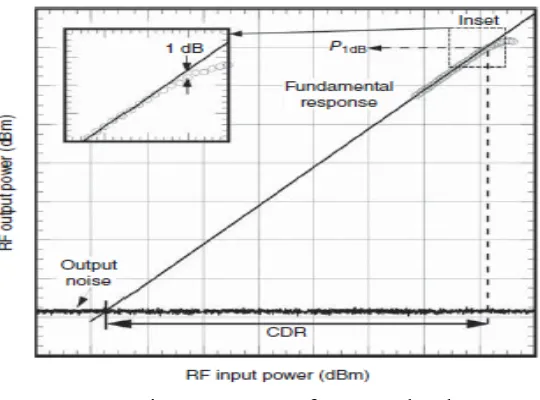
Measuring the CDR at 1dB shows the fundamental response of the system under test and the output

noise. The fundamental response can be measured using the signal source and a spectrum analyzer.

The output noise can be measured using the spectrum analyzer without the source. Figure 1.1

shows the graphical representation from the fiber optic experiment conducted by the author and

Figure 1.2 is graphic of CDR at 1dB obtain by our research.

Figure 1.1 CDR from text book

Source: Fundamental of microwave photonic

1.2.2 Tone Tracking

Tone tracking is simple concept which is used in the measurement of Radio frequency. We

all know that the transmitted signal is going to receive with some noise and distortion. The tone

tracking is the method we used to track all the harmonic distortion.

This is important because the signal is altered both in time and frequency domain. The

addition of new frequency alters the signal completely, this will affect the outcome when the signal

is sampled for further processing. The tone tracking is also a function of input power. As the input

power increases the output power of each harmonic-tone also increase. It also helps us to find what

type of frequency is added to the signal and how it is going to change in time domain.

The tone can be measurement using an input source and signal analyzer. We can also use

oscilloscope with Fourier transform feature. Figure 1.3 is output image from the signal analyzer

with six tones. The Tone 1 is the fundamental tone for the output and rest output other different

tones.

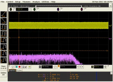
1.2.3 Descriptive Statistics

Descriptive statistics is concept which is introduced by our research. This method was

developed due an issue faced by the experiment. When an input power was set, the output power

in the instrument was oscillating. To get an average output power of the signal, we came out with

concept of descriptive statistics. This is a simple math averaging technique, where the output

power is measured in equal interval of time keeping the same input power. This measurement is

used to find the average output power for the signal which can be used for various other offline

processing.

The descriptive statistic(DS) can be measured for any tone. The measurement can be

obtained using oscilloscope or signal analyzer. Figure 1.4a, b and c are showing the output power

oscillation of the same input power.

Figure 1.4 b Oscillating value from the scope

1.3 Automating the measurement for RF over fiber

The focus of this thesis is to automate above mentioned process. There are many ways in

automating, this research is going to focus on the National Instrument steps to automation. The

research is going use python an open source language with some libraries and NI automation guide.

1.3.1 Why Python?

Python is the widely used scripting language when compared to others. It has many

libraries which are open source. Python is interpreter language which make the scripting simple.

The syntax is easy, and all the instrument drivers support python.

1.3.1 National instrument steps to automation

National Instrument are the leading software company in the field of automation. They

developed many instruments and software for automation. The have well published article on how

automation can be implemented. The 5-step automation are

1. Identifying the scope of the test system

2. Selecting and arrangement of Hardware

3. Designing Software

4. Assembling the Test system

5. Deploying the Test system

These are common procedure followed all the test Engineering. This study will further explain

about the implementation of the NI test standard using the open sourced python language. All the

code for more update and new feature additions. The python language helps the portability and

2.1 Introduction

As previous mentioned the NI are the leading developer of automation software and

hardware, we are following the guide to develop an automation software for lab and industry

purpose. This chapter will give detailed explanation of various steps involved in automation.

2.2 Identifying the scope of the test system

Once all the test has identified and performed manually. We know all the constraints as well

as priorities. Now we are ready to perform automation. The first step is to determine the

measurement requirement for the device under test. This section will explain the various factor to

consider in the measurement need of the test system.

2.2.1 Identifying the scope of the test system

The initial step in identifying the scope of any system is to identify the scope of the system. That

is, whether the system is going to test a sole product or entire group of products.

For example, when a sole product is tested for specific parameter. It is simple as the measurement

will be setup for testing with high-speed measurement units. The result from this setup will be

accurate and will have high resolution. But when more than one device is going to be tested, then

the system should have a range of specification to adopt all the device under test (DUT) parameters.

Determining this will help the engineers to determine the type hardware and software. They should

consider the type communication medium between the instrument and software. There is also

various other consideration that needs to be taken care like

• Budget and timeline

2.2.2 Choosing the core Hardware

Once all the measurement need for the system is determined, then hardware framework

architecting is started. Many researchers start matching their measurement needs to

instrument available on the market. The better approach suggested by NI is pinpoint a

suitable test platform that can serve as the core or nucleus of the test system. They have

suggested factor to consider when choosing the core platform

• Processing power and data throughput

o Considering the computational power required for the controller

• Scalability

o Scalability is one of the crucial factor to consider as it helps in any further modification to the system.

• Measurements Diversity

o If the platform serves as a multi-core test system, then it should be addressed. In general, the test system should accommodate 80% of all the test system

measurement needs

• Communication with other Buses and Instruments

o All the instrumental bus and platform as it owns distinct advantages and disadvantages. National instruments suggest building a hybrid system based

on multiple instrument bus, so that we can take advantage of the strength of

different measurement system. This give flexibility to build a complex and

• Timing and synchronization

o All instrument should be synchronized by send trigger and sharing clock, otherwise there can mishandling of data.

• Lifetime

o If the engineers are planning for long term test system, then they should use the system which are not in the end of life or end of sales. These systems need

constant calibration to perform at their highest efficiency. Using EOS system

will affect the process and it will be hard to find replacements.

There is detailed example provided by the NI. I am attaching it below:

These six criteria helped NI engineers select a core platform for the automated test system they

used to assess the CompactRIO I/O modules. The following is an evaluation of test system needs

based on the criteria:

1. Processing Power and Data Throughput: This system required a multicore processor and a

high-speed data bus that could support the expected data analysis.

2. Scalability: Because the CompactRIO product line is continually evolving and growing, it was

essential for the system to use a core test platform that is highly scalable to be able to add new

functionality for future CompactRIO platform releases.

3. Measurements Diversity: The CompactRIO tester had to be capable of testing the large variety

of I/O types on the more than 50 modules for the CompactRIO platform. These include ±80 mV

thermocouple inputs, ±10 V simultaneous-sampling analog I/O, 24 V industrial digital I/O with up

to 1 A current drive, differential/TTL digital inputs with 5 V regulated supply output for encoders,

modules need to address, the NI engineers also required the tester to make a wide range of

measurements.

4. Communication with Other Buses and Instruments: The CompactRIO platform is continually

growing and future product plans are hard to predict, so NI engineers needed a tester with a high

level of flexibility to accommodate a vast range of instruments that are based on different buses.

5. Timing and Synchronization: Because there is a possibility for multiple instruments based on

different buses to coexist in the system, the core platform needed to seamlessly synchronize these

instruments.

6. Lifetime: The test system was designed to work for the entire lifetime of the CompactRIO

product line, and thus required a core platform that is continually growing and whose components

were likely to be serviceable and replaceable for several years.

2.2.3 Determining the requirement Instrument

As the scope of the measurement and core hardware platform is determined. The next step

is to find the proper instrument. it is always better to select instrument based on the measurement

or stimulus rather than instrument type.

2.3 Selecting and arrangement of Hardware

In this section, we will be looking for the selection of rack to arrange all the instrument.

this is important because as the frequency increases the loss also increases, so arranging the

2.3.1 Rack arrangement for the Hardware

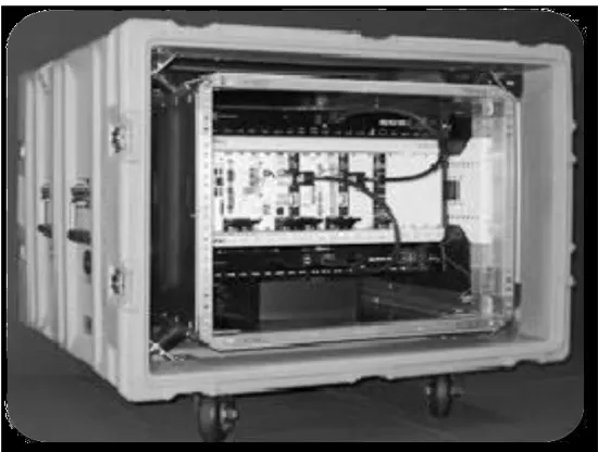
Rack is enclosure that are typically used to store instrument, fixture and cables. Others can

provide the necessary cooling and ventilation to prevent from overheating of the measurement

system. The rack can be chosen according to the environmental usage, portability, size and cooling

1.

Environmental use

The type of rack to be chosen should be depending the environment in which the

system is used. For example, if the system is kept in the rugged environment like in a

helicopter or other military vehicle then the rack should withstand the heat and pressure to

safeguard the equipment. Figure 2.1 is an example from NI of rugged testing rack.

2.

Portability

The factor to be consider is portability of the rack. There test which is conducted in

stationary but there are measurement system or equipment which is in constant move.

Example, The radio use in military for communication. Figure 2.2 is portable rack image

from NI

3.

Size

Rack size is important if the system is going to expand. The rack should be based

on the Electronic Industries alliance(EIA) standard as the test instruments are build

according to those standards. Figure 2.3 is image from NI explaining the size of the racks.

4.

Ventilation

The system in measurement unit generate lot of heat. It is better to consider the

cooling factor. The cooling method is going to depend on the environment. There are two

type of cooling rack

Option 1: - If the environment is dust free and air tight then the perforated rack can

be used which ventilation that can provide channel for hot air to escape

Option 2: - If the environment is outdoors then fully sealed rack with proper cooling

fan and hot air channel to reduce the temperature inside the rack

2.3.2 Power distribution for the Hardware

The instrument power is connected to the terminal strip in the rack and the terminal strip

is the connected to the main power socket in the wall or on the ground under the rack. The PDU

should be able to withstand the load from the rack. The PDU should be consider with expansion

and should be occupied 70% of its total watts capacity. Other safely precaution like emergency

power off and circuit breaker should be considered while deploying the unit.

2.4 Designing Software

The software in the test design and building is a crucial part because the top three layers in

the developing test system is software. This section in the test layer explains the importance of the

system management involved in the development. The following explains the role of test executive

and how it interacts with other two software.

• Test Executive: - This run a series of test quickly and consistently in a predefined

progression. This mode run the common operation for all devices, such as serial

number entry, initialization and save the outputs. By allowing this increases the

time for the developer to design his test code.

• Code Module: - This module implements the measurement I/O, high-speed looping

and analysis. This help in build a code module with high modularity and reusable

code. It also helps the application development environment to develop the code

module

•

the software routine to run on the programmable instruments. Each instruction set

contain the configuration, reading from, writing to and triggering the instrument.

This driver reduces the time from programmer by eliminating the need to learn the

programming protocol

2.4.1 Test Executive

There test executives from third part which will help the programmer to deploy the code

on them to run. There are also test executive which are build in-house for accuracy and speed. The

capacity and efficiency. This part of test executive is guide to those who want to develop in-house

software for their automation by NI.

2.4.1.1 Sequence Reuse/Section

Whenever there is a new function is introduced try reusing the same specification or

functionality. Conditional statement can be used to limit the usage of the test run or to make any

new changes while the test runs. If more changes occur in the test, use the second test sequence to

implement clarity tot the system.

The NI guide have given detail implementation of test executive for the GUI of the test

system which is not concentrated in this research.

2.4.1.2 Defining Variable/parameters

According NI, variables are data storage construct that can be used to store and share

information. Variables can be implement globally or locally to a specific sequence. The creation

of variable should have defined by the test executive and it should be tracked for the values and

properties. The implementation of variables is particular to the language used and the engineers

should be informed of all the variables used in the test. The variables can be defined as

• Local Variables: - They store data for specific sequence and it not shared out the

sequence or function. This type of variable is used pass values that required to

perform with the function

• Sequence file global variables: - The sequence file global variable is used store data

for the entire sequence of the test set and any other sequence can access the value

• Station global variables: - This global variable is specific to automation process as

it will contain the data of the configuration of the instruments, initialization of

instruments and other data required for the entire test process to complete. These

variables are passed between the modules, sequence and functions.

Standard variable naming convention

When developing the name for variable consider the new member in the further and

implement the naming convention for the variable. The NI have suggested the table of example on

how the name convention can be.

2.4.2 Code Module Development

Code module is the section where the main code developed by the programmer get

executed. This also called as development modules. The flexibility here defines the modularity of

the software. NI have suggested a best guideline on how to develop a code module.

2.4.2.1 Isolate code modules from the test executive

operation

As the name explain the code module should be isolated from the test executives.

Developing modular for each measurement and reusing the same code for analysis leads to fast

accusation. The separation of test executive and code module help using the same code with the

different test executive. This research has developed its own test executive and code module which

will be explained in the later chapters.

2.4.2.2 Encapsulate Commonly used functions

The encapsulation here means separating the common post-test function from the actual

function. For Example, consider a function that bring waveform data and measures the

characteristic of it. Then the post function routine should be considered to measure all the

requirements on the acquired waveform. Then two separate function should be created for accruing

and other for testing. To use other code modules which are related to the waveform should be

encapsulated for future use.

2.4.2.3 Creating Code Module Templates

This is modules is for the closed code situation. With the template programmers can build

specific part and send to other programmer, so he can create his work. Another use is that if the

programmers want to have common flow of code in all the work then a template can be use. The

best example is NI Labview where common template is used to create the skeleton of the program

2.4.2 Use source code control

This method used many industries to develop large test system. Its help the managers to

control and track the changes in the code. some common use of source code controls mention by

NI are: -

• Tracking and identifying changes to code

• Distributing code modules to development teams

• Detecting and resolving conflicting changes to source code

• Providing centralized access to all versions of code

• Integrating changes to the master code depot

2.4.3 Choosing the Instrument Driver Paradigm

Choosing or developing an instrument driver strategy is not difficult job but it is necessary

for one to understand how they work. The research has faced bottleneck due to selection of

improper drivers which will be explained in the upcoming chapters. If the setup uses more than

one vendor, then developers might have to use all the driver without conflicting. The NI have

developed a common driver known as” VISA” which can be used for all the instrument from

different vendor. This section helps in the approaches on the instrumental drivers.

2.4.3.1 Driver Options

According to NI guide “Instrumental driver is a set of software routines that control a

before they instruction set that helps the developer to increase their development time by

eliminating the need to learn programming protocol for each instrument. There are three types of

driver available.

1. Direct I/O

2. Plug and Play

3. IVI

Figure 2.4 gives the graphical advantage of the drive and how to approach the driver and

help programmer to decide which driver would be suitable for there automation.

2.4.3.2 PLUG AND PLAY driver

Plug and play driver are driver which are automatically detected by the computer. The

simplest example is a pen drive, when it connected to computer it is automatically detected and

we start using it.

The advantage of this, the developer need not waste his time in search of the driver for the

instruments. They are already programmed in the operating system. The major disadvantage of

this the driver will not be update for long time and there are only few instrument support plug and

play.

2.4.3.3 IVI instrument driver

In development environment update drivers constantly is time consuming job and error can

occur in the process. The constant re-development, re-verification and re-documentation is always

there in a development environment. For such situation, we use Interchangeable Virtual

Instruments(IVI). This driver is maintained by IVI foundation, there key feature is they support

multiple vendors.

Other advantages are architectural longevity and usability.

2.4.3.4 Direct I/O Driver

Direct I/O is simple low-level method for the programming instruments. It follows IEEE

488.2 standard that defines the standard programming command set and syntax for Direct I/O.

This is only used when the plug and play or IVI instrument are not available. It can also be used

for the following: -

• Updating an old system

• Send few command to instrument

• Not developing the command and using the SCPI instruction

The latest development the Direct I/O communication is Virtual Instrument Software architecture

(VISA) API. It is industry standard instrumental communication protocol developed and

The Visa can support ASCII string for communication and it can use USB, GPIB and

ethernet. It provides interface independence and switching between devices are fast and help user

to control many devices in a single language.

This Research uses VISA for the instrumental communication and example on how it is done will

be shown the upcoming chapters.

2.5 Assembling the Test system

This is the crucial part of all in the automation process. Once all the device and driver are

finalized, then we must assemble the entire system. This section will give detail information of

four-step assembling of the test system.

1. Assembling the Components: - The component should be placed close to each other to

decrease the cable loss. They should be place according to rack unit mentioned in their

guide to increase the cooling effect of the process. This help to reduce the thermal noise in

the system.

2. Building and Routing Cables: - There some cables which will not withstand the power

requirement of the instruments, so It is always safe to use the cable given by the

manufacturer to power up the devices. The connecting or communication cable are

different, and they have a loss profile according to the frequency needs. It is better to know

the profile and make connection to get minimum loss in the results. When coming to

grounding, proper grounding help in unwanted damages to humans and the instruments. It

will also increase the resolution of the results.

3. Installing and Activating the Software: - This section is important when the software is

installed. The software installation document will provide the necessary information for

the user. It is always good to about the license strategy about the software for further

requirement. Whether it is lifetime or annual renewal software, so that the plan cane be

made according.

4. Validating the Test: - It necessary to test all the driver and other software modules to help

with test set to validate them. There are several documented techniques by NI to validate

the test setup.

Once all these are done, it is time to deploy the system.

2.6 Deploying the Test system

Once all the systems are analyzed and fabricated, it’s time to deploy the system.

Deployment presents several questions as the system was developed in a closed environment.

There will be few failures initially but after handling those error system is good to go. There few

factors to be considered while deploying. They are

1. File Extension

2. File location and naming

3. Source control Method

4. Safety

5. Power

3.1 Introduction

The automation process is separated into two chapter. This chapter to going to explain the

hardware contribution for the thesis. The next chapter is going to explain about the software

contribution. The chapter 3 contain the schematic diagram of experiment used to test the

automation software and hardware used. The chapter also contains the Rack-arrangement of

devices to yield minimum loss. All the information provided in this chapter are acquired from the

manufacturers website.

3.2 Schematic of RF over Fiber automation

The Figure 3.1 is simple Electrical baseline connection where the function generator is

directly connected to the oscilloscope and then later it is connected to the spectrum analyzer. Both

Signal generator and accusation unit is connected to the computer using a ethernet cable. The

accusation unit is an output device which is used to view the plot or collect data like oscilloscope

or signal nanylzer. The PC and the instruments are communication using the VISA driver. This is

used a test setup for the code

Signal Generator

Oscilloscope

Computer Electrical Cable

Ethernet Cable

The Figure 3.2 is the actual RF over fiber setup experimental setup. The continuous wave

from the tunable laser given as input to external modulator (MZM) which is also getting to input

signal for the signal generator. The modulated output of the MZM-modulator is connected to the

input of the Photodiode. The photodiode is the device which converts the optical signal back to

electrical RF signal. This output from PD is connected to the oscilloscope or signal analyzer to

view the output. Both the Signal generator and oscilloscope or signal analyzer is connected to PC

for automation. The automation code is written in python.

Oscilloscope Signal Generator LASER Electrical

Photodiode

External

Modulator

Ethernet Optical

3.2 LAB-BRICK Signal Generator

The LAB-brick LSG-222 is a USB programmable hand held low-cost signal generator. It

has a frequency range of 500MHz to 2200MHz an phase noise off of -110Hz. The unit offers a

100kHz frequency step size. It also offers configurable frequency step and 0.5dB power control.

The LSG is powered using the USB cable and the software which only runs in windows. A GUI

based controller is provide with the unit and they also offer SDK for any future development. The

device doesn’t support python and we had develop our own controller with the .dll files.

3.2.1 Features and application of Lab-brick

These are the features and applications are listed in the LAB brick website

• USB powered and controlled

• Includes easy-to-install-and-use GUI

• Programmable frequency stepping

• Operate multiple devices directly from a PC or self-powered USB hub

• Autonomous operation from USB hub or battery pack

• Easily programmable for ATE applications

• Robust aluminum construction

• Customization available for unique requirements

• API DLL, Linux and LabVIEW compatible drivers

3.3 Keysight N5171B RF Signal Generator

The Keysight N5171B has a frequency range of 9kHz to 3GHz.They can achieve faster

throughput and greater uptime. The output power from the generator is verified as

industries-leading technology. Pure sinewave is produced by the system. They can switch between frequency

in less than 800uS. They can produce modulation scheme like AM, FM and PM. These

modulations are software generated.

3.3.1 Signal Generator Specification

The table 3.1 contain the specification of the signal generator

Frequency 9 kHz to 6 GHz

Output Power @1 GHz -144 dBm to +26 dBm

Phase Noise @1 GHz (20 kHz offset) -122 dBc/Hz

Frequency Switching ≤ 800 µs

Harmonics @1 GHz <-35 dBc

IQ Modulation BW Internal/External n/a

Non-Harmonics @1 GHz -72 dBc

Sweep Mode

List

Step

Baseband Generator Mode n/a

Software-General Purpose

AM, FM, PM

Pulse

Pulse Train Generator

Software-Detection/Positioning/Tracking/Navigation n/a

Frequency Modulation-Maximum Deviation @1 GHz 10 MHz

Frequency Modulation-Rate @100 kHz Deviation DC to 7 MHz

Phase Modulation-Maximum Deviation in Normal

Mode

1.25 rad to 20 rad

3.4 Keysight Infiniium DSO81704B Oscilloscope

The oscilloscope has a bandwidth of 12GHz with 4 analog channels input. It has sampling

rate up to 40Ga/s. The display of the scope is a XGA display with 256 levels of intensity grading.it

has noise floor of 387uV @ 5mV/div and trigger jitter less than the 500fs(rms). The scope can go

display the points up to 6 decimal value. The oscilloscope has capability of achieving accurate and

repeatable values. The limitation of the system is, it can only show 2 markers

3.4.1 oscilloscope Features

• 12 GHz bandwidth real-time oscilloscope with up to 40 GSa/s sample rate

• Up to 2 Mpts MegaZoom deep memory at 40 GSa/s sample rates

• System bandwidth of 12 GHz with InfiniiMax II 1169A probing system

3.5 CXA N9000C Signal Analyzer

The Signal analyzer has bandwidth of 3kHz to 13.6GHz. It has the capability to accrue

value up to 8 decimal points. It has harmonic tables and it can even calculates phase noise for the

components. The device has ability to display 12 markers. It has multiwindow capabilities and it

can be controlled by web interface.

3.5.1 signal analyzer specification

Frequency 13 Ghz

Maximum Analysis Bandwidth 25 MHz

Bandwidth Options 10 standard, 25 MHz

Maximum Real-Time Bandwidth n/a

Real-Time Bandwidth Options n/a

DANL @1 GHz -163 dBm

Phase Noise @1 GHz (10 kHz offset) -110 dBc/Hz

Phase Noise @1 GHz (30 kHz offset) n/a

Phase Noise @1 GHz (1 MHz offset) -130 dBc/Hz

Overall Amplitude Accuracy ±0.5 dB

TOI @1 GHz (3rd Order Intercept) +17 dBm

Maximum Dynamic Range 3rd Order @1 GHz 111 dB

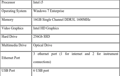
3.6 The PC

We are using the Intel i5 PC for automation. The PC is installed with VISA drivers and

Pychram Community Edition IDE. The Pychram is software in which the python scripts are coded.

The scrip for automation are written in Python Language. The table below is spec for the PC

Processor Intel i5

Operating System Windows 7 Enterprise

Memory 16GB Single Channel DDR3L 1600MHz

Video Graphics Intel HD Graphics

Hard Drive 256Gb SSD

Multimedia Drive Optical Drive

Ethernet Port

3 ethernet port (1 for internet and 2 for instrument

connections)

USB Port 6 USB port

3.7 Rack Arrangement

There 2 full size racks and 1 half size rack in the Lab. The left full-size rack contains instruments,

such as signal generator and pattern generator. The right full-size rack contains instrument like

oscilloscope and Signal analyzer. The bottom of Rack 2 has photodiodes and power supply. The

half size has the laser for the external modulator. These instruments are place in these orders to

reduce the cable loss.

Figure 3.7 Research Lab Rack Arrangement

Pattern generator

Signal analyzer

Signal generator

Microwave generator

Power Supply _{13Ghz Signal Analyzer} 1Ghz Oscilloscope 12Ghz Oscilloscope

Photodiode

Power supply

Rack1

Rack 2

4.1 Introduction

This Chapter is going to give a detail insight of the software developed to automate the

measurement process. All the devices are connected using ethernet to the hub or network switch

and the pc is also connect to the hub. Each device is given a static internet protocol (IP) address,

so they can be accessed. The code is separated into two sections known as test executive(TE)and

code module(CM). As the chapter 2 explains TE is base to execute the code module.

4.1 Global Variables and Name Schema

In this research, the global variables are allocated to the instrument drivers. These drivers

help to initialize the instrument for communication. The local variables are used to pass the value

between the code modules. For example

Global variables: - instscope, instgen, instanalyser

Local variables: - pow, markercdr, markertone , harmo

The name is also important because it going to help future students to expand the code.

The name schema was chosen in the way that when a variable is defined, the name will provide

NAME VARIABLES

Input power level pow

Output power level powout

Harmonics or tone value harmo

Scope driver value instscope

Signal generator driver instgen

CDR marker values markercdr

Excel sheet name Workbookname

4.2 Initialization of hardware

The hardware initialization is the important part in the automation process. Choosing a

wrong driver would wreck the entire process. This thesis uses VISA driver and Pyvisa library for

the connection. The Lab-brick generator does not support VISA drivers, so we used .dll driver

given by the manufacture and ctype library in python to invoke the device.

Initially we use USB connection for all the instrument, but they gave timeout error. So, we

started using ethernet connection which gave advantage of assign a specific IP address to all

devices. To write a command to instrument we use “write” and to send and receive command we

use “query” The general example for the VISA connection is

import visa

rm = visa.ResourceManager()

rm.list_resources()

inst = rm.open_resource('GPIB0::12::INSTR')

print(inst.query("*IDN?"))

4.2.1 LAB Brick

The lab brick will be using the below mention invoke command set to communicate and it

will use the device name with prefix of “fn” to send command t the device. We are using LSG

222-20 signal generator

Invoke example:

from ctypes import c_int, c_double, byref, c_char_p, CDLL

CDLL_file = "VNX_atten.dll"

va = CDLL(CDLL_file)

va.fnLSG_SetTestMode(False)

##Get Device Info

print va.fnLSG_GetDevInfo(c_char_p(1))

Command example:

fnLSG_GetMaxPwr(Devices[0]), - to get power value

4.2.2 Example from the code

Signal Analyzer:

rm = visa.ResourceManager()

list1 = rm.list_resources()

instanalyser=

rm.open_resource('TCPIP0::192.168.255.15::inst0::INSTR')

Signal Generator:

rm = visa.ResourceManager()

list1 = rm.list_resources()

instsiggen=

rm.open_resource('TCPIP0::192.168.255.25::inst0::INSTR')

Oscilloscope:

rm = visa.ResourceManager()

list1 = rm.list_resources()

instscope = rm.open_resource('TCPIP0::192.168.255.5::inst0::INSTR')

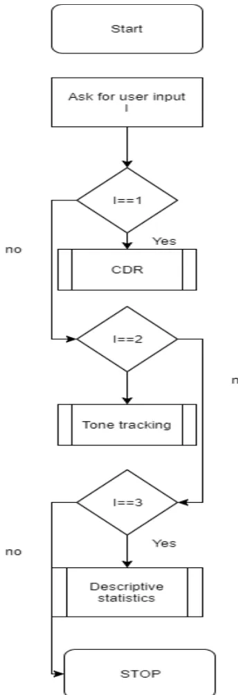
4.3 Flowchart and Code for Measurements

The flow chart is pictorial representation of the algorithm used to automate the process.

This section will show the flow charts and code of all three measurements used. The software code

4.3.2 Test Executive Flowchart

Test executive is main program or function which is executed first, this TE calls other

function known as code modules to complete the code. Figure4.1 is as simple flowchart explaining

TE and I will change in future, if any add feature is added

4.3.2 Test Executive Code

Figure 4.2 is a self-explanatory image which contains all other program within. The TE

assigns the global variable and pass it to others. This is a simple logic test executive.

4.3.3 CDR Flowchart

The flowchart of CDR contains 3part. The first part is the CDR_calculation which invoke

the measurement instruments. The second part is harmonicXcdrmaker, it calculates the marker

position and value. The final part is CDR range calculation which find the CDR of the system.

4.3.3.1 instrument invoke code

The CDR invoke code helps to set the parameter to the instrument. The input device is the

keysight signal generator and the output measurement device is infiniium scope or keysight signal

analyzer. As per the flowchart the loop of the code goes till the values in the range of input power

levels. Below is the snippet of the code.

In the Figure 4.4, The marker function and the signal analyzer are invoked using the input

command. This entire code is modules, we are passing the scope and the signal generator global

variable to module to send command to the device. In theabove code we are asking for the input

of the power range and step size. The “powrag” variable is used generate the range of values.

Variable “Freq” is set to float and the get the frequency value from the user.

4.3.3.2 Data acquisition code

In the Figure 4.5, This the loop part in the flow chart. The code checks for the power range is

within the selected safety limit. If it is in the safety limit, then It send the command ”2Ghz POW

10DBM” to the signal generate. Once the value is set, the code calls for the function

“harmonicXcdrmark”.

The figure 4.6 above is the second part in the flow chart. This part of the code is used set x axis

for the marker position and get the y axis of the marker. All these are return to main mode and

saved in array.

4.3.3.3 CDR calculation code

This section of the code is crucial as it going to calculate the CDR for the acquired data. The CDR

will automatically calculates or asks from the user to input the starting power range. This condition

is set such that, some abnormal value can be neglected in the calculation of CDR. Figure 4.7 is the

code for the automatic calculation of CDR. The code also takes care of the cable loss by asking

the user to mention the cables loss value. The default section is zero for cable loss. The user also

can set any compression value for the CDR calculation. The default value for compression is 1dB.

4.3.4 Tone-tracking Flowchart

The tone- tracking flowchart has two parts. The first part is going to be same has CDR,

which is dealing with the instrument initialization. This known as code reusability, which helps

the system to process faster. The second part has loops for the marker which I going to move along

the x axis to get the data. The loop is used because the scope has only to markers, which limits the

process to get only six harmonic values.

4.3.4.1 Marker loop code

The instrument initialization is going to use the same code from CDR. The marker loop is

a module which is used to track all the user specified tone. The coed for tracking of user specified

tone is going to different for the scope and signal analyzer, because the scope has only to two

markers and signal analyzer has 12 markers. Due to this constraint in scope we needed to limit the

tone tracking to the six tones per input power.

Figure4.9 is for the oscilloscope. The module parameter “orderhar”, it gets the input from

the user for the tone values. Using that variable, the For-loop cycles to get all the values and save

it in a signal array.

The values then separated and saved in others different arrays as individual tone for each

power levels. All the saved values are plotted with different markers.

Figure 4.10 Saving the data to an array

The image above is the tone tracking code for the signal analyzer. The first loop in the code places

all the marker in the user defined position. The loop is normal loop which changes the input power

4.3.5 Descriptive Statistics Flowchart

The descriptive statistics doesn’t have multiple parts, it is single modules which use same

algorithm for both the oscilloscope and signal analyzer. This method is mainly used for the

Oscilloscope has it output was the one which kept on varying. The figure below is the flowchart

of the descriptive statistics

4.3.5.1 Descriptive Statistics Code

The code for descriptive analysis is different from other two, as it doesn’t dependent on the

loop of input power. The code doesn’t have any other module except a main module which

contains all the necessary information. Figure 4.13 Is going set the input power and frequency to

the signal generator.

Since the scope had only two markers we set the markers at user specified harmonic tone and it

will also ask the user for number of values to recorded. The loop in the code goes for user specified

number of time and records all the value in an array. Then this array is passed to the test executive

and the output is recorded in an excel sheet for future processing.

4.4 Saving and Naming the Files

This section will help to understand how the files are save and named. The code tries to

create a folder name “DATA”. Within these folders another folder name “date” is created. This

date change day to day as it follows the date. The files are given the name according to

measurement and time at which the measurement is started.

Figure 4.15 is part of code which is used to create the folder. This system scan for these

folders every day to avoid duplications.

Figure 4.16 is the part code which get the time stamp and name of the measurement for the excel

sheet.

5.1 Introduction

This chapter will show all the results generated using the code. The first half results are

from the electrical baseline and the second half is going to show the experimental results. This

chapter also shows on how to use code.

5.2 Text executive results

The test executive is first program which runs when a code is executed it. Figure 5.1 is the

windows seen by user. It will list all the test measurements which are available.

5.3 CDR results

When the CDR is chosen in the figure 5.1. The instrument variables are passed, and the

interpreter asks for the user inputs. The Figure 5.2 is the output the user sees. It will ask for the

starting range of the power level and It will ask for the step size and final power value. Once all

the data are entered. It will ask for the input frequency value. The first line of the output will show

the devices chosen and it will display the serial numbers of it.

In Figure 5.3, the loop process starts, as it display the “ FREQ 2.0GHz;POW -10dBm”. Before the

loop is user input for the for selecting which frequency tone to follow

Once the Figure 5.4 is shown, the program asks the user for manual selection or

automatic selection of areas for the CDR. If the user, choose automatic then the

following result will be shown.

Figure 5.4 CDR plot before calculation

Figure 5.4 and Figure 5.5 are the results of electrical baseline circuit. This graph is

used as a calibration to the code. The code also asks for the user if any cable loss is

present in the circuit.

5.3.1 CDR outputs from Signal analyzer

Figure 5.6 is the execution window of the CDR calculation for the Signal analyzer. As it shows

the device used in the program. The rest is all same as oscilloscope

Figure 5.7 a Electrical baseline output for CDR using Signal analyzer

5.4 Tone Tracking Results

In the test executive, when the “tt” option is selected the following output windows is show.

As mention in the previous chapter, the tone tracking module uses the same code of the CDR with

slight modification. Figure 5.8 is the output windows of the tone tracking.

Figure 5.8, show the tone which are tracked in the code. This can be automatically assigned, or

user can define the tone requirement. Once the all the markers are set the output window of the

analyzer looks like in Figure 5.9.

5.4.1 Tone Tracking in Oscilloscope

The tone tracking in the scope is different and slow. The system has only two makers and

they must move along the user defined tones and capture the value. Figure 5.10 shows how the

tone values are save in python and Figure 5.11 is the plot of the save tone value. They all have

different marker to identify them.

Figure 5.10 Showing the values of the tone that are tracked

5.5 Descriptive Statistics using Oscilloscope

The descriptive statics is used to find the averaging of the oscillating data. There is no plot

of descriptive analysis. There only the execution windows and excel sheet of data.

Figure 5.13 show the user set power and frequency. Once the input parameter is set then the user

is asked for the frequency and tone value. Then user has to set, how many number of values to be

recorded

5.6.3 File saving

Figure 5.15 is arrangement how the users are going to navigate through the saved data. As

mentioned in previous chapter each measurement saved data will hold the measurement name and

time.

6.1 Conclusion

This thesis gave open-sourced python based software to automate the measurement for RF

over fiber. The software has accuracy rate of 97% and it completely portable. The accuracy of the

software is obtained by setting up different experimental setup and changing the bias voltage of

modulator and the code is made to run 50 time for a single setup. The entire code is modular and

can have more new modules in future. The limitation of the software is that it is slow in some part

of the program, which can be overcome by change the commands used. The commands used in

the code are backward compatible until 2005 devices. As a result, the python program can

automate the process without any error to reduce the time and improve the accuracy of the data

References

[1] Johnson, Jami L., Henrik tom Wörden, and Kasper van Wijk. "PLACE An Open-Source Python

Package for Laboratory Automation, Control, and Experimentation." Journal of Laboratory

Automation 20.1 (2015): 10-16.

[2] Maafa,Mohamed.” Frequency Doubling of RF-over-Fiber Signal Based on Mach Zehnder

Modulators.”2016

[3] D. Watanabe et al., "30-Gb/s optical and electrical test solution for high-volume testing," 2013

IEEE International Test Conference (ITC), Anaheim, CA, 2013, pp. 1-10.

doi: 10.1109/TEST.2013.6651887

[4] Urick, Vincent Jude, Keith J. Williams, and Jason D. McKinney. Fundamentals of microwave

photonics. Vol. 1. John Wiley & Sons, 2015.pg 30-42

[5] National Instrument. Designing automated test system.

Appendix 1 – SCPI commands used in this paper

Signal Generator

Commands Names

Command Purpose

*IDN? To get the serial number of the Device

OUTput:STATe ON To switch on the RF output of the device

OUTPut:MODulation:STATe ON To switch on the RF Modulation output of the device

FREQ1Ghz;POW10DBM Setting the Output Frequency and power

Oscilloscope

Commands Names

Command Purpose

*IDN? To get the serial number of the Device

:WAVeform:SOURce CHANnel TO select the waveform Channel

WAVeform:FORMat ASC Choosing the waveform format

WAVeform:DATA?' Requesting the waveform Data

CHANnel:DISPlay ON Switching on the Display for specific Channel

:WAVeform:XINCrement? Requesting X increment value

:WAVeform:XORigin? Requesting X origin value

:WAVeform:YINCrement? Requesting Y increment value

:WAVeform:YORigin? Requesting Y origin value

FUNCtion1:FFTMagnitude CHANnel setting FFT mode to specific channel

FUNCtion1:DISPlay ON

Switching on the function Display for specific

:WAVeform:SOURce FUNCtion1 changing the signal source to function

MARKer:X1Position Setting the Marker Position X value

MARKer:MODE WAVEFORM setting the marker mode

MARKer:X1Y1source FUNC1 setting the marker to specific source

MARKER:Y1POSITION? request marker y position data

:RUN clicking Run command

MARKER:Y2POSITION? request marker 2 y position data

:TRIGger:SWEep SING setting the trigger value

Signal Analyzer

Commands Names

Command Purpose

*IDN? To get the serial number of the Device

:INIT:CONT ON Turing on the instrument

FREQuency:STARt setting the frequency start value

FREQuency:STOP Setting the frequency stop value

BWID 8E6 setting the bandwidth

BWID:VID 8E6 setting the video bandwidth

POW:ATT 40 setting the attenuation power

DISP:WIND1:TRAC1:Y:RLEV 23 dBm setting the reference value

TRAC1:TYPE AVER choosing the trace type

:SENSe:AVERage:COUNt 256 setting the average count to 256

:SENSe:AVERage:TYPE:AUTO ON Setting the instrument to averaging

CALC:MARK turning on the marker

CALC:MARK :X Setting the Marker Position X value

CALC:MARK:Y? request marker y position data

Lab Brick Signal Generator

Commands Names

Command Purpose

vnx.fnLSG_SetTestMode Turning on the remote mode

cdll.LoadLibrary setting up the instrument

fnLSG_GetDevInfo Getting the serial Number

fnLSG_InitDevice Initiating the Device

vnx.fnLSG_GetMaxPwr Getting the device max power

vnx.fnLSG_GetMinPwr Getting the device min power

vnx.fnLSG_GetMaxFreq Getting the device max frequency

vnx.fnLSG_GetMinFreq Getting the device min frequency

fnLSG_SetFrequency Setting the device frequency