Causality and dynamics of energy consumption and output: evidence from non-OECD Asian countries

(1)

JOURNAL OF ECONOMIC DEVELOPMENT Volume 33, Number 2, December 2008

CAUSALITY AND DYNAMICS OF ENERGY CONSUMPTION AND

OUTPUT: EVIDENCE FROM NON-OECD ASIAN COUNTRIES

* RUHUL A.SALIM,SHUDDHASATTWA RAFIQ AND A.F.M.KAMRUL HASSAN

Curtin University of Technology

This article examines the short-run and long-run causal relationship between energy consumption and output in six non-OECD Asian developing countries. Standard time series econometrics is used for this purpose. Based on cointegration and vector error correction modeling, the empirical result shows a bi-directional causality between energy consumption and income in Malaysia, while a unidirectional causality from output to energy consumption in China and Thailand and energy consumption to output in India and Pakistan. Bangladesh remains as an energy neutral economy confirming the fact that it is one of the lowest energy consuming countries in Asia. Both the generalized variance decompositions and the impulse response functions confirm the direction of causality in these countries. These findings have important policy implications for concerned countries. Countries like China and Thailand may contribute to the fight against global warming directly implementing energy conservation measures whereas India and Pakistan may focus on technological developments and mitigation policies. For Malaysia, a balanced combination of alternative policies seems to be appropriate.

Keywords: Energy Conservation, Cointegration, Error Correction Model, Generalized Variance Decompositions, Generalized Impulse Response Functions JEL classification: C22, Q43, Q48

1. INTRODUCTION

Statistically significant association between energy consumption and economic growth is now well established in the literature. However, it still remains an unsettled issue whether economic growth is the cause or effect of energy consumption. Theoretically, causality may run from both directions; from growth to energy consumption and from energy consumption to growth. Although standard growth

*_{The authors are grateful to the anonymous referee for his/her valuable comments which materially}

(2)

models do not include energy as an input of economic growth, the importance of energy in modern economy is undeniable. Increased economic activity requires greater amount of energy to run the wheel of growth. Without energy production process of an economy will come to a standstill. Moreover, as economy grows, income of the people also grows, which in turn leads to higher demand for energy like electricity, oil and gas by households as well as production machineries. As per the 2007 Global Energy Survey global primary energy demand is expected to increase by at least 50 percent by 2030 and 70 percent of that demand will come from developing countries. This demonstrates how closely growth of an economy and energy consumption is related, but the debate centers around the direction of causality between these two. Different studies have reached at different conclusions on different countries with different study periods and various measures of energy. Since no consensus has yet been established further research on this issue is warranted.

The importance of identifying the direction of causality emanates from its relevance in national policy-making issues regarding energy conservation. Energy conservation issue is more important when energy acts as a contributing factor in economic growth than when it is used as a result of higher economic growth. In this backdrop, it is justified to search causal relationship between energy consumption and national output (GDP) of those countries that are expected to have higher energy consumption in future. Appendix Table 1 shows that countries classified as non-OECD Asia will have the highest growth in energy consumption (3.7 percent) over the period 2003-2030. This forecasted energy consumption in these countries will have significant policy implication in the area of energy conservation. Hence, the present paper attempts to identify the direction of causality between energy consumption and output in the context of six major energy dependent non-OECD Asian countries. However, since the traditional bivariate approach suffers from omitted variable problems (see Stern (1993), Masih and Masih (1996) and Asafu-Adjaye (2000) for further clarification), this paper employs a trivariate demand side approach consisting of energy consumption, income and prices. The countries selected for this purpose are Bangladesh, China, India, Malaysia, Pakistan and Thailand. One of the reasons behind selecting these six non-OECD Asian countries lies in their diversity in socio-economic and energy consumption scenarios (Appendix Table 2). Moreover, according to the Energy Information Administration (EIA) data of 2005, these six countries contribute 81.35% of the energy consumption by all non-OECD Asian countries (aggregate energy consumption of 2005 by all non-OECD Asian countries is 113.60 quadrillion BTU while for these six countries alone the consumption is 92.42 quadrillion BTU). Furthermore, since the high economic growth in China and India has been popularly identified as one of the reasons behind recent soaring energy prices, the significance of this paper is increased through the inclusion of these two economies within its framework. Moreover, although Bangladesh is one of the lowest user countries of energy, its inclusion enables the study to check the robustness of the results.

(3)

CAUSALITY AND DYNAMICS OF ENERGY CONSUMPTION AND OUTPUT 3

earlier literature in this field, followed by a description of data sources and methodologies employed in this article. Section 4 examines the time series properties, followed by empirical results from the estimation. Conclusions and policy implications are given in the final section.

2. REVIEW OF LITERATURE

There is an impressive body of literature on the relationship between energy consumption and economic growth. Research on this issue has primarily been aimed at providing significant policy guideline in designing efficient energy conservation policies. The pioneering research in this area was conducted by Kraft and Kraft (1978). The authors found a unidirectional causality running from national product to energy consumption in the USA over the period 1947-1974. Following Kraft and Kraft (1978), research on this subject has been flourished in the context of both developed and developing countries. However, these studies do not arrive at any unique conclusion as to the direction of causality between energy consumption and economic growth. This may arise from three different sources: first, they differ in the econometric methodologies employed; second, they consider different data with different countries and time spans and third, there may be possible problem created by non-stationarity of data.

Some studies find unidirectional causality running from output to energy consumption. Following Kraft and Kraft (1978), Abosedra and Baghestani (1989) find unidirectional causality from output to energy consumption using extended data set on the USA spanning from 1947 to 1987. Unidirectional causality from output to energy has also been found in many other studies. For example, Narayan and Smyth (2005) examine Australia’s data on electricity, GDP and employment; Al-Iriani (2006) examines energy consumption and GDP data of 6 GCC (Gulf Cooperation Council) countries over the period from 1971-2002; Mozumder and Marathe (2007) examine Bangladesh’s data on electricity consumption and GDP from 1971-1999; Mehrara (2007) examines the energy consumption and economic growth data of 11 oil exporting countries from 1971-2002; and all these studies find that there is a unidirectional causal relationship between energy consumption and output.

(4)

found when individual time series data are used. However, panel data analysis confirms the existence of bi-directional causality between the variables. Other studies find the similar unidirectional causality from energy consumption to income include Masih and Masih (1998), Stern (2000), and Shiu and Lam (2004).

Bi-directional causality has also been found in some studies. Masih and Masih (1997) investigate causal link between energy and output for Korea and Taiwan over the period from 1955 to 1991 and 1952 to 1992 respectively and conclude that there is bi-directional causal relationship between these variables. Soytas and Sari (2003) examine G7 and 10 emerging economy’s data except China and find bi-directional causal relationship between per capita GDP and energy consumption in Argentina over the period from 1950 to 1990. However, in the same study they find two different results for other countries. In case of Italy, from 1950 to 1992 and Korea, from 1953 to 1991 they find that causality runs from GDP to energy consumption, whereas the opposite was found in case of Turkey, Germany, France and Japan over the period from 1950 to 1992. Other studies that also come up with same conclusions are Asafu-Adjaye (2000), Oh and Lee (2004a), Yoo (2005) and Wolde-Rufael (2006). Although most of these studies find significant causal link between energy and output, some earlier studies do not find any such relationship. For example, Yu and Hwang’s (1984) study on US data from 1947 to 1979 and Stern’s (1993) study on US data from 1947 to 1990. Both studies conclude that there is no causal relationship between these two variables.

In addition to causality analysis, some studies examine whether the underlying time series data have undergone any structural break. For example, Lee and Chang (2005) examine Taiwan’s data and find the structural break in gas and GDP data. With regard to causality they conclude that energy causes growth and energy conservation may harm economic growth. Altinay and Karagol (2005) examine Turkish data and find similar result to that of Lee and Chang (2005). They find structural break in the electricity and income series and unidirectional causality running from electricity consumption to income. This finding also implies that energy consumption may be harmful for future economic growth.

(5)

From the above discussion some important conclusions emerge. First, the relationship between energy consumption and economic growth is not unique. Second, different studies use different measures of energy. Third, in most of these studies time series property of underlying variables (structural break) have not been considered properly. Fourth, multivariate approaches are superior to bivariate approach. Fifth, multivariate studies on Asian countries are not profound. And sixth, studies identifying both short-run and long-run causality between energy consumption and income are limited. The present article is an attempt to overcome some of these deficiencies in the earlier studies. It differs from previous studies on the following grounds: some of the countries of this study (such as, Bangladesh and Pakistan) were never studied in a multivariate framework till to date. Instead of using any single energy source (such as, electricity or gas or coal) this article uses an aggregate measure of energy consumption, British Thermal Unit (BTU). Statistical significance of this paper lies in four points. One, prior to analyzing the econometric model this study performs a battery of pre-testing procedures one of which is the test of unknown structural break in the underlying time series data. Second, instead of using Engel-Granger two step method, this study employs cointegration test proposed by Johansen (1988) and Johansen and Juselius (1990). Third, this study examines causality among the variables within the error correction model formulation to identify both the direction of short-run and long-run causality and within-sample Granger exogeneity and endogeneity of each variable. Fourth, for testing the robustness of results this study presents variance decompositions and impulse response functions which provide information about the interaction among the variables beyond the sample period.

3. DATA SOURCES AND METHODOLOGY

(6)

of 2% percent every year up to 2030, which is equal to 721.6 Quadrillion British Thermal Unit (QBTU), whereas this quantity was 420.70 QBTU in 2003. This organization also forecasts that the greatest increase in energy consumption is expected to come from non-OECD Asia and the quantity of this growth is going to be 3.70% (Appendix Table 1). For this reason, this study selects six countries from this non-OECD developing Asia which alone constitute more than 80% energy consumption by all the countries in this category. Thus, the following countries are selected for this study: Bangladesh, China, India, Malaysia, Pakistan, and Thailand.

Methodology: Following Masih and Masih (1997), this article employs a vector error correction (VEC) model (due to Engel and Ganger, 1987) of the following forms:

∑

= = = =

− −

−

− + Δ + Δ + +

Δ + = Δ l i m i n i r i t t i i i t i i t i i t i

t x y z ECT

y

1 1 1 1

1 1 , 1 1 1 1

1 β γ δ ξ μ

α , (1)

∑

= = = =

− −

−

− + Δ + Δ + +

t x y z ECT

x

1 1 1 1

2 1 , 2 2 2 2

2 β γ δ ξ μ

α , (2)

∑

= = = =

− −

−

− + Δ + Δ + +

t x y z ECT

z

1 1 1 1

3 1 , 3 3 3 3

3 β γ δ ξ μ

α , (3)

where and represents log of GDP, price levels and energy consumption, respectively, denoted by LY, LP and LE. ECTs are the error correction terms derived from long-run cointegrating relationship via Johansen maximum likelihood procedure, and ’s (for i=1,2,3) are iid (independently and identically distributed) white noise error terms with zero mean. For the estimation purpose of this paper Equation (1) is used to test causation from prices and energy consumption to income. Equation (2) is used to test causality from income and energy consumption to prices, while Equation (3) identifies causality from income and prices to energy consumption.

t

t x

y , zt

t i

u_,

Through the error correction term (ECT), the model opens up an additional channel of causality which is traditionally ignored by the standard Granger (1969) and Sims (1972) testing procedures. According to Masih and Masih (1997) sources of causality can be identified through three different channels: (i) the lagged ECT’s (ξ ’s) by a t-test; (ii) the significance of the coefficients of each explanatory variable (β’s, γ ’s and

δ’s) by a joint Wald F or test (weak or short-run Ganger causality); (iii) a joint test of all the set of terms in (i) and (ii) by a Wald F or test, that is, taking each parenthesized terms separately: the (

2

χ

2

χ

(7)

1 Equation (3) (strong or long-run Granger causality).

Before implementing the above model it is imperative to ensure first that the underlying data are non-stationary or I(1) and there exists at least one cointegrating relationship among the variables. Two of the most widely used unit root tests in this regard are Augmented Dickey-Fuller (ADF) and Phillips Perron (PP) unit root tests. However, these standard tests may not be appropriate when the series contains structural break (Salim and Bloch (2007)). To account for such structural breaks Perron (1997) develops a procedure that allows endogenous break points in series under consideration. The following regression (Perron (1997)) is used here to examine the stationarity of time series allowing for unknown structural breaks:

∑

= −

− + Δ +

+ + + = k j t j t j t t

t t DT y c y e

y 1 1 * _α γ β μ ,

(

)(

)

. 1 * b b

t t T t T

DT = > − where, * is a dummy variable and

t

DT Here indicates

break point(s). The break point is estimated by OLS for thus

regressions are estimated and the break point is obtained by the minimum statistic on the co-efficient of the autoregressive variable

b

T

) 2 (T− , 1 ..., , 2 − = T T_b t

( )

tα .

Engle and Granger (1987) suggest that a vector of non-stationary time series, which may be stationary only after differencing, may have stationary linear combination without differencing and then the variables are said to have cointegrated relationship. If the variables are non-stationary and not co-integrated, the estimation result of regression model gives rise to what is called ‘spurious regression’. The traditional OLS regression approach to identify cointegration cannot be applied where the equation contains more than two variables and there is a possibility of having multiple cointegrating relationships. In that case VAR based cointegration test is appropriate. Therefore, this article uses the Johansen (1988) and Johansen and Juselius (1990) maximum likelihood estimation procedures.

This paper employs both generalized variance decompositions and generalized impulse response approaches proposed by Koop et al. (1996) and Pesaran and Shin (1998). Impulse response traces the responsiveness of the dependent variable in the VAR to a unit shock in the error terms. For each variable from each equation a unit shock is applied to the error term and the effects upon the VAR over the time are noted. If there are g variables in the VAR system, then a total of impulse responses could be generated.

2 g

One limitation with Granger-causality test is that the results are valid within the

1_{For further clarification on weak or short-run Ganger causality and strong or long-run Granger causality}

(8)

sample, which are useful in detecting exogeneity or endogeneity of the dependent variable in the sample period, but are unable to deduce the degree of exogeneity of the variables beyond the sample period (Narayan and Smyth (2004)). To examine this issue the variance decomposition technique is employed. A shock to the th variable not only directly affects the th variable, but is also transmitted to all of the other endogenous variables through dynamic (lag) structure of the VAR. Variance decomposition separates the variation in an endogenous variable into the component shocks to the VAR. Thus variance decomposition provides information about the relative importance of each random innovation in affecting the variables in the VAR. Sims (1980) notes that if a variable is truly exogenous with respect to other variables in the system; own innovations will explain all of the variables forecast error variance.

i i

4. EMPIRICAL ANALYSES AND FINDINGS

Time series properties of data: Augmented Dickey-Fuller (ADF) and Phillips-Perron (PP) unit root tests are first employed to examine the stationarity of underlying time series data. The results of the tests reveal that all the concerned variables are non-stationary at level but stationary at their first differences.2 However, as mentioned earlier that the traditional unit root tests cannot be relied upon if the underlying series contains structural break(s). Many authors discuss this limitation of the conventional unit root tests (Perron (1989, 1997), Zivot and Andrews (1992)). Following Perron and Zivot and Andrews, a number of empirical studies were conducted in recent years such as Salman and Shukur (2004); Hacker and Hatemi-J (2005); Narayan and Smyth (2005), and Salim and Bloch (2007) among others. This study uses Perron (1997) unit root test that allows for structural break and the test results are summarized in Table 1.

The Perron test results provide further evidence of the existence of unit roots in three series of different countries when breaks are allowed. When the underlying series is found non-stationary the selected value of is likely to no longer yield a consistent estimate of the break point (Perron (1997)). Therefore, it may be concluded that the underlying data are non-stationary at level but stationary at their first differences.

b

T

(9)

Table1. Perron Innovational Outlier Model with Change in Both Intercept and Slope

Infer -ence

βˆ

t t_θˆ tγˆ t_δˆ

b

T αˆ t_α

T k

Country Series

LY 12 1991 6 3.79 3.49 2.07 0.01 0.00 -3.86 NS

Bangladesh

LE 15 1994 0 4.02 -0.06 -0.08 1.59 0.14 -4.00 NS

LP 11 1990 0 1.57 1.11 -1.40 1.35 0.62 -1.74 NS

China LY 12 1991 0 2.89 -2.89 3.04 1.56 0.39 -2.88 NS

LE 18 1997 0 2.18 -4.75 4.96 1.27 0.68 -2.19 NS

LP 13 1992 0 6.37 7.10 -7.14 -2.47 0.49 -5.24 NS

India LY 21 2000 0 2.85 -2.84 2.92 1.33 0.46 -2.83 NS

LE 14 1993 0 5.82 5.39 -5.37 -2.74 -0.20 -5.15 NS

LP 17 1996 0 4.12 4.61 -4.81 -2.53 0.32 -4.13 NS

Malaysia LY 11 1990 0 2.48 2.39 -0.97 -0.93 0.61 -2.41 NS

LE 16 1995 0 2.66 0.91 -1.49 1.55 0.47 -2.71 NS

LP 11 1990 0 1.76 0.08 3.04 -1.42 0.61 -4.53 NS

Pakistan LY 11 1990 0 1.53 1.09 -1.23 -0.14 0.53 -1.66 NS

LE 13 1992 0 4.01 3.55 -3.53 -1.79 0.05 -4.26 NS

LP 13 1992 0 2.61 3.77 -2.93 -1.53 0.74 -2.42 NS

Thailand LY 17 1996 0 4.37 -0.35 -1.33 2.64 0.55 -4.19 NS

LE 17 1996 0 3.74 0.15 -1.27 2.46 0.65 -3.28 NS

LP 15 1994 0 3.05 2.89 -2.46 -1.21 0.51 -3.33 NS

Notes: 1%, 5% and 10% critical values are -6.32, -5.59 and -5.29 respectively (Perron (1997)). The optimal

lag length is determined by AIC with k_max=8. NS stands for Non-stationary at levels.

Co-integration and Granger causality: As the variables are level non-stationary and first difference stationary, the Johansen (1988) and Johansen and Juselius (1990) maximum likelihood co-integration test is employed to examine if the variables are co-integrated and the test results are reported in Table 2.

(10)

Notes: r indicates number of cointegrations. The optimal lag length of VAR is selected by Schwarz Bayesian Criterion. Critical values are based on Johansen and Juselius (1990). *, **, and *** indicate significant at 1%, 5%, and 10% level respectively.

Table 2. Johansen’s Test for Multiple Cointegrating Relationships and Tests of

Restrictions on Cointegrating Vector(s) [Intercept, no Trend] Test Statistic Country _HypothesisNull Alternative _Hypothesis Optimal lag _{in VAR} Maxeigen

value

Trace Stat. 0

=

r r>0 28.85** 53.20**

1 ≤

r r>1 14.86** 24.35**

Bangladesh

2 ≤

r r=3

2

8.49 8.49 0

=

r r>0 25.67** 35.08**

1 ≤

r r>1 5.91 9.42

China

2 ≤

r r=3

2

3.51 3.51 0

=

r r>0 22.72** 38.33**

1 ≤

r r>1 8.57 15.60

India

2 ≤

r r=3

2

7.03 7.03 0

=

r r>0 28.30** 57.87**

1 ≤

r

>

1

20.88** 29.57**

Malaysia

2 ≤

r r=3

4

8.69 8.69 0

=

r r>0 39.91** 73.84**

1 ≤

r r>1 26.38** 33.39**

Pakistan

2 ≤

r r=3

4

7.56 7.56 0

=

r r>0 39.92** 66.23**

1 ≤

r r>1 22.07** 26.31**

Thailand

2 ≤

r r=3

4

4.23 4.23

[image:10.595.114.481.166.452.2]

(11)

OF ECONOMIC DEVELOPMENT

mber 2, December 2008

Table 3. Temporal Causality Results Based on Parsimonious Vector Error Correction Models (VECM)

Short-run effects Source of causation

ΔLY ΔLE ΔLP ETC(s) only ΔLY, ETC ΔLE, ETC ΔLP, ETC Countries Dependent

Variables

Wald X2-statistics F-statistics Wald X2-statistics

Bangladesh ΔLY - 2.30 0.26 27.26* - 0.01 0.53

ΔLE 11.35 - 0.16 0.03 1.47 - 0.20

ΔLP 0.08 2.43 - 0.43 0.10 2.17 -

China ΔLY - 1.27 4.33** 6.38** - 0.64 6.12**

ΔLE 2.73*** - 3.74*** 0.07 2.34 - 3.10***

ΔLP 11.46* 2.48 - 7.36* 11.28* 1.59 -

India ΔLY - 4.63** 0.00 6.03** - 4.48** 0.07

ΔLE 1.56 - 1.73 0.41 1.25 - 1.26

ΔLP 4.07** 3.35*** - 17.33* 5.08** 3.35** -

Malaysia ΔLY - 5.28** 6.27** 0.45 - 5.31** 6.79*

ΔLE 17.43* - 4.02** 12.93* 17.67* - 4.08**

ΔLP 1.01 1.94 - 3.82*** 0.81 1.99 -

Pakistan ΔLY - 7.72* 1.78 1.74 - 7.84* 2.33

ΔLE 1.94 - 0.33 7.66* 2.07 - 0.02

ΔLP 0.82 10.98* - 17.81* 0.98 10.47* -

Thailand ΔLY - 1.89 1.88 0.03 - 1.79 1.90

0.08

ΔLE 8.23* - 0.01 9.02* 7.58* -

ΔLP 1.41 7.58* - 15.51* 1.16 6.45** -

Notes: The vector error correction model (VECM) is based on an optimally determined (Schwarz Bayesian Information Criterion) lag structure (Appendix Table

2) and a constant. *, **, and *** indicate significant at 1%, 5%, and 10% level respectively.

JOURNAL

[image:11.595.152.695.144.425.2]

(12)

In Bangladesh the temporal causality results does not reveal any causal relationship among the variables both in the short-and long-run. Since Bangladesh is one of the lowest energy consuming countries in the world the absence of causal relationship between energy consumption and income is not surprising. The significance of ECTs indicates that only output adjust to restore long-run equilibrium relationship whenever there is a deviation from the equilibrium cointegrating relationship. In China, there is a unidirectional causality from income to energy in the short-run. However the causality test does not find any long-run relationship between the variables. Output and price level interact together in a dynamic fashion to restore the long-run equilibrium. Furthermore, the Wald -statistics for both the short-run and interactive terms for prices indicate that output Granger causes price level in the short-run and long-run. Compared to the causality results of China the results for India provide an opposite scenario. In India, there exists a unidirectional causality running from energy consumption to output both in the short-run and long-run. The joint F-statistic of the error terms indicates that both income and prices interact strongly to restore the long-run cointegrating relationship.

2

χ

For Malaysia a bi-directional causality between income and energy consumption is found both in the short-run and long-run. Pakistan’s causality result portrays a similar result to India. In Pakistan, there exists unidirectional causality from energy consumption to output in both short-run and long-run. While for Thailand, income Granger causes energy consumption both in the short-run and long-run. With respect to their role in restoring long-run equilibrium, both energy consumption and price interact together.

Test for Source of Variability: Granger causality test suggests which variables in the models have statistically significant impacts on the future values of each of the variables in the system. However, the result will not, by construction, be able to indicate how long these impacts will remain effective in the future. Variance decomposition and impulse response functions give this information. Hence this paper conducts generalized variance decompositions and generalized impulse response functions analysis proposed by Koop et al. (1996) and Pesaran and Shin (1998). The unique feature of these approaches is that the results from these analyses are invariant to the ordering of the variables entering the VAR system.

(13)

energy consumption confirming the absence of any causal relationship between income and energy consumption. Results for China confirm the existence of a unidirectional causality from output to energy. Output explains variations in energy consumption by 51.00% to 62.20% in 1st to 20th year. For India, an opposite unidirectional causality is confirmed as energy consumption explains 40.70% of the variability in output after 20th year. In Malaysia while energy explains 37.20% variation in output after 20 years, income also explains 39.20% variations in output confirming bi-directional causality between energy consumption and output. Like India, in Pakistan energy consumption explains a fair portion variation in output. After 20 years energy explains 63.70% variation in output. In Thailand after 20th year output explains almost 51.80% variation in energy consumption confirming a unidirectional causality from income to energy consumption.

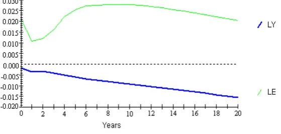
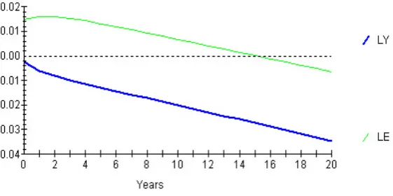
Generalized Impulse Response Function: The generalized impulse response functions trace out responsiveness of the dependent variables in the VAR to shocks to each of the variables. For each variable from each equation separately, a unit shock is applied to the error, and the effects upon the VAR system over time are noted (Brooks (2002)). The results of the impulse response functions are presented in Appendix Figure 2. Some of the significant findings are presented below. For Bangladesh, in response to a unit standard error (SE) shock in output and energy consumption there seems to be very little responses from the counterparts (i.e., from energy consumption and output respectively). In China, in response to the shock in output energy consumption increases more than 10% at the end of 20 years confirming the result of unidirectional causality from output to energy consumption. For India, the results are just the opposite, indicating that at the end of 20th year output goes up to 10% in response to a one S.E. shock in energy consumption. In Malaysia, energy consumption goes down to -20% after 20th year in response to the shock in output while in response to a one S. E. shock in energy consumption output goes up to 12.00% in 20th year. In Pakistan, in response to a shock in energy consumption output decreases more than 15.00% after 20 years. The impulse response functions for Thailand confirms the existence of a unidirectional causality running from output to energy. In response to a shock in output energy consumption increases up to 20.00% level after 20 years. Thus, with a few exceptions the results from impulse response functions also confirm the identified directions of causality for different countries.

5. CONCLUSIONS AND POLICY IMPLICATIONS

(14)

both short-run and long-run Granger causality. Furthermore, generalized variance decompositions and impulse response functions are employed to confirm the robustness of causality tests. The empirical result shows a bi-directional causal link between energy consumption and income in Malaysia for both short-run and long-run. The results further show that there is a unidirectional causality running from output to energy in China and Thailand in the short-run while in the long-run the causality seems to be ceased in case of China. In both India and Pakistan the results indicate the existence of unidirectional causality running from energy consumption to output both in the short-and long-run. Bangladesh proves to be an energy neutral country confirming the fact that it is one of the lowest energy consuming countries in the world. Thus according to the findings of the paper, in Malaysia causality seems to run both ways, in China and Thailand from output to energy consumption, while in India and Pakistan the causality is running from energy consumption to income.

The policy implications for these findings are as follows. For countries like China and Thailand may contribute to the fight against global warming directly implementing energy conservation measures whereas India and Pakistan may focus on technological developments and mitigation policies. For Malaysia a balanced combination of alternative policies seems to be appropriate. Nevertheless, these countries may initiate environmental policies aimed at decreasing energy intensity, increasing energy efficiency, developing a market for emission trading. Moreover, these countries can invest in research and development (R&D) innovate technology that makes alternative energy sources more feasible and thus mitigating pressure in environment.

APPENDIX

Table 1. World Total Energy Consumption by Region, Reference Case, 1990-2030

(Quadrillion Btu) History Projections

Region/Country

1990 2003 2010 2020 2030

Avg. annual % - age change, 2003-2030

OECD

OECD North America 100.8 118.3 131.4 148.4 166.2 1.3

OECD Europe 69.9 78.9 84.4 88.7 94.5 0.7

OECD Asia 26.7 37.1 40.3 44.4 48.0 1.0

Total OECD 197.4 234.3 256.1 281.6 308.8 1.0 Non-OECD

Non-OECD Europe and Eurasia

67.2 48.5 56.5 68.7 79.0 1.8

Non-OECD Asia 47.5 83.1 126.2 172.8 223.6 3.7

[image:14.595.113.486.534.699.2]

(15)

Africa 9.5 13.3 17.7 22.3 26.8 2.6

Central and South America

14.5 21.9 28.2 36.5 45.7 2.8

Total Non-OECD 150.0 186.4 253.6 331.5 412.8 3.0 Total World 347.3 420.7 509.7 613.0 721.6 2.0

Source: Energy Information Administration 2006.

Table 2. Country Profile: Socio-economic and Energy Consumption Fact Sheet (2005)

Indicator(s) Bangladesh China India Malaysia Pakistan Thailand Population, total

(Millions)

153.28 1304.50 1094.58 25.65 155.77 63.00 Population

growth (annual %)

1.81 0.64 1.37 1.82 2.41 0.70

GDP (current US$, Billions)

60.03 2243.85 805.73 136.70 109.50 176.22 GDP growth

(annual %)

5.96 10.40 9.23 5.00 7.67 4.49

Exports of goods and services (% of GDP)

16.58 37.30 20.33 117.64 15.69 73.80

Foreign direct investment, net inflows

(BoP, current US$, Millions)

802.49 79126.73 6676.52 3966.01 2201.00 8048.08

Energy consumption

(quadrillion BTU)

0.693 67.093 16.205 2.546 2.252 3.626

Sources: Data of all the indicators except energy consumption is found from World Development Index by

[image:15.595.112.485.262.529.2]

World Bank while energy consumption data is from Energy Information Administration (EIA).

Table 3. Optimum Lag Length Selection (Schwarz Bayesian Criterion)

[image:15.595.110.486.589.672.2]

(16)

3.2 3.6 4.0 4.4 4.8 5.2 -2.4 -2.0 -1.6 -1.2 -0.8 -0.4 0.0

REFERENCES

Abosedra, S., and H. Baghestani (1989), “New Evidence on the Causal Relationship Between United States Energy Consumption and Gross National Product,” Journal of Energy Development, 14, 285-292.
Al-Iriani, M.A. (2006), “Energy-GDP Relationship Revisited: An Example from GCC Countries Using Panel Causality,” Energy Policy, 34(17), 3342-3350.
Altinay, G., and E. Karagol (2005), “Electricity Consumption and Economic Growth: Evidence from Turkey,” Energy Economics, 27(6), 849-856.
Asafu-Adjaye, J. (2000), “The Relationship Between Energy Consumption, Energy Prices and Economic Growth: Time Series Evidence from Asian Developing Countries,” Energy Economics, 22(6), 615-625.
Brooks, C. (2002), Introductory Econometrics for Finance, Cambridge University Press. Chen, S.-T., H.-I. Kuo, and C.-C. Chen (2007), “The Relationship Between GDP and
Electricity Consumption in 10 Asian Countries,” Energy Policy, 35(4), 2611-2621. Eagle, R.F., and C.W.J. Ganger (1987), “Cointegration and Error Correction
Representation, Estimation and Testing,” Econometrica, 55(1), 26.