Modeling of probe-and-drogue part of an in-flight refueling system

Theses

Thesis/Dissertation Collections

2004

Modeling of probe-and-drogue part of an in-flight

refueling system

Jie Yan

Follow this and additional works at:

http://scholarworks.rit.edu/theses

This Thesis is brought to you for free and open access by the Thesis/Dissertation Collections at RIT Scholar Works. It has been accepted for inclusion in Theses by an authorized administrator of RIT Scholar Works. For more information, please [email protected].

Recommended Citation

By

Jie Van

A Thesis Submitted in Partial Fulfillment of the

Requirement for the

Master of Science

In

Mechanical Engineering

Approved by:

Dr. Agamemnon L. Crassidis

Department of Mechanical Engineering

Dr. Kochersberger, Kevin

Department of Mechanical Engineering

Dr. Kozak, Jeffrey

Department of Mechanical Engineering

Dr. Edward C. Hensel

Department Head of Mechanical Engineering

Agamemnon Crassidis

(Thesis Advisor)

Kevin Kochersberger

Jeffrey Kozak

Title of thesis or dissertation:

Name of author: Degree:

Program: College:

Modeling of Probe-and-Drogue Part of an In-flight Refueling System

Jie Yan

Master of Science

Mechanical Engineering

The Kate Gleason College of Engineering

I understand that I must submit a print copy of my thesis or dissertation to the RIT

Archives, per current RIT guidelines for the completion of my degree. I hereby grant to the Rochester Institute of Technology and its agents the non-exclusive license to archive and make accessible my thesis or dissertation in whole or in part in all forms of media in perpetuity. I retain all other ownership rights to the copyright of the thesis or dissertation. I also retain the right to use in future works (such as articles or books) all or part of this thesis or dissertation.

Print Reproduction Permission Granted:

I, Jie Yan. hereby grant permission to the Rochester Institute of Technology to reproduce my print thesis or dissertation in whole or in part. Any reproduction will not be for commercial use or profit.

Jie Van

S-/If//

mother,

my

Thanks

lot for

Dr.

Agamemnon

L.

Crassidis,

Inthis work, afiniteelementmodelof an in-flightaircraft_refuelingsystemis developed.

The model is a first attempt to describe the dynamics of a probe-and-drogue _refueling

system_commonly used_{by Navy}aircraft. The purpose ofthis workis to_developamodel of the drogue system tobe able to _study control and sensor system requirements for an autonomous _refueling system. This work is intended as a first introduction to an

automated _{in-flight refueling} system with special concentration on the _modeling of a

probe-and-drogue in-flight refuelingsystem foraircrafts. _{An understanding} of whatis an

in-flight refueling system and its significance and influence to the advancement of a

aircraft is first presented. The main character of the system, such as mass, stiffness, damping effect is found from visual observation of an actual drogue system. While

changing these parameters, the responses with different outside forces added on the

1) Abstract

2) TableofContents

3) Abbreviationand

4) ListofFigure

5) ListofTable

1

2

3

4

5

Chapter1 Introductionof_{in-flight refueling}system 6

1. _{What is in-flight refueling}system

2. _Historyand achievements of_{in-flight refueling}system

3. Differenttypesofin-flight refuelingsystem

Chapter 2 _Theory offiniteelement 23

Chapter 3 _Theoryof mathematicalmodel 32

Chapter4 Creationofmathematical model 42

Chapter 5 Discussionand conclusions 75

Chapter6 Reference 92

RAF:

FRL:

RCAF:

BSAA:

FR Inc.:

SAC:

TAC:

NATO:

gpm:

nm:

knot:

Ke:

Me:

M:

K:

C:

E:

i

-Row,j

-column

Royal Air_{Force, UK,}Farnborough

Flight_RefuelingLimited

Royal Canadian Air Force

BritishSouth American Airways

Flight_Refueling,Incorporated-_{FRL American subsidiary}

Strategic Air Command

TacticalAir Command

North Atlantic_TreatyOrganization

gallon per minute

nautical_mile, lnm=6,080 feet

nmperhour

stiffness matrices oftheelement

mass matrixoftheelement

massmatrixofthemathematical modal

stiff matrix ofthemathematical modal

dampingmatrix ofthemathematical modal

Figure 2.1 Beamelements 27

Figure 2.2 Stiffness for beamelement 28

Figure 2.3 Positivesense ofbeam displacement 29

Chapter3

Figure 3.1 Simplificationof probe-and-drogue 32

Figure 3.2 Uniformtwobeamelements

Chapter 4

33

Figure 4. 1 Modeloffree vibration 42

Figure4.2_Forcingfunction fora singlebeamelement 43 Figure 4.3 Beamelementsfor free vibration model 45

Figure 4.4_Gravityon thebeam 46

Figure 4.5 _Gravityonbeamanddrogue 48

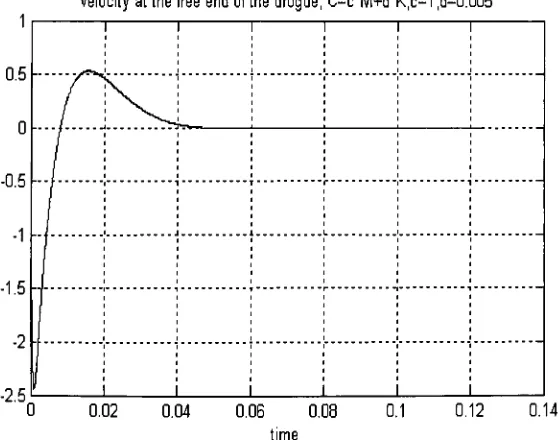
Figure 4.6 Displacementatthefreeend ofthedrogue,c=l,d=0.001 52 Figure 4.7_Velocityatthefreeendofthe_drogue,c=l, d=0.001 52 Figure4.8 Displacementatthefreeendofthe _drogue,c=l,d=0.002 53 Figure4.9 _Velocityatthefreeendofthe_drogue,c=l, d=0.002 54 Figure 4.10 Displacementatthefreeend ofthe _drogue,c=l, d=0.005 55 Figure 4.11 _Velocityatthe freeend ofthe_drogue,c=l, d=0.005 55 Figure 4.12 Displacementatthefreeend ofthe droguewithgravity, c=l, d=0.001 56 Figure4.13 _Velocityatthefreeend ofthedroguewithgravity, c=l,d=0.001 57 Figure 4.14 Displacementatthefreeendofthedroguewithgravity, c=l, d=0.002 57 Figure 4.15 _Velocity atthefreeend ofthedroguewithgravity, c=l, d=0.002 58 Figure4. 16 Displacementatthefreeend ofthe droguewith gravity, c=l,d=0.005 58 Figure4.17_Velocityatthefreeend ofthedroguewith _{gravity, c=l,}d=0.005 59

Figure 4.21 Displacementatthefree end ofthedrogue withoutsideforces,d=0.001 69 Figure4.22_Velocityatthefreeend ofthedroguewithoutside_forces,d=0.001 69 Figure 4.23 Displacementatthefreeendofthedrogue with outside_forces, d=0.002 70 Figure 4.24 _Velocityatthefreeend ofthedroguewithoutside _forces,d=0.002 70 Figure 4.25 Displacementatthe freeendofthedrogue withoutside_forces, d=0.005 71 Figure4.26_Velocityatthefreeend ofthedroguewith outside_forces,d=0.005 71

Chapter 5

Figure 5.1 Displacementatthefreedendofthe_drogue, c=_{0.5 d=0.0005 79}

Figure 5.2 Displacementatthefreedend ofthedrogue, c=_{0.5 d=0.001 79}

Figure 5.3 Displacementatthefreedend ofthe_drogue, c= _{1 d=0.001 80}

Figure 5.4 Displacements at each node 81

Figure5.5 ComparisonofImpulseresponse athigh_frequencydomain 83 Figure5.6ComparisonofImpulseresponse atlow _frequencydomain 84 Figure 5.7 Comparisonofsystemresponse withdifferentmass 88 Figure 5.8 Comparisonof systemresponse withdifferentmass 89

ListofTable

Table4. lUniformtwobeamelements 46

Table 4.2 Matrices offreevibration 47

Table4.3 47

Table 4.4 61

Table 4.5 61

Table4.6 64

What is in-flight refueling

Fuel is required in all aircraft. It's a_{heavy energy} source that consumes space. Fighters

like the F-16 trade _{fuel capacity for} performance and payload. For short-range air

defense, the tradeoff is optimal. _However, to _{fly long} distances, designers resort to

auxiliary fueltanks in various configurations. With rare_exceptions, pilots would choose notto _{carry auxiliary fuel} tanks incombat,whetherfor air-to-air orfor tactical missions. The auxiliary tanks increase fuel consumption, reduce ordinance payloads and tend to

reduce_topspeedoftheaircraft. _Dropping thetanksbeforecombat solvestheseproblems, but the practice is wasteful and involves other compromises. Even with extra _tanks, a

fighter can't cross vast oceans _by the most direct route without _{running dry. The only}

practical answeris topick_upextra_{fuel along}theway.

Day or _night, good weather or _{bad, in-flight refueling keeps military} aircraft in the air,

extending their endurance, range, andpayload and _{vastly increasing} their effectiveness. When _duty calls at the far reaches of the globe, in-flight refueling allows a rapid

achievedthefirstreal_{in-flight refueling}through adangling-hosemethod. Severalmonths

later, another attempt was made. Where aborder-to-border nonstop flight of 1,280 miles

demonstrated how an airplane with a normal range of 275 miles could have its range quadrupled.

What became themuch-publicizedQuestion Markoperation wentforwardwith aFokker C-2A _tri-motor, a _high-wing monoplane of 10,935 _pounds, modified into the receiver.

Two 150-gallon tanks installed in its cabin supplemented its two _{96-gallon wing} tanks. After fuel was received into the cabin tanks it had to be pumped _by hand to the _wing tanks, from where it gravitated to theengines. In _addition, there was a45-gallon reserve

tankfor engine oil. A hatch was cut intheplane's roofto receive the_{refueling hose} and othermaterials. On each side ofits_fuselage,theFokkerwaspaintedwithalarge question markintended toprovoke wonder at how _long the airplane could remain airborne. Two Douglas C-l single-engine _transports, 6,445-pound _biplanes, were transformed into tankers_{by installing}two 150-gallontanks_{for offloading} and a_{refueling hose}that passed through ahatchcutinthe floor. Inthecourse oftheoperation on _1929, thetankers made

forty-three takeoffs and landings. Crews of tankers flew forty-three sorties, twelve of

them at night. _{Altogether, they} delivered 5,660 gallons of fuel (33,960 pounds), 245

gallons of engineoil (1,838 pounds delivered in forty-nine five-galloncans),andstorage batteries, spare _{parts, tools, food, clothing, mail,} and _{congratulatory} telegrams. The Question Mark operation was predicated on its potential _military utility. This

achievement prompted_manypilots to attemptin-flight _refuelingto establish_{long during}

flyingrecord. In_July 1930,therecord was647.5 _{hours,nearly 27 days in}theair.

was _only a trifle betterthan _ninety miles per _hour, and over a distance of 1,000 miles,

most of this speed was lost at fuel stops. But within ten years, aero engine power

quadrupled, which brought more powerful and long-range airplanes, such as Douglas DC-1 andMartin B-10 bomber. So with theelements ofthe modern airplane _{making it}

possible to build _increasing range into an _airplane, people felt no need for the

complication ofin-flightrefueling.

During theWorld War_U, aircraft withlarge internal fuel capacity alleviatedthe needfor

aerial refueling. Atthattime,in-flight refuelingsystemshadsevere drawbacks._However,

changes took place after the Japanese attack on Pearl Harbor brought the United States

into World War _{II, many Americans desperately} wanted to bomb Japan. The most forward U.S. base forsuch an action was Wake _Island, 1,983 miles from_Tokyo, butthe Japanese preempted its use on December _{22, 1941,} when _they overwhelmed its small

garrison of U.S. Marines. In _Washington, Imperial Airways'

use of in-flight refueling

was recalled. The U.S. effort to _develop an in-flight refueling capability went _forward,

although slowly.

It was Sir Alan Cobham andFlight _Refueling Limited _(FRL) the _{company he founded} in 1934 broughtgreat changesto thein-flightrefueling. With World War JJended,FRL's

services were more acceptedthan before. Six surplus Lancasterbombers were obtained

and transformed into tankers and receivers. Each Lancaster tanker would deliver 2,830

U.S. gallons (16,980 pounds). _During the winter of _1946-47, an intensive series of

demonstration flights was flown in association with British South American Airways (BSAA). These were _all-weather, day-and-night operations, and involved distant interceptions that used radar and transponders. Unlike the prewar _refueling that were daylightvisualflightrulesoperations inwhichtankerandreceiver were_rarelyoutofone

another's sight. The object was to simulate mid-ocean rendezvous. FRL used its

nothing extraordinary abouttheoperation.

On Jun _{26, 1946,} the War Department's _Army-Navy Aeronautical Bd agreed

unanimouslythat the nm andtheknot be adopted asstandardunitsofdistanceand speed. With aviation then _"going global"

this made _sense; it brought aviation into

correspondence with geodesic measurements_firmlyin place sincethe eighteenth century.

An nm is the length of one minute of the arc of a meridian at the _Equator, that _is, a

nominal 6,080 feet. A knot is simplya rate of speed: one nm perhour. Thedistance from

Goose _{Bay, Labrador,} the northeastern most air base in North America, to Moscow is

3,106 nm; the distance from New York _City to Moscow is 4,037 nm; and the distance from ChicagotoMoscow is 4,303 nm.

As relations between the United States and the Soviet Union deteriorated after World

War II, U.S. _Army Air Forces'

leaders started _{measuring distances between North}

America and such points in the USSR as _{Magnitogorsk, Novosibirsk, Omsk,} and

Sverdlosk. _They foundthem to be more than a few nautical miles _(nm) too fartofly. A

means of rangeextensionbecameurgent.

In _1948, Air Force contacted with _{FRL, getting} two sets of _{FRL's in-flight refueling} hardware, manufacturing rights toFRL's system and a contract withFRL to produce an additional_{fortyrefueling}sets.

In _1940s, the design of some _{very big} airplanes appeared, such as _Boeing B-52 and

ConvairB-36,B-52was a six-engine _turboprop, with aweightashigh as490,000pounds

and a greatrange 10,860 _{nm,nearly half}the globe's circumference attheequator, while

"carrying fuel to consume fuel". But if applied in-flight refueling _system, the range

reduction would be accepted, and_everything else startedto fall into place. The airplane

wasreducedto_somethingreasonable around300,000pounds.

The bombardment committee _emphatically concluded that the development of in-flight

refueling should be the Air Force's _top priority, not _{only for} the B-52 of the distant

future,but alsofor existing B-29sandthenewB-50s then_enteringtheinventory.

Besides FRL, the other contributor of_{in-flight refueling} system is Boeing. While FRL's

"looped hose"

system dominated the _{in-flight refueling} and its "probe and

drogue"

system was under_{developing, Boeing} invented its _{"Boeing boom",} another _widely used

refueling system. Then in 1958 more and more B-29s were ordered to be modifiedinto

boomtankers,andbecame KB-29Ps. AllofthenewB-50wastobe boomreceivers.

Another significance of _1948, twenty-five years after the world's first aerial _refueling,

was the creation of the world's first in-flight refueling _{unit, the} 43d Air _Refueling

Squadron atDavis-Monthan_{AFB, Arizona,} andthe509th atWalker_{AFB, Roswell,}New

Mexico. At the same _time, FRL created an _{American subsidiary} Flight _Refueling,

Incorporated,knownasFRInc.

On March, 1949, thanks to_{four in-flight refueling using FRL's looped-hose} system on a

KB-29M, the _{first nonstop flight} around the world was made _by a B-50 named _"lucky

ladyJJ" after an unremarkable ninety-fourhours andoneminuteflight.

Promoted_byworld_flight,attheend of _1949,SAC hadsix_refuelingsquadrons and_bythe

end of _1950,thereweretwelvesquadrons withKB-29Ms.

In the fallof _1950, the _{first in-flight refueling} of ajet bombertookplace between a

KB-29Pand aNorth AmericanREM15C assigned to the91st StrategicReconnaissance Wing.

techniques and _{procedures, including} the first night _refueling and instrument weather refueling. _{By 1951,} SAC had _twenty squadrons with a mix ofKB-29Ms and_KB-29Ps, but also two with new _BoeingKC-97s. The next yearit had_{twenty refueling} squadrons with 318tankers. In _1952,SACplannersforthefirsttime incorporated dependenceonin

flight refueling intotheir war_plans, and_{by 1953,} SAC had almost _thirtysquadrons with 502 tankers,most of which were new KC-97s. Attheend of _{1954, SAC's refueling fleet} had grown to thirty-_{two squadrons with 683 tankers, with an average of twenty-one}

airplanes per squadron.

In _1950s, while cold war got_{hot, refueling became} vital. In _{1951, during} Korea war, the

world's firstcombat mission_{using in-flight refueling} was executed. _{This refueling}of_tip tanks to achieve range extension grew beyond occasional operations with probe-tanked

F-80s andRF-80s into Project HIGH _TIDE, in which the three squadrons ofthe 136th Fighter-Bomber _Wingwere equipped with probe tanks. SAC released ten KB-29Ms for

this operation. HIGH TIDE's objective was an operational test of large tactical units,

using in-flight refueling. The project had three phases: _training the three squadrons in a series of small _{exercises, deploying} them in combat air patrol missions over northern Japan,and_deployingthemincombatagainsttargetsin North Korea.

The U.S. Air Forceconcludedfrom HIGH TIDE that, althoughthe_refueling of_tip tanks

was a successful adhocoperation,itwas_only an_emergencysubstituteforareceiver with

a single-point _refueling system. Otherwise, there was no question about in-flight refuelingbeingofvalueto theTactical Air Command_(TAC)andtotheaterairforces.

From _1948, with the assistance of in-flight refueling, flight crossing pacific became

With the development of in-flight _refueling, more demands were submitted to make

refuelingmore efficient and secure. Although thenew B-47 bomberwas a good _sight, it also created problems.

The aircraft was not _wholly compatible with SAC's slower and altitude-limited

piston-engine tankers. _Fully loaded at its 175,000-pound takeoff weight, a KC-97G was hard

puttoreach an altitude of20,000 feet. Buta_{B-47's cruising}altitude was35,000 feet. For its refueling, a B-^17 had to descend to the KC-97's altitude and start _refueling around

18,000feet. Whilethe tankergot _lighter,theB^47 becameheavier, requiringmore speed

to _{stay in} the air than a KC-97's engine could match. The result was the "toboggan"

maneuverin which both airplanes entered a shallow _dive, a _risky descent for two _very large airplanes joined _by a _{refueling boom. Two} airplanes each _weighing more than

150,000 pounds joined _by forty-plus feet of _{ostensibly rigid tubing} do not constitute a

flying machine. _Refuelingcould end as low as 12,000 _feet, after which the B^17 hadto

climbbackto _{its cruising}altitude and consume as much as50percentofthefuel it had justtaken on board. _Clearly, the_{only remedy} was aturbojet tanker thatcould deliver its

offloads at altitudes that turbojet receivers found congenial. On June _1953, KC-97s fulfilledthemissiontorefuelB-47s intheair.

Then with the debut of_B-52, new problem appeared. A KC-97 could servetwo _B-47s,

givingeach a minimum of26,500pounds offuel (22.6percentof aB-47's full load),but

a B-52B's tank required 243,000pounds to fill _it, and a KC-97's total offload (53,000

lbs), was _{only 21} percent of this. In other _words, to achieve _{approximately} the same

delivery given to two B^17s, a minimum of one KC-97 was required for each B-52B.

However, a B-52's fuel consumption was greater than a_B-47's, andtwo KC-97s were

necessary to serve one of the eight-engine giants. _{Additionally,} there remained the incompatibility between turbojet and piston-engine equipment. This not _only required

basing the slow tankers about 1,000 nm ahead of their receivers and _establishing a

KC-97s toguaranteeoneB-52B a minimum26 percent refueling. A tankerlargerthan a

KC-97, one with turbine engines that could cruise at the receiver's speed and altitude

was_clearlyneeded.

The solution wasBoeing's _KC-135, onethe most _widely usedtanker now. A KC-135A

couldlift 31,200 gallons ofJP4 (202,800pounds of aviationjet fuel)_{16,848 gallons in}

wingtanks, 12,178 gallonsin fuselagetanksbelowthecargo_deck, and2,174gallons ina

tankonthe tail cone's upperdeck. In_practice, weightlimitations dictatedabout5percent

lessthan that.Thefuel in its below-decktanks alone was enoughtorefueltwoB^17Es to

33 percent and oneB-52Bto32.5percent.

A KC-135's below-deck fuel tanks,upper-deck and tail cone _tanks, plus its center-wing

tank, allowed it to replenish 57 percent of one B-52B's fuel, or 29 percent of two

B-52Bs'

fuel. Thetankerdidthatat the_{bomber's operating}altitude and_comfortablywithin

itsspeed envelope. Anew_{refueling boom}and_pumpingsystemdelivered JP4toreceivers

atarateof900gpm.

At the end of _1961, the number of SAC tankers peaked at 1,095: 651 KC-97s and 444

KC-135s. This was an "air

force"

unto itself. In addition, the Tactical Air Command

operated about 130 _Boeing KB-50 tankers. The grand total was _{approximately 1,225}

large, multiengine airplanes, all devoted to aerial refueling. The _following year, at the

timeoftheCuban MissileCrisis, SAC'stankersincluded503 KC-97s and515 _KC-135s,

1,018 airplanes fewertotal aircraft,butmorejet KC-135s.

In _1949, North American the AJ-ls became theNavy's first in-flight tankers. Later

AJ-ls were displaced _by improved AJ-2s. After 1956, the AJ-2s were displaced _by the

Douglas A3D, an airplane _{weighing 82,000}pounds and with acombatradius of900nm.

The best aerial tanker the _Navyever hadwas a modification oftheDouglas A3D attack

In _1953,to relievetheNavy's carrier space problem,Douglas developedtheD-704

self-contained

"buddy"

refuelingunit an external store thatheld 300 gallonsof_fuel, a hose-reel _unit, its own _pumping system, and was self-powered _by a generator turned _by ram

air. At first _glance, the unit could be mistaken for an external fuel _tank, but was

distinguished_bythepropellerin itsnosethatturnedits generator.The D-704becamethe

"granddaddy"

of all_buddystores.

Operation HIGH TIDE in Korea proved the overture to the Tactical Air Command's

adoption of aerial refueling. TAC worked out a system for F-lOlCs to operate in pairs. One airplane carried a

"dial-a-yield"

nuclear weapon (ten to _seventy kilotons), and the

other carried abuddy-packtorefuelthe_bomber, whosenormalradiusof690nmcouldbe

extended to 900 nm. TAC submitted the idea of _"every fighter a _{tanker; every fighter} a bomber".

While Air Force focusedon _BoeingB-47,the Britishdevelopedthreebombers of similar weight and performance _{capabilities,} each powered _by four turbojets, the so-called

"V"

bombers the Vickers Valiant, a 140,000-pound airplane of rather conservative _design;

the _delta-wing Avro _{Vulcan, weighing 220,000} pounds; and the _Handley Page _Victor, 216,000 pounds. All had performances similar to the B-47. Later, Valiant and Victor were modified to tanker respectively. The first Victor tankers had two-point refueling,

with an FRL hose-and-drogue unit beneatheach wing. After _1965, later Victors had an additional unit installed beneath their _fuselages, thus _making them three-point tankers. Initially created as _bombers, the Victor tankers _{already had} probes for _receiving; once

converted; they couldboth give and receive. This _{double-duty outfitting} permitted_relay

refueling in which twoor more tankers could_accompany areceiverto give it maximum range, withthetankers_topping off one another. Some yearslater, theVulcans, too, were

convertedfrom bomberstotankers, and_theyalso hadthatdouble-endedcapability. Much later in 1981, the U.S. Air Force first exploited the _versatility of the tanker-receiver_by

In _{1960s, during} warin SoutheastAsia, in-flight refueling tanker, especially KC-135 did

greatachievements. _Byrule ofthumb since _1915,the internal fuel of_{any fighter}plane at

any point in time _{is something less} than 25 percent of its nominal maximum takeoff

weight. Arequirement formore fuel involves strapping on external fuel tanks. Ifthat is notenough,in-flight refueling isnecessary.

In asagaof aerial_refueling,this KC-135 replenishedtwo _{NavyKA-3 tankers,}two_Navy F-8s, and two _{F-4s returning from} the strike, in addition to its F-104s. While it was

pumping fueltoone ofthe_KA-3s, theF-8 fighters came on_{the scene,} desperatefor fuel. The KA-3reeled outits hose forthem. Forafew minutes,aK-135 was_refuelinga

KA-3, which atthe same time was _{refueling F-8s} a tri-levelrefueling. Without the service from this _obliging KC-135, the _Navy airplanes _probably would not have reached their

carrier.

And it was in this war, a KC-135 crew receivedproper credit: the _Mackay Trophy, an

award_dating backto 1912 andgiven forthe most_{extraordinary} aerial flight ofthe year; this wasthefirsttimeatankercrewhadbeen sohonored.

Another extraordinaryworkof_{in-flight refueling}tankerwas _{savingleaking}fighters.

KC-135s occasionally flew leaking fighter planes back to their bases attached to their

refueling booms, meanwhile _pumping enough fuel to _keep the fighter's engine _barely running. The KA-3s didthe same for_Navy fighters and attacked planes, _leading them at

theends oftheir_{refueling hoses.}

In the course ofthe war, KC-135 tankers flew 194,687 sorties, averaging 21,631 sorties per year._Theyexecuted 813,378 in-flightrefueling, an average of90,375 peryear, 7,531

permonth, 251 perday. Total _flyingtimewas 911,364hours, an averageof 10,126 hours

annually, 8,438 hours each month. In total, they delivered almost 1.4 billion gallons of

Atthe same_time,theapplication ofin-flight refuelingtohelicopterenhancedits rescuing capabilitygreatly. From its_inception,the helicopterwas a_severelyrange-limitedaircraft. The _{Sikorsky R-4,} the first operational helicopter of the U.S. _military, was a _charming little machine of2,020 pounds that hadan _operatingradius of _sixty statute miles. In any

vehicle thatlifts its own weight_directlyoffthe earth, weightis worsethancritical it is everything. Fuel is_range,but fuel quicklyadds_uptolots of weight.

Nonetheless, military aviators, fromthe _{very beginning} of _{rotary wing aviation,} viewed thehelicopter as aninstrument torescue people from predicaments with difficultaccess. From thefirstcovertU.S. intervention inthe affairs ofSouth VietnamandLaos in _1962, downed airmen needed rescue. This meant _helicopters, and the effort _quickly grew to

morethanjustrescue. Itmeant _dashingin tosnatchthese airmen outfromundertheguns

of the enemy, _being shot _at, and _{shooting back.} These circumstances generated requirements forrangeextensionand anexpandedloitertime.Helicopter advocatesfaced

thesame problem as theirAircraft andWeapons Boardcounterpartsin 1947: eitherbuild

a _ridiculously large and _hopelessly conspicuous _flying machine, or go to in-flight

refueling.

On December _1965, a CH-3 helicopter and a KC-130 tanker made success in the first

experiment. In that moment, not _{only had} airrescue operations been revolutionized, but alsohadthegeneral scope ofhelicopteroperations.

In the course ofthe war, the helicopters and crews ofthe AirRescue Service picked _up 3,383. It is doubtful that score would have been whatit was without in-flight refueling

extending the range and _{expanding the endurance,} which was _{necessary for} so _many successful executions ofthe mission. The U.S. _{Navy, Marines,} andCoast Guard quickly adoptedin-flight refueling for helicopters built forrescue workand special missions.

Ever since _{then, in-flight refueling nearly} appeared in every major war involved USA.

itneeded an airlift_{capability independent}ofthose_bases, oneitcould_deployunilaterally. In-flight _refueling was the solution. All the while, calls for in-flight refueling services

were increasing. Since then KC-10 appeared, a tanker even more capable than _KC-135, proving US's refuelingcapability.

The KC-10 is a 590,000-pound aircraft with atotal _capacity of 365,000 pounds offuel (56,153 gallons),61 percent ofits takeoff weight, theoretically,all _{deliverable. A wholly}

newboom of McDonnell-Douglas design and_{its pumping} system can delivermore than

1,000gallons per minute. The KC-10A is air_{refuelable, making}possiblerange extension

byrelay, refuelingbya series oftankers. _{Additionally,} someKC-lOs have beenequipped with _{wing-tip refueling} pods with FRL hose-reel systems, _{thereby making} the KC-10A the Air Force's first two-system tanker (boomand_hose), andits first three-point tanker sincetheKB-50s were retiredin 1965.

In 1991, _{during forty-three-day} operation of DESERT STORM, one of the most

interesting things was on _any given _day 18 percent of the airplanes in the air almost

one-fifth oftheforce was tankers.Thetankerswere"first in andlastout".

1.3 Differenttypesof_{in-flight refueling}system

1) Dangle- _and- _grab

system,thefirsteffort ofin-flight refueling_system,

On June 27, 1923, at an altitude of about 500 feet aboveRockwell Fieldon San Diego's North _Island, a hose linked two U.S._Army Air Service airplanes, and one airplane

refueledtheother. _{While only}seventy-five gallons of gasoline were_transferred, theevent

is memorable because it was afirst. Airplanes were de HavillandDH-4Bs, single-engine biplanes of4,600 pounds. 1st Lt. Virgil Hinepiloted the _{tanker; 1st Lt. Frank W. Seifert}

occupied the rear cockpit and handledthe _fueling hose. Capt. Lowell H. Smith flew the

receiver while 1st Lt. John Paul Richter handledthe_{refueling from}therear cockpit.The

refueling system consisted of a fifty-foot length of rubber _hose, trailed from the tanker,

with a_manually operated_{quick-closing} valve at each end. The process is best described

intermsof"you dangleit;I'll grab

it."

Ever since _then, several attempts were made to demonstratethe practical application for

in-flight refueling, and people began to realize how an airplane could have its range

quadrupled. _However, after the first fatal accident happened on November _{18, 1923,} when an airplane was wrecked and a pilot killed while _trying to demonstrate in-flight

refuelingduringan airshow, theexperimentswere dismissedasstunts.

Peoplehadrealizedthatdangleand grabtechnique was_{primitive,clumsy}anddangerous.

It was _necessary to _develop a technique for the _{fueling hookup} that did not demand

unusual_flyingskill.

2) Looped hosesystem

The situation lastedtill L. R. _Atcherly worked out his own in-flight refueling system

-the looped hose system. _{During in-flight refueling} there is a _cruising airplane and a

maneuvering airplane. _Ordinarily, the tanker cruised while the receiver maneuvered to

grabthe hose. _Atcherlyreversed thatorder of work andput almost the whole burden of

the operation on the _tanker, whose crew would _inevitably have more experience with

tankerandthereceiver_trailingcables with grapnels attheirends. While_trailing its_cable, the receiverflew astraight _course, andthe tanker crossed its trackfrom _{behind, trailing} its cable across the receiver's cable until the two grapnels connected. With the two

airplanes nowjoined_by theircables and_{flying side-by-side,} awinch aboardthe receiver

pulledin itscable and_along withitthe tanker'scable. The refueling hosewasattachedto theother end ofthetanker's cable and winchedintothe receiver, where itwasmade fast to a _fueling connection. With the two aircraftjoined _by a huge bight of hose some 300 feetlong,the tankerclimbedtoa position _{slightly higher}than the receivertoputa_gravity headon_{the offload,}valveswereopened, and_{refueling began.}

When refueling was _finished, the receiver disconnected thehose andthe tankerreeledit in, but the two airplanes remainedjoined _by the cables of the original connection. The tanker thenturned away,_breakinga weaklink inthecable connection.

Sir Alan Cobhem brought great changes to the_{in-flight refueling} system. In spite ofthe failure happened before, Cobham was convinced that _{in-flight refueling had} a practical

future. Well aware that the dangle-and-grab _fueling system had no _{future, by} mid-1938 Cobham and the _{company he founded Fight Refueling} Limited _(FRL) had a workable system, which came tobe known as the "loopedhose." Although it was quite similarto what _Atcherly had worked out in the _{early 1930s. FRL's distinct} contribution was the invention and development of the small but vital fittings and hose connections that

transformed _{in-flight refueling from} stunts and experiments to rational flight operations thatcouldbeperformed routinely.

And _later, the idea of single-pint_refueling was introduced. Before _1948, airplanes were refueledmuchlikeautomobiles,exceptthat_bigairplanes hadmore thanonefueltank. At

an airfield, a fuel truck's hose was moved from gas tank to gas _tank, the filler caps

usually locatedon awing's upper surfaceandthefuel flowed_by gravity. Itwas slow and

be at a single point on the airplane into an integrated and well-vented fuel _system, and accomplishedunderpressure.

3) Boeingboom

The cumbersome looped-hose system _{clearly had its limitations,} and the Air Force had asked_Boeingtoinvestigate alternatives. Theresult was the_"Boeing boom". In 1948,the

Boeing Companybegan _testingthe _"Boeingboom" system,consistingof alarge-diameter pipe connectedto the rear of aB-29 andfittedwith small wings atthe end. An _operator, sitting in the tailofthetankeraircraft, controlled theboomto "fly"to areceptaclein the

receiver.The boomwas loweredand

"flown"

to aconnector on thereceiver aircraft.This allowedfuel transfers totakeplace athigherspeeds_and, more_importantly, allowed more

thansix times as muchfuel to flow perminute.FRL's looped-hose system hadan inside diameter of _{only 2.5 inches} and did well to deliver 1 10 gallons per minute (gpm). As most mathematicians and all plumbers _know, if the diameter of pipe is doubled, its capacity is quadrupled. With aninside diameter offour inches and a powerful _pumping

system,theearly-model_Boeingboom delivered 700gallon per minute.

Another important development was the _{"single-point refueling} system"

on receiver

aircraft, which allowed all of an airplane's several fuel tanks to berefilled from a single spotinsteadoffrommultiple nozzles aroundtheairplane.

4) Probe- _and- drogue

system

As early as _1939, FRL's looped hose provided a workablein-flight refueling system for large, multiengine airplanes, but its adaptation to fighter planes in which there was no crew toconnectthehose was_{clearly impossible. Locked into}theideaof_{doingsomething} with a hose, FRL soon hit upon what became known as the probe-and-drogue _system, whereby a small plane was equippedwith a probe thatcouldbe pluggedinto adrogue at

-shaped _drogue, a basket that resembles an oversized shuttlecock. The drogue stabilizes

the _trailing hose and provides a lead into the connector at the end of the hose. The

receiver aircraft is fitted with a probe that extends out from the side ofthe fuselage or

fromthe_leadingedge ofthewing.Thepilot guidestheprobe intothedrogue tomakethe

connection.

On April 1949, the firsttest was given. Air Force flew four B-29s and a pair ofF-84Es

to England for FRL's modification. Two B-29s were given probes that jutted out

conspicuously from the upper curve of the nose of their fuselages, making them

receivers; theseaircraft became known as

"unicorns."

AthirdB-29 was modified with a

singlehose-reelunitin itsfuselageandwithhose-reelunitsinpods,one on each_{wing tip,}

enabling ittorefuel threefighters in a single contact. It wasdesignatedthe YKB-29T;its

three-hose _{capability led} to its _being called the "Triple Nipple." The two F-84Es were

fittedwith single-_point

fuelingsystems.

Later, the idea of _using the new probe- _and

-drogue system to refuel _only the external

drop tanksofthe fighters was introduced. Areceiverprobe andits valve were welded on

theinsideforwardcurvature of an external_droptank. Insteadof_fillingtheinternal_tanks,

the receiver pilot _{simply filled his wing} tanks. _{For straight-wing F-80s} and _F-84Es,

which had wing-tip tanks,subsequentoperations were.

The capacities of the external tanks varied from 160 to 260 gallons (1,040-1,690 _lbs),

andthe movement generated _bya half-ton offuel suddenly placed atthe _{wing tip} could

make an airplane uncontrollable. To avoid _making the airplane unstable in theroll axis,

refuelingthewing-tiptanks of an F-80or anF-84E involvedthree_fuelingcontacts. The

receiver pilot filled his left tank half full, disconnected from the drogue, and connected

with his right tank. When it overflowed, he disconnected that tank and reconnected his

half-full _{left tank, filling} it to an overflow. With both wing tanks _{full, he flew away} to

5) Boom-drogue

-adapter_refuelingsystem

Many hailed probe-and-drogue _refueling as the system of the future. It was _simpler, cheaper, and it weighed less than a_Boeingboom. It imposed less aerodynamic _drag on

the tanker and did not require a skilled operator. But there were also some problems. Probe-and-drogue involvedalotof_rubber, a material thatcouldbecomeunreliablein the

-60F temperatures above30,000 feet. Furthermore it seemed abit toomuchto expect a tiredpilot ofthesluggish mass of a200,000-poundairplanetochasethrough 180degrees

of his vision aheadto put a probe into the small, _dancing target of a drogue's refueling basket. Finally, the optimum transfer _capacity of a probe-and-drogue system was _only 250 gallons per_minute, compared withthe _Boeingboom's 700 gpm. On theother_hand, the receptacle for boom refueling couldbe placed anywhere on the upper surface ofthe

receiver. It couldbeon the fuselage behindthe _canopyor on the_leading edge oftheleft wing. The best position was _{eventually determined} to be outside the pilot's vision, allowingthepilottoconcentrate onthereceiver's position relativetothe tanker.

As a _result, pilots of small maneuverable airplanes liked probe-and- _{drogue; those who} flew_bigairplanes preferredtheboom.

In 1959, theboom's _{incompatibility} with probe-equipped airplanes was resolved with a

boom-drogue-adapter aflexible "tassel" fitted to the end of theboom with a basket at its end to receive a probe. _However, when a boom tanker had an adapter _attached, it

could not servereceiversfittedwithaboomreceptacle.

In _1962, new modifications appeared.Use KB-50 as an_example, in addition tohose-reel

unit in the tanker's tail there was on in a pod at each _wing tip. Each hose-reel unit deployed seventy-five feet of hose. While pumping to three receivers at the same _time,

Chapter2 _Theoryoffiniteelement

2.1 Introductionoffiniteelement

The finite element method is a numerical analysis technique _{for obtaining} approximate

solutions to a wide _variety of _engineering problems. Although originally developed to

study stresses in complex airframe structures, it has since been extended and appliedto

the broad field of continuum mechanics. Because of its _diversity and _flexibility as an analysis_{tool,it is receiving}muchattention in engineeringschools andin industry.

In _reality, either the _geometry or some other feature of the problem is irregular or

"arbitrary". Analytical solutions to problems seldom exist. One possible solution is to

make_simplifying assumptions-_{toignorethedifficulties}

andreducetheproblemtone that

can be handled. Sometimes this procedure _works; but more often than not, it leads to

seriousinaccuraciesor erroneous results. _Now, as computers are_{widelyavailable,} a more

viable alternative is to retain the complexities of the problem and find an approximate

numerical solution.

One ofthe most _widely used numerical analysis methods is finite element method. The

finite element method envisions the solution regions as _{built up} of _many small inter

connected sub-regions or elements. A finite element model of a problem gives a

piecewise approximation to the _governing equations. The basic premise of the finite

element methodis thata solutionregion can be analyticallymodeledor approximated_by

replacing it with an assemblage of discrete elements. Since these elements can be put

2.2 _Theoryoffiniteelement method

In a continuum problem of _{any dimension} the field variable (whether it is pressure,

temperature, displacement, stress or some other _quantity) possesses _{infinitely many}

values because it is a function of each generic point in the _body or solution region.

Consequently, the problem is one with an infinite number of unknowns. The finite

element discretization procedure reduce the problem to one of a finite number of

unknowns _{by dividing} the solution region into elements and_{by expressing} the unknown

field variable in terms of assumed _{approximating function} with each element. The

approximatingfunctions (interpolationfunctions)aredefined intermsofthevalues ofthe

field variables at specified points called nodes. Nodes usually _lay on the element

boundaries where adjacent elements are connected. In addition to _boundary nodes, an

element_mayalsohave afew interiornodes.Thenodal values ofthefieldvariable andthe

interpolation functions for the elements _{completely define} the behavior of the field

variable within theelements. Forthe finite elementrepresentationof a problemthenodal

values ofthe field variable become the unknowns. Once these unknowns are _found, the

interpolationfunctions definethefieldvariablethroughouttheassemblageofelements.

Clearly, the nature of the solution and the degree of approximation depend not _only on

the size andnumberoftheelements usedbutalsoon the interpolationfunctions selected.

However, the functions can't be chose, because certain _{compatibility} conditions should

be satisfied. Often functions are chosen so that the field variable or its derivatives are

continuous across_adjoiningelementboundaries.

Another very important feature of finite element method is the _ability to formulate

solutions for individual elements before _putting them together to represent the entire

problem. This means, we could reduce a complex problem _{by considering} a series of

greatlysimplified problems. Forexample, ifwe are _treating a problem instress _analysis,

we find the force-displacement or stiffness characteristics of each individual element

first, and then assemble the elements to find the stiffness of the whole _structure,

Although using the finite element method, we could approach the formulation of

properties ofindividual elements in differentways; the solutionofa continuum problem

bythefiniteelement method alwaysfollows an_{orderly step-by-step}process asblow:

1. Discretizethecontinuum

This isthe_{first step}to dividethe continuum or solutionregion intoelements. _Duringthis

process, a _variety of element shapes _{may be} used, anddifferent element shapes_{may be}

employedinthesame solutionregion.

2. Select interpolation functions

In this step, we should assign nodes to each element and then choose the interpolation

function to represent the variation of the field variable over the element. The field

variable _{may be} a _scalar, a _vector, or a higher-order tensor. _Often, polynomials are

selected as interpolation functions forthe fieldvariablebecause_they are_easytointegrate

anddifferentiate. The degree ofthepolynomial chosen depends on the number of nodes

assigned _{to the elements, the} nature and number of unknowns at each _node, and certain

continuity requirements imposed at the nodes and _along the element boundaries. The

magnitude of the field variable as well as the magnitude of its _{derivatives may be} the

unknownsatthenodes.

3. Findtheelementproperties

Once thefinite elementmodel has been established, which means once theelements and

their interpolation functions have been selected, we are _ready to determine the matrix

equations_expressingtheproperties oftheindividualelements.

4. _Assemblytheelementpropertiestoobtainthesystem equations

To findtheproperties oftheoverall systemmodeled_bythenetwork of elements we must

"assemble"

all the element properties. In other _word, we combine the matrix equations

the equations for an individual element except _they contain _many more terms because

theyincludeallnodes.

The basis forthe_assembly procedure stems from thefactthat at a_node, where elements

are _{interconnected,} the value of the field variable is the same for each element _sharing

thatnode. Auniquefeatureofthefiniteelement methodisthat_assemblyoftheindividual

element equations generates thesystem equations.

5. Imposethe_boundaryconditions

Before the system equations are_{ready for} solution _they must be modified to account for

the _boundaryconditions oftheproblem. At this stage we impose known nodal values of

thedependentvariables or nodal loads.

6. Solvethesystem equations

The assembly process gives a set of simultaneous equations that we solve to obtain the

unknown nodal values of the problem. If the problem describes steady or equilibrium

behavior then we must solve a set of linear or nonlinear algebraic equations. If the

problemis _{unsteady, the} nodal unknowns are afunctionof_time, and we must solveaset

2.3 Theapplicationoffiniteelement methodto thecase

Inthecaseofthe _{in-flight refueling}system, the systemisconsists of a_long flexiblesteel

hose with an attached drogue at the end. The hose is more than _fifty feet _long and the

outside_{diameter is approximately 2.5}- 3 inches.

Comparing thelength ofthehoseto the

diameter, the diameter is small so that we simulate the probe-and-drogue system as a

flexible beamand createthemathematicalmodel as abeamsystem. _Accordingto thefirst

step of finite element _method, we could discretize the continuum beam system into elements and analyzethebeamelementfirst.

Describebeamelementasbelow:

1

h

w

_

t

Figure 2.1 Beamelements

/:

w:

h:

E:

I:

lengthofbeamelement

width ofbeamelement

heightofbeamelement

Young'smodulus

1 3

moment of_inertia,I= _wh

12

First, the parameters of a beam element, stiffness matrices and mass matrices are

developed. Generally, the relative axial displacements will be small compared to the

lateral displacementsofthebeamelement and canbeassumedtobezero.

Fl,ul

Ml,91

L

F2,u2

)

p 12EI <

r= ru1

r= pu1

M=iiLei

F=^ei

Figure 2.2 Stiffness for beamelement

The local coordinates for the beam element are the lateral displacements and rotation at

the two ends. Each end will have a lateral displacement and a rotation, _{resulting in four}

coordinates, ui, 0i forthefirstendand_U2,02forthe secondend. Thedisplacementcanbe

cpl(x)

91=1

^

1

u2=l cp3(x)

cp4(x)

Figure 2.3 Positivesense ofbeam displacement

The 4X4 stiffness matrix oftheelementisgivenby:

Ke =

EI

12 6/ -12 6/

6/ 4l2 -61

2/2

-12 -61 12 -61

61 2/2 -61

Forthe development of the general equation ofthe_beam, which is a cubic _polynomial,

thedeflection isexpressedintheform

U(X) =

P1+P2+

P3CJ2+P4CJ3

Where

X

= _andPi =_constants

/

Differentiatingyields theslope equation

Z0(x)=

P2+2P3+3P42

The_boundaryconditions are

, = 0 _{at x} = 0 _and , = _{1 at x} = _{/; the}

boundary equations can be expressed _by the

followingmatrixequation:

Ml

101

W2

Wi

10 0 0

0 10 0

1111

0 12 3

Pi

P2

P3

P4

Ifweexpress parameters_{P_bydisplacements,}theequationbecomes:

Pi P2 P3 P4 1 0 0 0 1 0 -2 3 1 -2 0 0 u\ Wi U2 102 2 1-21

Set ui(x) = _{1,9i (x)} = _0,

u2(x) = _{0,02 (x)} =_{0, weobtain a}

groupof constants_P;to define

shapefunctionof_q>i(x);

P, =1,P2=_0,P3=

-3,P4=2;

Thenset_ui(x)=_{0,0i (x)}= _1,

u2(x)=_{0,02 (x)}=0_todefine_<p2(x),get

Pi =_0,P2=/,P3=

-2Z,P4=Z;

Thensetm(x)=_{0,0i (x)}=_0,

u2(x) = _{1, 02 (x)}=0_todefine_<p3(x),get

Pi =

Thenset_ui(x)=_0,0i (x)=_0,

u2(x)=_{0,02 (x)}= 1_{todefine(p4(x), get}

P! =_0,P2=0,P3=

-/,P4=/;

Therefore,the_followingshapefunctionsarederived:

cpi(x) = ₁

3^+2^

(P2(x) =/^-2Z^2+Z^3

(p3(x)= 3^2-2^3

(p4(x)=

Considering the displacement in general to be the superposition of the four shape

functions,i.e.,

y(x)=_{(piui + (p20i+}

(p3u2+ _(p402

= _{q)lql+ (p2q2 + cp3q3 + (p4q4}

The _{kinetic energy}

1 * 2

1 *

T=

Jy

<7 qj

j

2 2 i

1

= _{X X m,y}

qiqj

1 i ;

in which the generalized mass _m^forms the elements ofmass matrix. The my is defined

as

mij =

J0

Thus,themassmatrixoftheelementis a 4X4matrix

156 22Z 54

22/ 4/2

13/

54 13/ 156 -22/

-13/ -22/

4/2 Me

= ml

Chapter3 _Theoryofmathematicalmodel

3.1 _Theoryof mathematical model

The goal of _modeling a probe-and-drogue _{in-flight refueling} system is to analyze the

motion oftheprobe-and-drogue part ofthe system, and understandthe movements, then developa systemforautonomousin-flightrefueling.

As discussed in the chapter _{2, comparing} the diameter of the pipe to the _length, the

diameter is small,so theprobe-and-drogue part ofthe_refuelingsystem canbetreated as a

long and thin flexible steel cantileverbeam. The end ofthe beam is _rigidlyconnectedto

the _tanker,andthepipe will actlike abeam withmoments and lateral_{forces acting}atthe

joints. The relative axial displacements will _{be very} small compared to the lateral

displacements, which couldbeassumedtobezero.

The figure below displaysthesimplifiedmodel ofthe probe-and-drogue system.

Hose

Drogue

Figure 3.1simplificationof probe anddrogue

L: thelengthofthebeam

W: width ofthebeam

H: heightofthebeam

I: areamoment ofinertia= WH

12

In the finite element _method, the continuum beam system is discretized into several

elements to analyze thebeam elementfirst. The assembly ofthe system matrix is found

by superimposing the preceding element matrices. For example, consider a 2-element

VA

c

)

c

Figure 3.2 Uniformtwo-beamelements

Elementa andelementbareidenticalelements exceptforthedisplacementvector.

Elementa: Element b:

ul

02

u3 ul

01

u2

02 03

Wesuperimposethe_preceding matrix of

"a"

withmatrix

"b"

to obtain the _following6 X

Elementa

Elementb

ul

81

u2

92

u3

93

For_example, ifthere are twobeam elements, then the stiffness andmass matrices ofthe

systemis shown asbelow:

iffness matrix

"12 6/ -12 6/

6/ 4/2

-61

2/2

EI

-12 -61 12+12 -61+61 -12 6/

=

Y

2/2

-61+61

4/2+4/2 -61

2/2

-12 -6/ 12 -61

6/ 2/2

-61 Al2

12 6/ -12 6/ 0 0

6/ 4/2 -61

2Z2

0 0

FJ -12 -61 24 0 -12 6/

6/ 2/2

0 8/2 -61 2/2

0 0 -12 -6/ 12 -61

0 0 6/ 2/2

Massmatrb

"156 22/ 54 -13/

22/ 4/2

13/

ml 54

13/ 156+156 -22/+22/ 54 -13/

M=

420 -13/

-22/+22/ 4/2+4/2

13/

54 13/ 156 -22/

-13/ -22/

4/2

ml

420

156 22/ 54 -13/

22/ 4/2 54 13/ -13/ 0 0 0 0 13/ 312 0 0 8/2 54 13/ -13/ 0 0 0 0 54 -13/ 13/ 156 -22/ -22/ 4/2 _

If there are more than _{two elements,} an extension of the matrix in the same manner is

made.Theoverall stiffness and mass matrices ofthe system canthenbe developed.

3.2 Theequation ofmotion

A second-order equationofasystem with viscous_damping and_arbitraryexcitationFcan

bepresentedinmatrixformas:

[m]x+[c]x+[k]x =

[f]

where

[M]:

[K]:

[C]:

mass matrix ofthesystem

stiffness matrix ofthe system

[M] and_[K] aredeterminedbythecharacter ofthesystem.

3.2.1 Freevibration oftheun-damped system

We first discuss free vibration of the un-damped _system, the equation of motion expressed abovebecomes:

[m]x+[k]k =_o

Ifwe_pre-multiplytheequation_byM"1, we getthe_followingterms: M_1M=_{I (unit}

matrix)

M_1K=_{A (asystem}

matrix)

And

IX+AX =0

The system matrix A defines the dynamic properties of the system. _Assuming harmonic

motion

X=-AX and A=_{co2,we get [A-Al][X]}=_0,

Thenthecharacteristic equation ofthesystemis thedeterminantequated_{to zero,}or

[M_1K _Al] = _[A-/l/] =₀

the rootsX_ areeigenvalues, and thenatural frequencies ofthe system are determined_by

the_relationship

Ai=

co2

If substitute Xinto the characteristic _equation, we obtain the _{corresponding} eigenvector

X,andit ispossibletomakeXorthogonal.

3.2.2 ModalmatrixP

Inthe discussion _above, the eigenvalues andeigenvectors ofthe system were developed.

For each _eigenvalue, a _{corresponding} eigenvector exists. The modal matrix for an n

degree-of-freedomsystem_mayappear as

P=

In which,eachXnis acolumnorthogonal vector and_{corresponding}toa systemmode.

ThetransposeofPis

P' =

[X1X2....Xn]'

Ifweformtheproduct ofP'MPand_P'KP, diagonal matrices asbelowaredeveloped:

P'MP = _{[XiXz.^Xd'tM] [XiX2....XJ}

"Ml 0 "

0 M2

in which, the off-diagonal terms are zero because of the orthogonal _property, and the

diagonal termsarethegeneralized massM_.

Similarly,forstiffness matrix_K,

P'KP = _{[XjXz...Xn]'[K] [XxXj....XJ}

~K\ 0

"

0 K2

in_{which, the}diagonalterms arethegeneralizedstiffnessK..

Ifwe divide each column ofP _bythe square root ofgeneralized mass _{M_,} we obtain the

weighted modal matrixP. The diagonal matrix developed from the weighted modal

matrix resultsintheunit matrix

P'M P =1

Since M^K. =Xi

, the stiffness matrix treatedby the weighted modal matrix becomes a

diagonalmatrixoftheeigenvalues

'Ai 0

P'K P =

After development of the eigenvalues, eigenvector and modal matrix, we consider the

equationof motionofan ndegree-of-freedom systemwithviscous _dampingand_arbitrary

excitationF ispresented_bytheform:

[m]x+[c]x+[k]x =

[f]

that _{is generally}a set of n coupled equations.

Aswehavefoundthesolution ofthehomogeneousun-damped equation

[m]x+[k]x =0

which leads to the eigenvalues and eigenvectors that describe the normal modes of the

system and the modal matrix P or P. If we set X = PY, and pre-multiply byP', the

equation abovebecomes:

~p[m ]py+

~p{c]p

T{k^py

~p{f]

in _which, P'MP and P'KP arediagonal matrices. Although in _general, P'CP is not

diagonal,ifCis proportional toMor_K,it isevidentthat P'CP becomes diagonal. Then

thesystemhasproportionaldamping. Theequation of system motionbecomes:

yi+2^iQ)iyt+ca2yi-_ft

we settheproportional_dampingintheformshownbelow:

[C] =_{cc[M] +}P[K]

where a and (3are constants. When different values forparameters a and₃are _chosen, a

new _dampingmatrix _[C] is developed.

Applying theweighted modalmatrix Pto _[C] resultsin

= o/+p

Ai

Az

0 An

= cc/+|3

mi 0

0)1

0 (On

So that

comparingto

it is clearthat

yt+(a+_Pan2)yi+cot2yi= _fi

yt+2^i(ayi+ (a'yi=

fi

2%(Oi=_a+/tot2 _or /fa*2

-2<w+a=0

3.2.4 Statespace version

Convertingtheequation

[m]x+[c]x+[k]x=

[f]

toa state space_model,i.e.,

X=AX+BU

Y=DX _+EU

where X is state _variable, andU is input, if the system is an nth order dynamic system

withminputs, thenX willbean nthorder_vector, Uwillbe anmth vector, Awillbea{n

Xn) matrix,Bwillbe an(n X_m)matrix. If poutputvariables aretobemonitored,Y will

Set

Then

Xi=X

X2=Zi _=x

xi = _xi=x =

[mY[f]-[mY[c]x-[m\x[k]x

=

[mY[f]-[mV[k]xi-[mY[c]x,

XI

X2

0 1 _JXi

[Mr

[a:]

0

[Mr

[F]

Ifwe putforceFintomatrix _[B],and set_[U] as a unit_input,thentheequationbecomes

XI

X2

i Txi

[-[mtiki

0

[mVIf]

[u]

IyMd

X2

+

[E][U]

Ifwe set _[E] matrixtozero and set _[D]matrix as [1 0], then

'Xi'

Xi

61=

&

Ifweset_[D] matrix as [0 1],then

"Xi

M-i,

Analysis above discussed situations where _Xi,X2are single variables. Ifboth _{Xi, X2}are

vectors, with nelements, thenthestate space equation canbemodifiedto:

XI

X2

zeros I

[mT[k]

Xi

Xi +

0

[mV[f]

[u]

Inwhich, zeros is an n Xnmatrix with all elements tobe zero andIis an nXn _identity

Chapter4 Creationofmathematicmodel ofthe_{in-flight refueling}system

4.1 The_Forcingfunction

For the mathematical model of probe-and-drogue part, first consider the free vibration

condition _(i.e.,thereisno _anyoutsideforceadded onthesystem).The only existing force

is the gravity. The longer the pipe, the larger the _{gravity force,} although the _gravity

acceleration is the constant, togeneralize the situation, a_{linearly increasing}force on the

systemis assumed, shownbelow:

Figure 4. 1 Modeloffreevibration

For the equation[m]X+[c]x+[A"]x _{=[p], a} known stiffness and mass matrices of the

system can be _derived, and _{by defining} parameter a and P, the _damping matrix is also

derived, leaving only the force function [F]. According to theory of virtual work of

appliedforce,theshapefunction displacement isexpressedasfollows:

y(x)=_{(piui + cp20i+(p3u2+ cp402}

Thevirtual workoftheapplied_{force gravity}onthebeam is:

8W = \'

p(x)Sy(x)dx

Jo

=Svi

[

Jo Jo Jo JO

where(pi-4(x)are shapefunctionsfora simple_element,shownbelow:

q>i(x)=l 32+23

with =

(p3(x)=₃

42-23

(p4(x)=

x

/

Ifthe same procedure is applied to the end _{forces, Fi, Mi,F2} and_M2,the total virtual

workis represented_by

5W=

Fi8ui+_Mi80 1+F26u2+M2802

Equatingthevirtual work_above, we could obtainthe_{followingrelationship}

Fi =

Jo

jJ

F2 =

Jo

jJ

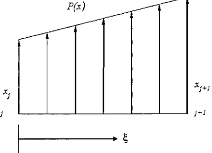
where/ isthelengthof element_{andp(x) is} obtained_{byexaminingFigure4.2,}

P(x) r^*^*,

-"

'

,

V'

i+i

Figure 4.2_Forcingfunctionforasinglebeamelement

p(x)=_(xj+1

-Xj)\+_Xj

The force forthejthnode canbegiven_by

Fj

ljlo[(xj+l -xj)+xj](l-3|2+23)d

Mj

-x.])Z+xj](Z-22+Z3)dZ

, 1 1

M: =1 ( XM+ *,) 1

30 ; 20 J

The force forthe(j+l)thnode canbegiven_by

F,+1 =p(*)p,(*)dfc=

z[(xj+1 -xj)^ +xj](3^2-2^3)^

7 3

Fj+i_J+1 =/( *,-+_ + _*,)

20 ; 20 ;

Mj+l=fop(x)<pi(x)dx=

ljlo[(xi+l -x^+

x^3

-2)^

M;+1,.., =/2( *,.., x,)

20 ; 30 '

The system _forcing function Fi for the ith link can be assembled _{by superimposing} the

proceeding expressions for the general elements. For n nodes (i.e. 1, 2, 3,..., n_+i), the

following are used to obtain the equivalent nodal _force, where we assume the beam is

divided inton elementswithequallength.

7 3 3 7

F(i)=/(

xU)j+l +x{0j)+_{l(xm)j+l +xm)j)}

n+\

11 11

M(t) =

/2(_20*(')y+1 -^X(<->;)+/2(^*0>i);>i + mX<M)

7 3

F(n+_D=

l(x(i)j+l+xU)J)

4.2 Stiffnessand_forcingfunctionmatrices

The beam is divided into several elements. _{For every beamelement, gravity is} the _only

forceapplied onit.

Forthefirstelement

nodel

91.cpQ.Ml

node2

9Q.cp4,M2-l

u2. cp3,F2-2

andforthe second element

node2

02,cp2,M2-2

t>2,<plJ?2-2

node3

93.<p4,M3-l

u3.q>3.F3-l

Figure 4.3 Beamelements for freevibrationmodel

The endingpoint ofthe previous elementis the _starting pointofthe next _element, so for

every node, the generalized force is consisted of two parts, which are derived from

\\f1: shapefunctionof_startingpointoftheelement

\|/2: shapefunctionof_endingpointofthe element

Seetablebelow:

Previouselement _Followingelement

Pl,Vl P1,V2

P2,\|/l P2,\|/2

Table 4.1Uniformtwobeamelements

After the generalized force for each element is _found, we superimpose the previous

elemental forceto thenext one.

Ifwedividethebeamtonelementswithequal length_Z, therearen+1 nodes onthebeam,

Forthefirstnode, thegeneralizedforce isshownbelow:

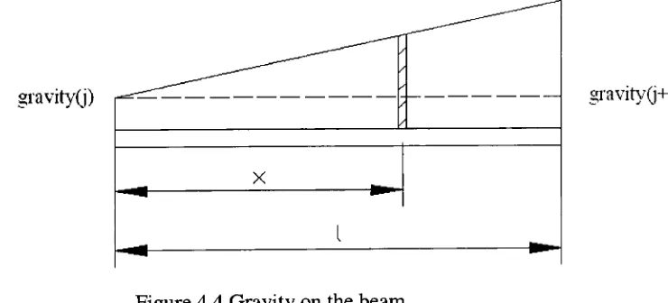
graviry(j)

x

gravity(j+l)

Figure 4.4 _Gravityonthebeam

Set =

, integrate from the starting point to the ending point, at every point, denote

gravity as

Gravityi=_{(gravity (j+1)}

-gravity(j))*

\

F =

f0

jJ

p(/)(f)*IdB, =/

Ifwe divide the beam into n _elements, followed