White Rose Research Online URL for this paper:
http://eprints.whiterose.ac.uk/119374/
Version: Accepted Version
Proceedings Paper:
Khaluf, Y., Markarian, C., Simoens, P. et al. (1 more author) (2017) Scheduling access to
shared space in multi-robot systems. In: Demazeau, Y., Davidsson, P., Bajo, J. and Vale,
Z., (eds.) Advances in Practical Applications of Cyber-Physical Multi-Agent Systems: The
PAAMS Collection. 15th International Conference on Practical Applications of Agents and
Multi-Agent Systems, PAAMS 2017, June 21-23, 2017, Porto, Portugal. Lecture Notes in
Computer Science (10349 ). Springer, Cham , pp. 144-156. ISBN 9783319599298
https://doi.org/10.1007/978-3-319-59930-4_12
[email protected] https://eprints.whiterose.ac.uk/
Reuse
Unless indicated otherwise, fulltext items are protected by copyright with all rights reserved. The copyright exception in section 29 of the Copyright, Designs and Patents Act 1988 allows the making of a single copy solely for the purpose of non-commercial research or private study within the limits of fair dealing. The publisher or other rights-holder may allow further reproduction and re-use of this version - refer to the White Rose Research Online record for this item. Where records identify the publisher as the copyright holder, users can verify any specific terms of use on the publisher’s website.
Takedown
If you consider content in White Rose Research Online to be in breach of UK law, please notify us by
Multi-Robot Systems
Yara Khaluf1, Christine Markarian2, Pieter Simoens1, and Andreagiovanni
Reina3
1
Department of Information Technology, Ghent University, Belgium
2
Department of Computer Science, University of Paderborn, Germany
3
Department of Computer Science, University of Sheffield, S1 4DP, UK
[email protected],[email protected],
[email protected],[email protected]
Abstract. Through this study, we introduce the idea of applying
schedul-ing techniques to allocate spatial resources that are shared among mul-tiple robots moving in a static environment and having temporal con-straints on the arrival time to destinations. To illustrate this idea, we present an exemplified algorithm that plans and assigns a motion path to each robot. The considered problem is particularly challenging be-cause: (i) the robots share the same environment and thus the planner must take into account overlapping paths which cannot happen at the same time; (ii) there are time deadlines thus the planner must deal with temporal constraints; (iii) new requests arrive without a priori knowledge thus the planner must be able to add new paths online and adjust old plans; (iv) the robot motion is subject to noise thus the planner must be reactive to adapt to online changes. We showcase the functioning of the proposed algorithm through a set of agent-based simulations.
1
Introduction
of constraints. The proposed algorithm does not provide the complete solution that can be directly applied to this example but it is a significant step forward in such direction which tackles various challenging aspects.
The considered challenges can be ascribed as the core problems investigated in the two research areas of path planning and scheduling (which we review in Sect. 2). The former area studies solutions to plan the sequence of intermediate locations (configurations) that a robot has to visit (implement) for moving from a starting position to a final destination. Almost every mobile robot system has to deal with this aspect and, in fact, this research area has been very active since a few decades and several solutions have been proposed [3,7]. The latter research area, scheduling, studies how to plan the times of access to shared resources. So-lutions in this area typically aim at problems of sharing computational power [2], while we are not aware of any work that considered the space as the resource that needs to be scheduled for a shared access under deadline constraints. Our work lays at the interface of these two areas; the main idea is to get inspira-tion from soluinspira-tions in scheduling, and employ and adapt them for multi-robot path planning with arrival time deadlines. We illustrate this idea by propos-ing an exemplified time-space planner which we present in Sect. 3. Additional constraints that make the investigated problem more challenging, while closer to a real world application, are (i) stochasticity in robot motion and (ii) on-line requests for new paths. The proposed algorithm is reactive and thus able to modify online the planned paths in response to delays in the robot motion. Additionally, the algorithm evaluates online new requests and either rejects or accepts them. The rejection of a request means that there is no possible plan that would allow reaching the destination within the given deadline without cancelling already scheduled paths. In this case, possible solutions are either to cancel already planned paths, or to extend the temporal deadline. The current version of our algorithm does not make decisions of this type. Instead, when a request is accepted, the planner may modify, if necessary, other planned paths which may include the preemption (i.e., the pausing) of a robot that was moving to allow another robot with a higher priority to access to a spatial resource. We perform a set of agent-based simulations to verify the correctness and efficiency of our algorithm in Sect 4. Finally, we give final remarks on our study in Sect. 5.
2
Related Work
are Dijkstra’s and A∗; and several variants and extensions of these algorithms
have been proposed (e.g.,D∗, or the jump point search) [3,7]. Path planning in
multi-robot systems has been often tackled as an optimization problem focused on finding the shortest collision-free path [1,15,11,16]. Some of these works [1,15] included priorities to give precedence to some robots in case of conflicting ac-cess to space. Differently from other works in multi-robot motion planning, our study takes into account a specific temporal deadline for each robot (thus, for each path) and hence the planner has to schedule movements both in space and in time.
Traditionally, real-time scheduling algorithms have dealt with deterministic execution times such as the worst case execution time [2]. While, stochastic execution times of tasks have been considered only in a limited number of studies. Some of them modified existing deterministic algorithms to support variable execution times, e.g., [10]. Others have implemented heuristic approaches to schedule tasks with stochastic execution times on multi-processors [9]. All these works, similarly to ours, have in common the use of probability distributions to characterize the stochastic execution time of the tasks. In fact, in our study, tasks are not pieces of code to execute (as in traditional scheduling), but tasks are robot motions which are characterized by stochastic execution times. Accounting for time constraints, such as deadlines, in multi-robot systems has been studied only in a limited number of works, e.g., [5,6].
Other works tackled the problem of allocating resources in multiagent sys-temsthrough various methods such as continuous-time MDP and DEC-POMDP—decentralised (partially observable) markov decision processes—e.g. [18], or distributed negotiation protocols, e.g. [8], or metaheuristic approaches, e.g., in vehicle routing [13]. Differently from ours, this class of studies aim to minimize the costs of resource allocation and therefore solve an optimization problem. Instead, we assume specific deadlines for each task and the minimiza-tion of execuminimiza-tion time is not required. Solving a minimizaminimiza-tion problem adds a level of complexity that is unnecessary for our problem; for example, tasks with very far deadlines can make a relaxed use of resources. This difference led us to tackle the problem in a different way, i.e., through a scheduling algorithm. Another class of problems that presents strong similarities with our study is
railway scheduling [14,4] where train journeys with given arrival times are scheduled. As a main difference, our study considers the unpredicted arrival of new tasks which requires to alter the previous schedule and to determine if accepting the new task is possible or not. Additionally, as presented in Sect. 3, we include the notion of link congestion which might allow us to consider the use of resource by entities external to the system under control (e.g. humans).
3
Time-space Planning Algorithm
between two locations can be used by only one robot at a time (even if the other robots move in the opposite or in the same direction, e.g. a lift in a building). We assume a system composed ofN identical robots. A robot may get a taskTi
which is characterized by four attributes: the start timeai,0, the start location,
the destination, and the temporal deadlineDi. This information is not known a
priori but becomes available to the planner only when a new task arrives. In our work we deal with stochastic execution times that can be characterized through its probability distribution.
When a new task arrives, the algorithm evaluates whether to accept or reject it through an acceptance test4. A task passes the acceptance test if (i) a feasi-ble path connecting its start location to its destination is found (space planing) (ii) and if this path can be completed before the deadline expiration and without violating any deadline of previously-scheduled tasks (time planning). Our algo-rithm is reactive to unexpected delays in the robot motion which requires the adjustments of the generated time-space plan. A robot delay is treated as the arrival of a new task using as start location the location where the unexpected delay is reported and as a start time the time at which the robot arrived at that specific location. The acceptance test evaluation is composed of two phases: space planning and time planning. The goal of this study is to illustrate the utility of including a time planning phase—based on scheduling techniques—to allocate spatial resources in a multi-robot system. To highlight and measure the impact of the time planning phase in a clean way, we want to limit as much as possible the influence of arbitrary design choices in the space planning phase, e.g., pos-sible stochastic components. To this end, in the proposed exemplified algorithm we rely on a complete and deterministic planning solution. This choice allows us to illustrate the advantages (and drawbacks) of the time planning phase through a set of experiments on a small size grid environment. In larger environments, this solution would not be viable and the space planning phase can be replaced by any stochastic planning algorithm [3,7].
Space Planning.In this phase, the algorithm finds and orders all feasible paths between the start location and the destination. These paths are ordered by their weight which is computed combining two measures: (i) the length of the path and (ii) the congestion of the links along the path. The path length is a deter-ministic measure that is defined as the sum of the lengths of all links in the path. The congestion of a link is a stochastic measure—characterised by a probability distribution—that represents the number of individuals (including robots and other entities: e.g. humans) that cross the link during a time unit. The conges-tion measure allows the system to operate on more realistic assumpconges-tions with which the robots are not isolated from other systems operating in the same envi-ronment. The algorithm uses the expected value of the congestion distribution. Since we are dealing with known environments, solid distributions for the links
4
congestion can be obtained. These can be time-variant distributions, where the congestion over links varies over time. Our algorithm applies the expected value of the congestion according to the distribution valid during the time of planning. The algorithm combines these two measures (the path length and the path con-gestion) to compute a weightWπj for thej-th pathπj and then order the set of
pathsΠ according to their weights. The weightWπj is computed as:
Wπj =αlπj + (1−α)cπj, (1)
wherelπj is the length measure andcπj is the congestion measure of the pathπj
and αis a design parameter. The lengthlπj is a normalised value in the range
[0,1] computed aslπj =Lπj/M ax(Lπ) withM ax(Lπ) the longest path between
any two locations in the environment (we do not consider loops). Similarly, the congestion cπj is normalised in the range [0,1] as cπj = Cπj/M ax(Cπ) with
M ax(Cπ) the maximum congestion over all paths in the environment. The
com-putation of all feasible paths may be comcom-putationally expensive. We assume a static environment, therefore, the set of pathsΠ can be computed offline for all pairs of start locations and destinations. On the contrary, the congestion measure may possibly vary over time which requires the online computation of weights
Wπj and the online ordering of Π. Additionally, in case a link has a limited
capacity (i.e., a limited number of robots can use a link at the same time), the congestion measure must be updated online each time a new path is planned. In this study, however, we assume that a link has a very limited capacity for robots: it can be used by only one robot at a time. This assumption allows us to simplify the algorithm by ordering Π offline and focusing on the scheduling algorithm to allocate one link at a time to each robot.
Time Planning. During this phase, the algorithm assesses the validity of the paths inΠ sequentially following the ascending order of their weights. The selec-tion of the parameterαdetermines the order of the paths. This parameter has no crucial effect on the performance of the algorithm since we consider an offline average of the link congestion and the goal is not to select the shortest path, but a path that respects the task deadline. The time planning phase algorithm is complete, thus, will evaluate all paths before rejecting a task, therefore, the choice of the parameter α may influence only the algorithm speed. A path is considered valid if it allows the robot to move between the start location and the destination before the task’s deadline is expired and without violating any of the deadlines of already accepted tasks. When a valid pathπj (j is the order of
the path in the setΠ) is found, the task is accepted and the pathπj is assigned
to the task without further checking of the remaining paths inΠ.
Each link in the pathπjrepresents a spatial resource that could be shared among
several tasks that may attempt to access it with time intersections. Hence, we need to schedule the time access to these links. We do so through the widely-used EDF (Earliest Deadline First) scheduling algorithm5. In traditional real-time
5
systems, EDF uses the worst-case execution time to check the task’s schedu-lability and to generate feasible schedules. For multi-robot systems, this is not trivial because of two challenges to overcome: First, the execution time of individ-ual links (i.e., the time spent in crossing a link) is stochastic; Second, scheduling the access to a particular link influences the execution times of all further links used by the related tasks due to new preemptions which were not planned be-fore accessing the link. Therebe-fore, we propose the following approach to facilitate scheduling.
The execution timeρi(h) of a linkhby robotion taskTiis a stochastic measure
that we model using the normal probability distribution. The time is determined by two components: the speed and reliability of the robot resulting in the par-ticular motion time ei of the robot performing Ti, and the congestion on the
link Ch, thus,ρi(h) =ei+Ch. The distribution of ρi(h) can be approximated
by a normal distribution [12] according to the central limit theorem. Hence,
ρi(h) ∼ N(µ, σ),∀i, h. When links have different congestion, the normal
dis-tribution that models the execution time of each links has a different mean and standard deviation, nevertheless, it does not influence the computations of the algorithm. Following the statistical 3-σ rule of the normal distribution, the probability that the execution time of link is smaller thanµ+ 3σis 0.99. Hence, considering the planning valueρi(h) =µ+ 3σallows the system to operate with
the probability of having delays with respect of the planned time on linkh min-imized to 0.01 = 1−0.99. Using this planning value is similar to planning with the worst-case execution time but considering 99% of the cases.
Evaluating the acceptance of pathπjfor taskTiconsists in checking if executing
all linksh∈πj (i.e. moving through them) complies with the deadlineDi and
does not violate the deadlines of the already-scheduled tasks. To make this eval-uation, the algorithm computes for task Ti its ready-to-run timeθi(h) at each
linkh, which is the time at which the robot on taskTiis ready to move through
link h. The expected ready-to-run timeE(θi(h)) on linkhis computed as:
E(θi(h)) =E(ai(h)) +E(γi(h)) (2)
whereE(ai(h)) is the expected arrival time of robotiat linkhandE(γi(h)) is the
expected preemption time of robotibefore executing linkh. The expected arrival timeE(ai(h)) is computed as the sum of the planned times spent in crossing all
the previous linksq∈ {1, . . . , h−1} plus the times spent in preemption on the previous links:
E(ai(h)) =ai,0+
h−1
X
q=1
(ρi(q) +E(γi(q))) (3)
where ai,0 is the start time of task Ti and ρi(q) is the estimated motion time
(e.g., ρi(q) =µ+ 3σ) on linkq.
The expected preemption time E(γi(h)) at link h is calculated as a result of
of the total deadline Di of taskTi:
E(Di(h)) =E(ai(h)) +
lh lπj
×(Di−ai,0) (4)
where lh is the length of link h and lπj is the total length of path πj. After
computing the expected deadline of link h for all tasks that are attempting to access link h with time intersections, EDF assigns them dynamic priorities based on their computed deadlines (i.e., shorter deadline higher priority). After assigning the order in which tasks are allowed to execute link h, it becomes possible to compute the preemption times for the tasks at this link. For taskTi,
this is given by:
E(γi(h)) =E(REs(h)) +
r
X
q=1
ρi(q) (5)
whereREs(h) is the execution time left for taskTs—that was running when task Ti arrived at the linkh— to finish executing linkh. This execution time is zero
when there is no task running over link hwhen task Ti arrives. Furthermore, r is the number of tasks with a higher priority than Ti. After the algorithm
schedules the access to link h and computes the preemption times of all the tasks attempting to access this link, it updates the arrival times of these tasks at all the future links of their planned paths. This update may result in new time intersections which need to be scheduled. While updating the tasks’ preemption times, the algorithm checks, at each link, whether there is any violation of the link deadline Di(h):
E(θi(h)) +ρi(h)≤E(Di(h)) (6)
If a violation appears on at least one of the links, the corresponding path is rejected. Otherwise, it is accepted and assigned to the robot.
Algorithm Complexity. The computations with the highest complexity are performed by the algorithm during the space planning phase in which the al-gorithm iterates over all possible paths between any two nodes. Since we are dealing with known static environments, all these computations are done of-fline, with complexity O(mn2). As mentioned above, we selected a complete
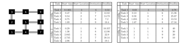
1 2 3 4 5 6 9 8 7
Task Start time Start Location Destination Deadline
co
n
fi
g
.
1 Task 1 0.1465 3 6 0.34
Task 2 0.47 3 7 12.82
Task 3 0.54 2 7 14.73
Task 4 0.75 2 6 7.2
Task 5 1.09 2 9 10.4
co
n
fi
g
.
2 Task 1 0.29 1 8 10.357
Task 2 1.36 3 8 12.90
Task 3 2.045 1 6 22.9
Task 4 2.745 2 7 38.14
Task 5 2.96 3 8 19.1
Task Start time Start Location Destination Deadline
co
n
fi
g
.
3 Task 1 0.03 3 6 0.78
Task 2 0.13 1 6 15.36
Task 3 0.58 3 7 25.67
Task 4 1.055 1 8 13.53
Task 5 1.67 2 8 17.34
co
n
fi
g
.
4 Task 1 1 1 9 40
Task 2 1 1 9 30
Task 3 1 1 9 20
[image:9.595.150.454.113.188.2]Task 4 1 1 9 10
Fig. 1:The environment considered in our scenario and the four configurations used to verify our
algorithm. Tasks marked with light-gray are those not accepted by the algorithm.
4
Results
We performed a set of experiments to validate and showcase the correctness of the proposed algorithm, to prove the utility of having a time planning phase, and to estimate the scalability performance for increasing robot density. We evaluate the algorithm performance in two planning strategies:safeplanning and
risky planning. With safe planning, the algorithm estimates the robot motion execution time (on a link h) as ρi(h) = µ+ 3σ and thus the probability of
missing the planned execution time is only 0.01. Instead with risky planning, the algorithm computesρi(h) =µ+σ and thus the probability of missing the
planned execution time of a link is 0.32. Testing these two strategies allows us to compare the predicted algorithm performances with our simulations’ results. For simplicity, we assume that all links have the same length, and hence their execution times are sampled from a normal distribution with the same meanµ
and standard deviationσ. The parameter αof Eq. (1) for computing the path weight is set to 0.5.
4.1 Validation case studies
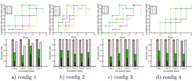
We first start with verifying the correctness and efficacy of the proposed time-space planning algorithm for a multi-robot system of N = 5 identical robots through a set of agent-based simulation experiments. The environment that we consider in our experiments is depicted in Fig. 1, where robots can move between 9 partially connected locations—a small environment increases the chances of concurrent requests for a same link. In our simulations, we model the arrival of tasks using a homogeneous Poisson process with rate of 3 tasks/second. The tasks are generated with random start locations, destinations, start times, and deadlines. The start location is a node that is selected randomly between the nodes on the left side of the grid of Fig. 1 (i.e., either node 1, 2 or 3), while the destination is selected among nodes on the right plus node 6 (i.e., node 6, 7, 8 or 9). The task deadlineDiis randomly selected through a uniform distribution
U(ai,0,3eM) whereeM is the expected execution time of the longest path between
0 1 2 3 4 5 6 Time 1 2 3 4 5 6 7 8 9
Locations along the task path
T 2 T 3 T 4 T 5
Task 2 Task 3 Task 4 Task 5 Accepted tasks 0 0.2 0.4 0.6 0.8 1 Success rate
a) config 1
0 2 4 6 8 10
Time 1 2 3 4 5 6 7 8 9
Locations along the task path
T 1 T 2 T 3 T 4 T 5
Task 1 Task 2 Task 3 Task 4 Task 5 Accepted tasks 0 0.2 0.4 0.6 0.8 1 Success rate
b) config 2
0 1 2 3 4 5 6
Time 1 2 3 4 5 6 7 8 9
Locations along the task path
T 2 T 3 T 4 T 5
Task 2 Task 3 Task 4 Task 5 Accepted tasks 0 0.2 0.4 0.6 0.8 1 Success rate
c) config 3
0 2 4 6 8
Time 1 2 3 4 5 6 7 8 9
Locations along the task path
T 1 T 2 T 3 T 4
Task 1 Task 2 Task 3 Task 4
Accepted tasks 0 0.2 0.4 0.6 0.8 1 Success rate
[image:10.595.143.475.111.250.2]d) config 4
Fig. 2: Results of the agent-based simulations for the four considered task configurations.
(up-per part) Time-space plans generated by the algorithm (safe planning without re-planning). (lower
part) Success rate for 100 simulation runs in three setups.
see the tables in Fig. 1. The plan is generated online while we simulate the task arrival and the robot motion through an agent-based simulator. We execute 100 runs for each configuration and for each planning strategy (i.e., safe and risky). The upper part of Fig. 2 shows the four plans generated by the algorithm (in safe planning with no re-planning). As previously defined, more tasks (i.e., robots) can stay simultaneously on the same node, however, a link can be used by at most a robot at a time. In the plots, solid (horizontal) lines represent a movement on a link departing from that node; the change of node is then visualised as a vertical dashed line of the same color. Preemption (pausing) of a task happens when the horizontal line is missing.
robot does not meet a link deadline, it stops and the task is considered as a failure. These two setups, without re-planning, allow us to match the predicted performances of the algorithm with the agent-based simulation results. In fact, the algorithm that operates in safe planning (i.e., using ρi(h) = µ+ 3σ to
estimate the robot motion execution time) predicts that its plans meets each link deadline more than 99% of the times. Therefore a path that is composed by
klinks is expected to have a success rate of 0.99k. The simulation results match
the predictions: the red bars of Fig. 2(lower part) are always above the respective white overlaying line which marks the lower bound of success. Similarly, the risky planning algorithm (which uses ρi(h) = µ+σ) has 0.32 probability to fail on
each link and, thus, a path composed of k links will succeed with probability greater than 0.68k. Although we see a noticeable decrease in the success rate,
the green bars of Fig. 2(lower part) are always above the predicted lower bound marks (black overlaying lines). The third set of simulations is performed to highlight the role of online re-planning. In this case, we allow the algorithm to re-plan the paths of the tasks which have missed a deadline on a link. While the algorithm operates with a risky planning strategy, we can appreciate that the system performance noticeably increases (compared to the no re-planning case, green bars).
4.2 Effect of time planning
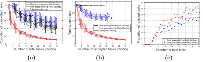
To evaluate the utility of time-scheduling to access shared space, we compared our algorithm with a simple algorithm that assigns to each task its shortest path. Rather than applying time planning, it solves conflicts for accessing shared space resources choosing at random which path to divert (i.e., robots access shared links in arbitrary order). We use µ = 0.7 and σ = 0.3 in all our experiments and we report results for varying number of task requests up to 40. As above, tasks are generated with random start locations, destinations, start times, and deadlines. For each data point, we generate 10 different sets of tasks and we simulate 30 task executions on each plan. The lines connect the average success rate and the vertical bar indicates the standard deviation of the 300 runs. Fig. 3a shows the proportion of completed tasks over the number of requested tasks. For being considered as completed, a task must be first accepted and scheduled by the planner, then the robot must execute the plan and reach the destination before the deadline. Instead, Fig. 3b shows the success rate which is computed as the rate of an accepted task to arrive at destination by its deadline.
0 5 10 15 20 25 30 35 40
Number of total tasks (robots)
0 0.2 0.4 0.6 0.8 1
Proportion of completed tasks
Time-space planning-Safe Strategy Time-space planning-Risky Strategy Only-space planning
(a)
0 5 10 15 20 25 30 35 40
Number of accepted tasks (robots)
0 0.2 0.4 0.6 0.8 1
Task sucess rate
Time-space planning-Safe Strategy Time-space planning-Risky Strategy Only-space planning
(b)
0 5 10 15 20 25 30 35 40
Number of total tasks 0
0.1 0.2 0.3 0.4 0.5 0.6 0.7
Proportion of rejected tasks Time-space planning-Safe StrategyTime-space planning-Risky Strategy
[image:12.595.143.477.115.218.2](c)
Fig. 3:Comparison between time-space planning (both with safe and risky strategy) and the simple
algorithm without time planning phase, in terms of the (a) proportion of completed tasks and (b) task
success rate. (c)Proportion of rejected tasks as a function of total number of requested tasks.
4.3 Scalability on number of tasks
Fig. 3a-c show how, respectively, the proportion of completed tasks, the success rate of a task and the proportion of rejected tasks changes as a function of the number of tasks. The plot of Fig. 3a shows that the risky strategy completes a higher number of tasks in average. This results is due to the fact that the risky planning accepts a larger number of tasks, however presents an higher risk of failure (with a success rate that converges to 0.68, in agreement with the 1-σrule). Differently, the safe planning accepts fewer tasks but assures a higher success rate (around 0.99 according to the 3-σ rule). Additionally, we can see that while the simple algorithm accepts all tasks, the time-space algorithm does not accept anymore tasks above a certain upper bound, visualised through the interrupted lines (around 25 tasks) in Fig. 3b. This upper bound is determined by both the number of tasks (robot density) and the distance between deadlines. The idea behind time-space planning algorithms is to make a decision before the beginning of a task’s execution about the probability of that task to succeed in meeting its deadline. A task begins only if it has a probability of success higher than a certain value, otherwise the task is rejected before beginning. This rejection mechanism has the goal to inform beforehand the user which may look for alternative solutions rather than missing the deadline halfway through.
5
Conclusions
generate plans that respect the given deadlines with predictable performance levels. Natural extensions of this study consists in experimenting the algorithm performance in more challenging setups where each link has different congestion and the system is composed of heterogeneous robots, each with different motion speeds and reliability. Further extensions would consider dynamic environments (with time variant topologies), and larger link capacities.
References
1. Bennewitz, M., Burgard, W., Thrun, S.: Finding and optimizing solvable prior-ity schemes for decoupled path planning techniques for teams of mobile robots. Robotics and autonomous systems 41(2), 89–99 (2002)
2. Buttazzo, G.: Hard real-time computing systems: predictable scheduling algorithms and applications, Real-Time Systems Series, vol. 24. Springer, Berlin (2011) 3. Choset, H.M.: Principles of robot motion: theory, algorithms, and implementation.
MIT Press (2005)
4. Dorfman, M., Medanic, J.: Scheduling trains on a railway network using a discrete event model of railway traffic. Transport. Res. B-Meth 38(1), 81–98 (2004) 5. Khaluf, Y., Birattari, M., Rammig, F.: Probabilistic analysis of long-term swarm
performance under spatial interferences. In: International Conference on Theory and Practice of Natural Computing, pp. 121–132. Springer, Berlin, Germany (2013) 6. Khaluf, Y., Rammig, F.: Task allocation strategy for time-constrained tasks in robot swarms. In: Advances in Artificial Life (ECAL), vol. 12, pp. 737–744 (2013) 7. LaValle, S.M.: Planning algorithms. Cambridge university press (2006)
8. Mailler, R., Lesser, V., Horling, B.: Cooperative negotiation for soft real-time dis-tributed resource allocation. In: Proc. of AAMAS’03. pp. 576–583. ACM (2003) 9. Manolache, S., Eles, P., Peng, Z.: Task mapping and priority assignment for soft
real-time applications under deadline miss ratio constraints. ACM Transactions on Embedded Computing Systems (TECS) 7(2), 19 (2008)
10. Mills, A., Anderson, J.: A stochastic framework for multiprocessor soft real-time scheduling. In: the 16th IEEE Real-Time and Embedded Technology and Appli-cations Symposium. pp. 311–320. IEEE Press (2010)
11. Quottrup, M.M., Bak, T., Zamanabadi, R.I.: Multi-robot planning: a timed au-tomata approach. In: Proc. of ICRA 2004. vol. 5, pp. 4417–4422 (2004)
12. Smith, R., Self, M., Cheeseman, P.: Estimating uncertain spatial relationships in robotics. In: Autonomous robot vehicles, pp. 167–193. Springer (1990)
13. Toklu, N.E., Gambardella, L.M., Montemanni, R.: A multiple ant colony system for a vehicle routing problem with time windows and uncertain travel times. Journal of Traffic and Logistics Engineering 2(1) (2014)
14. T¨ornquist, J., Persson, J.A.: N-tracked railway traffic re-scheduling during distur-bances. Transport. Res. B-Meth 41(3), 342–362 (2007)
15. Van Den Berg, J., Overmars, M.: Prioritized motion planning for multiple robots. In: Proc. of IROS 2005. pp. 430–435. IEEE Press (2005)
16. Wagner, G., Choset, H.: M*: A complete multirobot path planning algorithm with performance bounds. In: Proc. of IROS 2011. pp. 3260–3267 (2011)
17. Wang, C., Savkin, A.V., Clout, R., Nguyen, H.T.: An intelligent robotic hospital bed for safe transportation of critical neurosurgery patients along crowded hospital corridors. IEEE Trans. Neural Syst. Rehabil. Eng. 23(5), 744–754 (2015)