Practical guide to sample size calculations: non-inferiority and equivalence trials

This is a repository copy of

Practical guide to sample size calculations: non-inferiority and

equivalence trials

.

White Rose Research Online URL for this paper:

http://eprints.whiterose.ac.uk/97113/

Version: Accepted Version

Article:

Flight, L. orcid.org/0000-0002-9569-8290 and Julious, S.A. (2016) Practical guide to

sample size calculations: non-inferiority and equivalence trials. Pharmaceutical Statistics,

15 (1). pp. 80-89. ISSN 1539-1604

https://doi.org/10.1002/pst.1716

This is the peer reviewed version of the following article: Flight, L., and Julious, S. A.

(2016) Practical guide to sample size calculations: non-inferiority and equivalence trials.

Pharmaceut. Statist., 15: 80–89. doi: 10.1002/pst.1716., which has been published in final

form at http://dx.doi.org/10.1002/pst.1716. This article may be used for non-commercial

purposes in accordance with Wiley Terms and Conditions for Self-Archiving

(http://olabout.wiley.com/WileyCDA/Section/id-820227.html).

eprints@whiterose.ac.uk https://eprints.whiterose.ac.uk/ Reuse

Unless indicated otherwise, fulltext items are protected by copyright with all rights reserved. The copyright exception in section 29 of the Copyright, Designs and Patents Act 1988 allows the making of a single copy solely for the purpose of non-commercial research or private study within the limits of fair dealing. The publisher or other rights-holder may allow further reproduction and re-use of this version - refer to the White Rose Research Online record for this item. Where records identify the publisher as the copyright holder, users can verify any specific terms of use on the publisher’s website.

Takedown

If you consider content in White Rose Research Online to be in breach of UK law, please notify us by

Practical guide to sample size calculations:

non-inferiority and equivalence trials

Laura Flight1 and Steven. A. Julious1

March 24, 2016

Abstract

A sample size justification is a vital part of any trial design. However, estimating the number of participants required to give a meaningful result is not always straightforward. A number of components are required to facilitate a suitable sample size calculation. In this paper, the steps for conducting sample size calculations for non-inferiority and equivalence trials are summarised. Practical advice and examples are provided that illustrate how to carry out the calculations by hand and using the app SampSize.

1

Introduction

The introduction paper in this series highlighted the key components required to estimate the sample size of a clinical trial [1]. This paper is a practical guide for applying these steps to non-inferiority and equivalence, parallel group clinical trials with a Normally distributed endpoint.

The paper begins by providing a brief explanation of noninferiority and equiv-alence trials in context with their null and alternative hypotheses. Then the formulae for sample size calculations are presented, highlighting the role of each of the components.

Examples are used to demonstrate how this information is used in practice. The examples are illustrated using the app SampSize [2] and also by hand to emphasise the ease of calculating the sample size from the equations provided. Details of how to obtain the app are provided in Table 1.

Table 1: How to obtain the app SampSize The SampSize app is available on the Apple App Store to download for free and can be used on iPod Touch, iPad and iPhones. The app is also available on the Android Market. It requires Android version 2.3.3 and above.

2

Components of a Sample Size

In the introduction to this series, the steps for a sample size calculation are identified. Table 2 gives a summary of these points. An important step before carrying out any sample size calculation is being able to complete this table.

Table 2: Summary of steps required for a sample size calculation

Step Summary

Objective Is the trial aiming to show superiority, non-inferiority or equiva-lence?

Endpoint What endpoint will be used to show the pri-mary outcome? Nor-mal, binary, ordinal or time to event?

Error Type I error: How much chance are you willing to take of rejecting the null when it is actually true?

Type II error: How much chance are you willing to take of not re-jecting the null when it is actually false?

Non-inferiority or equivalence limit What is the minimum clinically acceptable dif-ference?

Population Variance What is the population variability?

Other Do you need to account for dropouts? How many patients meet the inclusion criteria?

3

Non-Inferiority Clinical Trials

treatment is non-inferior. For certain trials, the objective therefore is not to demonstrate that a new treatment is superior to placebo or equivalent to an es-tablished treatment but rather to demonstrate that a given treatment is clinically not inferior or no worse compared with another. The null (H0) and alternative

(H1) hypotheses for non-inferiority trials may take the form as follows:

H0: Treatment A is inferior in terms of the mean responseµA−µB≤ −dN I.

H1: Treatment A is non-inferior in terms of the mean response

µA−µB>−dN I.

The non-inferiority limit,dN I, is defined to be the difference that is clinically

acceptable for us to conclude that there is no difference between treatments. Table 3 summarises how this limit might be selected.

Table 3: Summary of considerations in setting non-inferiority limits. The setting of a non-inferiority limit is a controversial is-sue. Regulatory guidelines exist to provide guidance on the topic [3],[4]. The limit is defined as the largest difference that is clinically acceptable, so that a difference bigger than this would matter in practice [7]. This difference also can-not be greater than the smallest effect size that the active (control) drug would be reliably expected to have compared with placebo in the setting of the planned trial [8].

The definition of an acceptable level of non-inferiority can be made by making a retrospective comparison to placebo such that if we can show that a new treatment is non-inferior to standard treatment, we are indirectly demonstrating that the new treatment is superior to the placebo [9]. In such indirect comparisons, the following ABC needs to be con-sidered [10][11]:

1. The Assay sensitivity of the active control in both the placebo controlled trials and in the active-controlled non-inferiority trial exists.

3. Bias is minimised through steps such as ensuring that the patient population and the primary efficacy endpoint are essentially the same for the placebo-controlled trial and the active-controlled trial.

2. Constancy assumption of the effect of the common com-parator. Such that for two trials in sequence (Trial 1 and Trial 2), the control effect of Treatment B vs placebo in Trial 1 is assumed to be the same as the control effect of Treatment B vs placebo in Trial 2 had placebo been given.

Non-inferiority trials reduce to a simple one-sided hypothesis test. In prac-tice, this is operationally the same as constructing a (1₋2α)100% confidence interval (CI) and concluding non-inferiority provided that the lower end of this CI is greater thandN I.

com-n

r

_r

Z

Z

_d

Type II error ( ) Type I error ( )

Population variance ( 2₎

Non-inferiority Limit (dNI)

Allocation ratio (r)

Difference between mean of treatments A and B

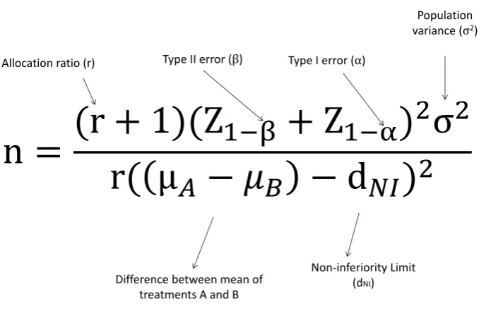
Figure 1: Formula for a non-inferiority parallel group trial.

pare the investigative therapy to an active control. Statistically, they could be considered a special case of equivalence trials. However, they differ in one very important aspect. For a non-inferiority trial, a mean difference a long way from dN I, in a positive sense, is not a negative outcome for the study. While for an

equivalence trial, it would make demonstrating equivalence harder.

The distinction between non-inferiority and equivalence is important. Imag-ine we were designing a role replacement study to assess the work of nurse practitioners against doctors. For an equivalence assessment, we would wish to show that nurse practitioners and doctors are the same with respect to an appropriate clinical outcome, such that simultaneously we would wish to prove that nurse practitioners are as good as doctors and doctors are as good as nurse practitioners. However, with a non-inferiority trial, we would only wish to show that nurse practitioners are as good as doctors. If they are better in other words doctors are worse this would still be a positive outcome.

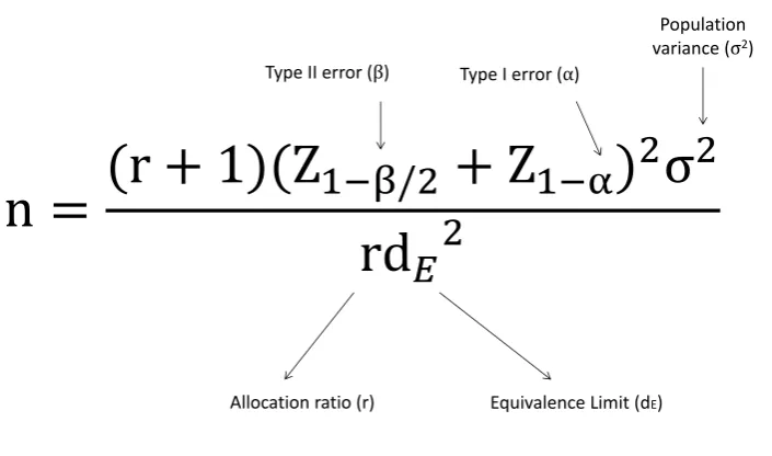
The sample size required for a non-inferiority clinical trial can be calculated using the formula in Figure 1 [5],[6].

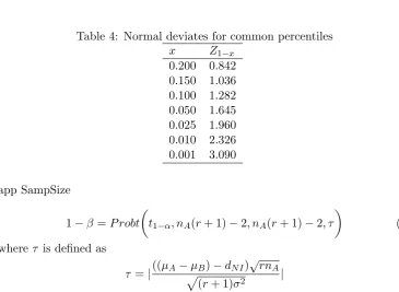
Table 4 gives common Normal deviates for different percentiles. For example, for β = 0.1, we would have x = 0.1 and Z1−x = 1.282, while for α = 0.05, we would havex= 0.025 andZ1−x= 1.96. These values are useful when calculating a sample size by hand.

Table 4: Normal deviates for common percentiles x Z1−x

0.200 0.842 0.150 1.036 0.100 1.282 0.050 1.645 0.025 1.960 0.010 2.326 0.001 3.090 app SampSize

1₋β =P robt

t1−α, nA(r+ 1)−2, nA(r+ 1)−2, τ

(1)

whereτ is defined as

τ =_|((µA−µB)−dN I) √_rn

A

p

(r+ 1)σ2 |

Probt(_·) here is taken from the function in the package SAS (SAS Insti-tute, Inc., Cary , NC, USA). To calculate the sample size, we can use Table 5, which gives calculated sample sizes for various standardised non-inferiority limits (δN I =dN I/σ).

The percentage mean differences are given for the case where it is anticipated that there may be a non-zero difference between treatments, that is,µA−µB 6= 0.

For example, if we had dN I =−10 (arbitrary scale) but we believed there may

be a small difference between treatments, such that µA−µB = 1, then the

percentage mean difference would be 1/10=10%, that is, the percentage of the non-inferiority limit of the mean difference.

Note though the asymmetric effect on the sample size. This is because we only need to show one bound of a 95% CI that has to excludedN I. For the same

example, if we haddN I =−10 (scale arbitrary) but we believed that there may

be a small difference between treatments, such thatµA−µB = 1, then when we

are designing the study, we are anticipating the mean difference to be 11 away from the margin. Therefore, a smaller sample size is needed compared with the assumption ofµA−µB = 0 or µA−µB= 1.

For quick calculations (for 90% power and type I error of 2.5%), the following result can be used [5][6]:

nA=

10.5σ2(r+ 1) ((µA−µB)−dN I)2)

(2)

In the case of r= 1 (2) resolves to:

nA= 21σ

2

((µA−µB)−dN I)2)

(3)

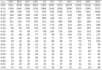
Table 5: Sample sizes (nA) for one arm of a parallel group non-inferiority study

with equal allocation for different standardised non-inferiority limits (δN I =

dN I/σ) and true mean differences (as a percentage of the non-inferiority limit)

for 90% power and type I error rate of 2.5% (from Equation (2)). Percentage mean difference

δN I 25% 20% 15% 10% 5% 0% 5% 10% 15% 20% 25%

Table 6: Rationale for setting a type I error for a non-inferiority trial. The convention for non-inferiority trials is to set the type I error rate at half of that used for a two-sided test used in a superiority trial, i.e. α = 0.025, a type I error rate of 2.5%. It is conventional for one-sided tests to have half the type I error rate of two-sided tests [12].

It could be argued however that setting the type I error rate for non-inferiority trials at half that for superiority trials is consistent. This is because although in a superiority trial we have a two-sided 5% significance level in practice, for most trials, what we have is a one-sided investigation with a 2.5% level of significance. The reason for this is that we have an investigative therapy and a control therapy and it is only the statistical superiority of the investigative therapy that is of interest [9],[13]. It is logical therefore to formulate superiority trials as a one-sided test - which is inevitable. Operationally, statistical assessment of non-inferiority is the same as constructing 95% CI and concluding non-inferiority provided that the lower end of this CI is greater than dN I.

While for a superiority trial, statistical assessment of supe-riority is the same as constructing 95% CI and concluding superiority provided that the lower end of this CI is greater than 0.

3.1 Worked Example

A trial is to be undertaken to investigate the effect of a new pain treatment of rheumatoid arthritis. The trial design being considered is a non-inferiority study. The objective is to show that the new treatment is as good as standard therapy. The primary endpoint will be pain measured on a visual analogue scale. The non-inferiority limit is 2.5mm. The standard deviation is anticipated to be 10mm; assuming a one-sided type I error rate of 2.5% and 90% power. The investigator wishes to estimate the sample size per arm. The true mean difference between the treatments is thought to be zero.

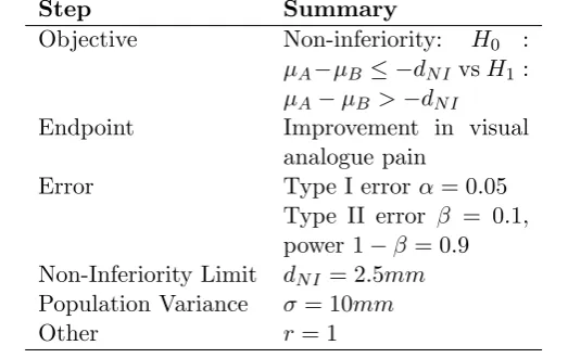
After identifying the key points summarised in Table 7, it is possible to plug the values into the formula in Figure 1. This gives:

nA=

(1 + 1)(Z1−0.1+Z1−0.025)

2₍₁₀2₎

1_×2.52 (4)

Using the percentiles from Table 4, the sample size is calculated to be 336 for each group.

With a non-inferiority limit of 2.5 and a standard deviation of 10 from Table V, the sample size is estimated to be 338 patients per arm.

If we believed that there has to be a small difference of 0.5 between treat-ments, which equates to (0.5/2.5) 20% of the non-inferiority limit, then the sample size could be reduced to 235 patients per arm. The sample size is re-duced as the assumption is that there is a small difference, in favour of the investigative treatment, and so, under this assumption, it should be easier to show non-inferiority.

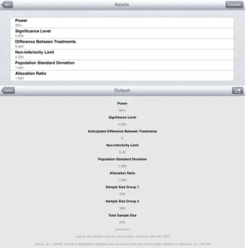
Repeating the calculation with the SampSize app select Non-Inferiority then Parallel Group, Normal and Calculated Sample Size. Example entries and output using standardised entries (standard deviation of 1 and non-inferiority limit of 2.5/10=0.25) are given in Figure 2 using the assumption of a zero difference.

Example entries and output using the original scale of the non-inferiority limits and standard deviation are shown in Figure 3 using the assumption of a 0.5 difference between treatments. Note that a non-inferiority limit of 2.5 and difference of -0.5 equates to the same calculation as a non-inferiority limit of -2.5 and a difference of 0.5.

The SampSize app also gives the sample size as 338 and 235 patients per arm for a difference of 0 and 0.5, respectively, the same as the results from Table 5.

3.2 Superiority Trials Revisited

In a superiority trial, the objective is to determine whether there is evidence of a statistical difference in the comparator of interest between the regimens with reference to the null hypothesis that the regimens are the same.

Table 7: Key components required for sample size for a non-inferiority trial.

Step Summary

Objective Non-inferiority: H0 :

µA−µB≤ −dN I vsH1 :

µA−µB >−dN I

Endpoint Improvement in visual analogue pain

Error Type I errorα= 0.05 Type II error β = 0.1, power 1₋β = 0.9 Non-Inferiority Limit dN I = 2.5mm

Population Variance σ = 10mm

Other r = 1

H0: There is no difference between treatments in terms of the mean response

µA=µB.

H1: A given treatment is superior in terms of the mean response µA > µB.

where in the definition of the null and alternative hypotheses, µA and µB refer

to the mean response on regimens A and B, respectively.

In our discussion, we highlight how, in effect, non-inferiority studies are one-sided tests. The same could be said for superiority trials. However, in our earlier paper, we have used the convention of a two-sided test for superiority. It could be argued this is not strictly correct but it is consistent with International Conference on Harmonisation (ICH) E9 guidelines [12].

3.3 As Good As or Better Trials

For some clinical trials, the objective is to demonstrate that either a given treat-ment is clinically non-inferior or that it is clinically superior when compared with the control, that is, the treatment is as good as or better than the control [5][6][15]. In as good as or better trials, two null and alternative hypotheses are investigated. First, the non-inferiority null and alternative hypotheses:

H0: A given treatment is inferior with respect to the mean response.

H1: The given treatment is non-inferior with respect to the mean response.

If this null hypothesis is rejected, then a second, superiority null hypothesis can be investigated:

H0: The two treatments have equal effect with respect to the mean response.

H1: The two treatments are different with respect to the mean response.

for superiority.

The method used depends on the primary objective of the trial. For example, if the primary objective is to investigate non-inferiority, under the assumption of a small difference between treatments, then the sample size can be calculated for this objective. A calculation can then be made as to what power the study has with the calculated non-inferiority sample size for the superiority objective. Note that in these calculations consideration would need to be made as to the primary analysis population. For a superiority trial, the primary data set may be that is based on an intention to treat (ITT) data set; for a non-inferiority trial, the primary data set may be both the per protocol and the ITT data set [5].

4

Equivalence Trials

In certain cases, the objective of a study is not to demonstrate superiority of one treatment over another but to show that two treatments have no clinically meaningful difference, that is, they are clinically equivalent. The null (H0) and

alternative (H1) hypotheses for such equivalence trials take the form as follows:

H0: There is a clinically meaningful difference between treatments in terms

of the mean response: µA−µB≤ −dE and µA−µB≥ −dE.

H1: There is no clinically meaningful difference between treatments in terms

of the mean response ₋dE < µA−µB < dE.

The equivalence limit dE, equates to the largest difference clinically

accept-able for us to conclude no difference between treatments.

These hypotheses are an example of an intersection-union test, in which the null hypothesis is expressed as a union and the alternative as an intersection [5]. Therefore, to conclude equivalence, we need to reject each component of the null hypothesis.

An approach with equivalence trials is to test each component of the null hypothesis called the two one-sided test (TOST) procedure. In practice, this is operationally the same as constructing a (1₋2α)100% CI and concluding equivalence if the CI falls completely within the interval (₋dE,+dE).

For example, if dE is set to be 10 (arbitrary scale), and after conducting a

trial, a 95% CI for the difference between treatments is found to be (-3, 7). This interval is wholly contained within (-10, 10) so it is possible to conclude that the two treatments are equivalent.

Note that although not covered in this paper, bioequivalence trials are sim-ilar, in an operational sense, to the equivalence trials in terms of the null and alternative hypotheses [5]. The main difference statistically is that the type I er-ror is 5% and 90% CIs are used. There are of course bigger differences clinically in their objectives. The rationale for setting the type I error in an equivalence trials is discussed in Table 8.

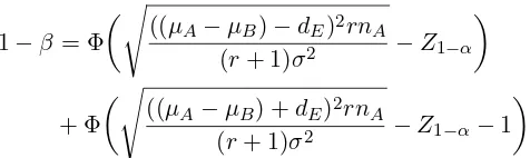
1₋β = Φ

s

((µA−µB)−dE)2rnA

(r+ 1)σ2 −Z1−α

(5)

+ Φ

s

((µA−µB) +dE)2rnA

(r+ 1)σ2 −Z1−α−1

The sample size is then estimated by iterating until the required power is reached. As with inferiority and superiority trials, it is best to use a non-centraltdistribution to calculate the type II error and power. From a non-central tdistribution, the power can be calculated using the following formula [5],[6]

1₋β=P robt ₋t_{1−α,nA(r+1)−2}, nA(r+ 1)−2, τ2

(6) −P robt t_1−α,n

A(r+1)−2, nA(r+ 1)−2, τ1

whereτ1 and τ2 are non-centrality parameters defined as follows

τ1=|

((µA−µB) +dE)√rnA

p

(r+ 1)σ2 |

τ2=|

((µA−µB)−dE)√rnA

p

(r+ 1)σ2 |

Result (6) is used to estimate the sample sizes in Table 9. For the special case of no treatment difference, a direct estimate of the sample size is given in Figure 4.

While under the assumption of a non-central t distribution, the power can be derived from

1₋β = 2P robt ₋t_1−α,n

A(r+1)−2, nA(r+ 1)−2, τ −1

(7)

where τ is defined as

τ = − √_n

ArdE

p

(r+ 1)σ2. (8)

For quick calculations of no treatment difference (for 90% power and type I error rate of 2.5%), the following result can be used

nA=

13σ2_{(r+ 1)}

d2

Er

. (9)

or forr= 1

nA= 26σ

2

d2

E

Table 8: Rationale for setting a type I error for an equivalence trial. Strictly speaking, when undertaking two

simul-taneous one-sided tests, setting α = 0.05 will maintain an overall type I error rate of 5%. How-ever, convention for equivalence trials like for non-inferiority trials described earlier is to set the type I error rate at half of that which would be employed for a two-sided test used in a supe-riority trial, i.e. α = 0.025, a type I error rate of 2.5%.

This is effectively an investigation of two sepa-rate null and alternative hypotheses of the form:

H0:µA−µB ≤ −dE

H1:µA−µB >−dE

and

H0 :µA−µB≥dE

H1 :µA−µB< dE

Table 9: Sample sizes (nA) for one arm of a parallel group equivalence study with

equal allocation for different standardised equivalence limits(as a percentage of the equivalence limit) 90% power and type I error rate of 2.5% (from Equation (6)).

Percentage mean difference

δR 0% 10% 15% 20 25%

Type II error ( ) Type I error ( )

Equivalence Limit (dE)

Allocation ratio (r)

n

r

Z

Z

rd

Population variance ( 2₎

Figure 4: Formula for an equivalence parallel group trial.

4.1 Worked Example

Consider again the trial to investigate the effect of a new pain treatment of rheumatoid arthritis. The objective now is to show that the new treatment is equivalent to a standard therapy. The primary endpoint pain is measured on a visual analogue scale. The largest clinically acceptable effect for which equivalence can be declared is a mean difference of 2.5 mm. The standard deviation is anticipated to be 10 mm; assuming a one-sided type I error of 2.5% and 90% power. The investigator wishes to estimate the sample size per arm. The true mean difference between the treatments is thought to be zero. After identifying these key points summarised in Table 10, it is possible to plug the values into the formula in Figure 4. This gives

nA=

(1 + 1)(Z1−0.1/2+Z1−0.025)

2

1_×2.52 . (11)

Using the common percentiles from Table IV, the sample size is calculated to be 416 for each group. With an equivalence limit of 2.5 and a standard deviation of 10 from Table 9, the sample size is estimated to be 417 patients per arm.

Table 10: Key components required for sample size for an equivalence trial.

Step Summary

Objective Superiority: H0 :µA−µB ≤dE or

H0:µA−µB≥+dE vsH1 :−dE <

µA−µB> dE

Endpoint Improvement in visual analogue pain

Error Type I error α= 0.025

Type II errorβ = 0.1, power 1₋β= 0.9

Equivalence limit dE = 2.5mm

Population standard deviation σ= 10mm

Other r= 1

Repeating the calculation with the SampSize app select Equivalence then Parallel Group, Normal and Sample Size. Example entries and output for the calculation of an equivalence limit of 2.5 and a mean difference of 0.5 are given in Figure 5.

The SampSize app also gives the sample size as 417 and 530 patients per arm for a difference of 0 and 0.5, respectively.

5

Summary

The paper described sample size calculations for trials with a Normally dis-tributed primary endpoint and highlighted how the different non-inferiority and equivalence objectives can impact on calculations. Statistical tables and the app, SampSize, have been used to demonstrate a number of examples of sample size calculations.

While the emphasis of this paper is on trials with a Normally distributed primary endpoint, the principles described can be generally applied to different designs and distributional forms [5],[6].

6

Acknowledgements

Figure 5: Screen shot of SampSize app for equivalence worked example with standardised differences.

References

[1] Flight LG, Julious SA. Practical guide to sample size calculations: an In-troduction.Pharmaceutical Statistics.

[2] epiGenesys. A University of Sheffield company. Available at: https://www.

epigenesys.org.uk/portfolio/sampsize// (accessed 07.07.2015).

[3] CHMP. Guideline on the choice of non-inferiority margin. Doc CPMP/EWP/2158/99 January 2006. Available at: http://www.ema. europa.eu/docs/en_GB/document_library/Scientific_guideline/

2009/09/WC500003636.pdf(accessed 07.07.2015).

[5] Julious SA. Tutorial in Biostatistics: Sample sizes for clinical trials with Normal Data. Statistics in Medicine 2004; 23:192186.

[6] Julious SA. Sample sizes for clinical trials. Chapman and Hall: Bocoa Raton, Florida, 2009.

[7] CPMP. Points to consider on switching between superiority and non-inferiority. (CPMP/EWP/482/99) 27 July 2000. Available at:http: //www.ema.europa.eu/docs/en_GB/document_library/Scientific_

guideline/2009/09/WC500003658.pdf(accessed 07.07.2015).

[8] ICH E10 Choice of control group in clinical trials, 2000. May 2001. Available at: http://www.ich.org/fileadmin/Public_Web_Site/ ICH_Products/Guidelines/Efficacy/E10/Step4/E10_Guideline.pdf

(accessed 07.07.2015).

[9] Jones B, Jarvis P, Lewis JA, Ebbutt AF. Trials to assess equivalence: the importance of rigorous methods.British Medical Journal 1996; 313:3639.

[10] Julious SA. The ABC of non-inferiority margin setting: an investigation of approaches.Pharmaceutical Statistics 2011; 10(5):44853.

[11] Julious SA,Wang SJ, Issues with indirect comparisons in clinical trials par-ticularly with respect to non-inferiority trials. Drug Information Journal

2008; 42(6):62533.

[12] ICH E9. Statistical principals for clinical trials. September 1998. Available at: http://www.ich.org/fileadmin/Public_Web_Site/ICH_

Products/Guidelines/Efficacy/E9/Step4/E9_Guideline.pdf(accessed

07.07.2015).

[13] Bland JM, Altman DG. One- and two-sided tests of significance. British Medical Journal 1994; 309:248.

[14] Flight L, Julious SA. Practical guide to sample size calculations: superiority trials.Pharmaceutical Statistics.