DOI 10.1140/epjc/s10052-016-4065-1 Regular Article - Theoretical Physics
A new method to distinguish hadronically decaying boosted
Z
bosons from
W
bosons using the ATLAS detector
ATLAS Collaboration
CERN, 1211 Geneva 23, Switzerland
Received: 17 September 2015 / Accepted: 8 April 2016
© CERN for the benefit of the ATLAS collaboration 2016. This article is published with open access at Springerlink.com
Abstract The distribution of particles inside hadronic jets produced in the decay of boostedW and Z bosons can be used to discriminate such jets from the continuum back-ground. Given that a jet has been identified as likely result-ing from the hadronic decay of a boostedW or Z boson, this paper presents a technique for further differentiatingZ bosons fromW bosons. The variables used are jet mass, jet charge, and a b-tagging discriminant. A likelihood tagger is constructed from these variables and tested in the simu-lation ofW → W Z for bosons in the transverse momen-tum range 200 GeV< pT < 400 GeV in√s = 8 TeV ppcollisions with the ATLAS detector at the LHC. ForZ -boson tagging efficiencies ofZ = 90, 50, and 10 %, one can achieveW+-boson tagging rejection factors (1/W+) of 1.7, 8.3 and 1000, respectively. It is not possible to measure these efficiencies in the data due to the lack of a pure sample of high pT, hadronically decayingZ bosons. However, the modelling of the tagger inputs for boostedW bosons is stud-ied in data using att¯-enriched sample of events in 20.3 fb−1 of data at√s=8 TeV. The inputs are well modelled within uncertainties, which builds confidence in the expected tagger performance.
1 Introduction
Processes involving the production and decay ofW and Z bosons provide benchmarks for testing the Standard Model (SM), as well as probes of physics beyond the SM (BSM). Since the cross section for the direct strong production of events with multiple jets (QCD multijets) at the Large Hadron Collider (LHC) is much larger than for W and Z boson production, it is usually the case that the leptonic decays of bosons must be used to reduce the overwhelming back-ground. However, when the momentum pV of a bosonV is comparable with its mass,mV, the spatial proximity of the decay products provides a new set of tools that can be
e-mail:atlas.publications@cern.ch
used to distinguish between jets from hadronic boson decays and jets originating from QCD multijet backgrounds. In par-ticular, since the angle between the decay products of a boson V scales with 2mV/pV, for large pV,jet
substruc-turetechniques become powerful tools. This leads to a trade-off between using relatively pure leptonic decays and high-branching-ratio hadronic decays. In some BSM theories, new particles similar toW/Zbosons do not couple directly to lep-tons, so searching for hadronic decays of heavy particles is essential.
Jet substructure techniques developed to distinguish hadronically decaying W and Z bosons from QCD multi-jet background processes have become increasingly sophis-ticated. A recent review is given in Ref. [1]. Both ATLAS [2] and CMS [3] have performed detailed comparisons of the various tagging variables and jet-grooming techniques with the overall conclusion that large QCD multijet suppression factors1are possible while maintaining acceptable levels of boson tagging efficiency. Given aW/Z-boson tagger, a nat-ural next step is to distinguish boson types.
There are several important possible applications of a boson-type tagger at the LHC. First, a type tagger could enhance the SM physics program withW andZ bosons in the final state. Measurements of this kind include the deter-mination of the cross sections forV+jets,V V, andtt¯+V. Another important use of a boson-type tagger is in searches for flavour-changing neutral currents (FCNC). Due to the Glashow–Iliopoulos–Maiani (GIM) mechanism [4], FCNC processes in the SM are highly suppressed. Many models of new physics predict large enhancements to such pro-cesses. Both ATLAS and CMS have performed searches for FCNC [5,6] of the formt→ Z qin the leptonic channels, but these could be extended by utilizing the hadronic Z decays as well. FCNC processes mediated by a leptophobicZsuch ast → Zqmay be detected only via hadronic type-tagging methods. A third use of a boson-type tagger is to catego-rize the properties of new physics, if discovered at the LHC.
For instance, if a new boson were discovered as a hadronic resonance, a boson-type tagger could potentially distinguish aW(→ qq)from a Z(→ qq) (where mass alone may not be useful). This is especially relevant for leptophobic new bosons, which could not be distinguished using leptonic decays.
Labelling jets as originating from aW orZ boson is less ambiguous than quark/gluon labelling. AW boson can radi-ate aZ boson, just like a quark can radiate a gluon, but this is heavily suppressed for the former and not for the latter. The radiation pattern of jets fromW- and Z-bosons is less topology dependent because it is largely independent of the other radiation in the event asW andZ bosons are colour singlets. Aside from the production cross section and subtle differences in differential decay distributions, the only fea-tures that distinguish betweenWandZbosons are their mass, charge, and branching ratios. Experimentally, this means that the only variables that are useful in discriminating between hadronic decays of W and Z bosons are those which are sensitive to these properties. The three variables used in the analysis presented here arejet mass, sensitive to the boson mass,jet charge, sensitive to the boson charge, and a b-taggingdiscriminant which is sensitive to the heavy-flavour decay branching fractions of the bosons. The application of a boson-type tagger in practice will be accompanied by the prior use of a boson tagger (to reject QCD multijet processes). The type-tagger variables are largely independent of typical boson-tagger discriminants liken-subjettiness [7], which rely on the two-prong hard structure of both theWandZdecays.2 This paper introduces a jet tagging method to distinguish between hadronically decayW and Z bosons at the LHC, and documents its performance with the ATLAS detector at√s = 8 TeV. The paper is organized as follows. Sec-tion2describes the simulated datasets used in constructing and evaluating the boson-type tagger. Following a discussion of the differences between the properties ofWandZbosons in Sect.3, Sect.4defines the three discriminating variables. The construction and performance of the tagger are detailed in Sect.5 and the sensitivity to systematic uncertainties is described in Sect. 6. The input variables are studied in a dataset enriched in boostedW bosons in Sect.7. The paper ends with a discussion of possible uses of the tagger in Sect.8
and conclusions in Sect.9.
2 Datasets
Two sets of Monte Carlo (MC) simulations are generated, one to study the tagger’sW versusZperformance and the other to compare the tagger inputs forW bosons with the data. Simulations of hypotheticalW → W Z production and
2See Sect.A.for details.
decay provide a copious source of boostedW andZ bosons whose pT scale is set by the mass of theW boson. Such events are used to construct a tagger to separate hadronically decaying boostedW andZ bosons, as well as to evaluate its performance. It is not possible to measure the performance directly in the data due to the lack of a pure sample of boosted, hadronically decaying Z bosons, but the modelling of the tagger inputs can be studied using hadronically decayingW bosons fromtt¯events in the data.
A simulated sample of W bosons is generated with PYTHIA8.160 [8] using the leading-order parton distribu-tion funcdistribu-tion set (PDF)MSTW2008[9,10] and theAU2[11] set of tunable parameters (tune) for the underlying event. The baseline samples use PYTHIAfor the 2 → 2 matrix ele-ment calculation, as well aspT-ordered parton showers [12] and the Lund string model [13] for hadronization. Additional samples are produced with HERWIG++ [14], which uses angular ordering of the parton showers [15], a cluster model for hadronization [16], as well as theEE3[17] underlying-event tune. TheW’ differs from the SMW boson only in its mass and the branching ratioW→W Zis set to 100 %. The WandZbosons are produced with a mixture of polarizations, but the longitudinal polarization state dominates because mW,mZ mW. In order to remove artifacts in the pT dis-tributions of theWandZbosons due to the generation ofW particles with discrete masses, thepVTspectra are re-weighted to be uniform in the range 200 GeV< pTV <400 GeV. As is discussed in Sect.1, for pT >200 GeV, a jet with large radius is expected to capture most of theWorZboson decay products. The range is truncated to pT<400 GeV because hadronically decayingW bosons can be probed with data in this pTrange; there are too few events in the 8 TeV dataset for pT>400 GeV.
Top-quark pair production is simulated using the next-to-leading-order (NLO) generatorPOWHEG-BOX[18–20] with the NLO PDF set CT10[10] and parton showering from PYTHIA 6 [21]. The single-top (s-,t-, and W t-channel) backgrounds are modelled withPOWHEG-BOXandPYTHIA 6, as for the nominaltt¯simulation. The PDF setCT10f4[9] is used for thet-channel and CT10is used for thes- and W t-channels. For theW t−channel, the ‘inclusive Diagram Removal’ (DR) scheme is used for overlap withtt¯[22]. The W+jets andZ+jets backgrounds are modelled withALPGEN 2.1.4[23],PYTHIA 6and theCTEQ6L1PDF set [24]. Dibosons are generated withHERWIG 6.520.2[25] using the CTEQ6L1 PDF set and the AUET2 tune [26]. Ver-sion 6.426 is used everywhere for PYTHIA 6, with the Perugia2011Ctune [27].
2012 run. The effects of pileup are modelled by adding multi-ple minimum-bias events, which are simulated withPYTHIA 8.160, to the generated hard-scatter events. The distribution of the number of interactions is then weighted to reflect the pileup distribution in the 2012 data. A sample ofW bosons is selected from data taken in 2012 at centre-of-mass energy of√s=8 TeV fromtt¯candidates as described in Sect.7.
3 Distinguishing aZboson from aW boson
Decays ofW or Z bosons are characterized by the boson’s mass and coupling to fermions. The mass difference between theW andZ boson is about 10 GeV and if produced from a hard scatter or the decay of a heavy enough resonance, both bosons are produced nearly on-shell since the width
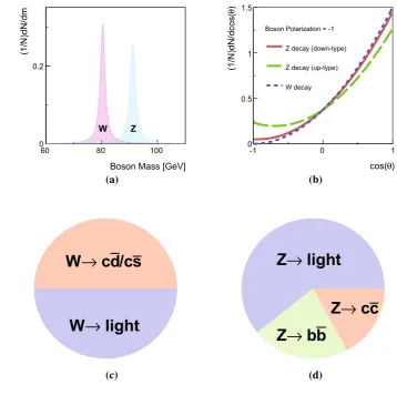
V =2.1 (2.5) GeV is much less than the massmV =80.4 (91.2) GeV forW (Z) bosons [30]. The Breit–Wigner res-onance curves for W and Z bosons are shown in Fig. 1a. The separation between the curves is a theoretical limit on how well mass-sensitive variables can distinguish between W and Z bosons. For hadronic boson decays, the mass peaks measured with jets are broader. This is because the jet-clustering algorithm for final-state hadrons loses
parti-cles at large angles to the jet axis and includes extra partiparti-cles from the underlying event and pileup.
The generic coupling of a bosonV to fermions is given bygVγμ[cV−cAγ5], wheregVis a boson-dependent over-all coupling strength, and cV and cA are the vector and axial-vector couplings, respectively. The W boson couples only to left-handed fermions socV = cA =1 withgW ∝
[image:3.595.186.545.370.726.2]k NCGFm3W|Vi j|2, where GF is the Fermi coupling con-stant,Vi jis a Cabibbo–Kobayashi–Maskawa (CKM) matrix element [31,32],krepresents higher-order corrections, and NC=3 for the three colours of quarks andNC=1 for lep-tons. The CKM matrix is nearly diagonal soW+→ud¯and W+→cs¯are the dominant decay modes. Small off-diagonal elements contribute to the other possible decay modes, and the overall hadronic branching ratios are approximately 50 % forW → c X and 50 % forW →light-quark pairs. TheW boson has electric charge±1 in units of the electron charge, so by conservation of charge, its decay products have the same net charge. The scalar sum of the charge of all the final-state hadrons originating from aW boson decay is not infrared safe (directly sensitive to the non-zero detection threshold), so there are limits to the performance of charge tagging dictated by the energy threshold placed on charged particles in the event reconstruction.
Fig. 1 aBreit–Wigner resonances for theW(red) and Z(blue) bosons,bangular distribution of the decay products of transversely polarizedW/Zbosons with respect to the spin direction in the boson rest frame,chadronic branching fractions of theW+ boson, anddof theZboson. In c,d,lightstands for decay modes not involvingb,cquarks
Boson Mass [GeV]
(1/N)dN/dm
0 0.2
W Z
) θ cos(
60 80 100 -1 0 1
)
θ
(1/N)dN/dcos(
0 0.5 1 1.5
Boson Polarization = -1
Z decay (down-type)
Z decay (up-type)
W decay
light
→
W
s
/c
d
c
→
W
Z
→
light
c
c
→
Z
b
b
→
Z
(b) (a)
In contrast toWboson decays,Zbosons decay to both the left- and right-handed fermions. The partial width forZ → f f¯is proportional tok NCGFm3Z[c2V+c2A]. The factorscV andcAare slightly different for up- and down-type fermions. Thebb¯branching ratio is 22 %, thecc¯branching ratio is 17 % and the sum of the remaining branching ratios is 61 %.W boson decays tob-quarks are highly suppressed by the small CKM matrix elementsVcb and Vub, so that identifying b -hadron decays associated with a -hadronically decaying boson is a powerful discriminating tool. Branching ratios are plotted in Fig. 1d for Z decays to light quarks, c-quarks, and b -quarks, and in Fig.1c for theWboson decays to light quarks andc-quarks.
Since the coupling structure is not identical forW and Z bosons, the total decay rates differ, and the angular dis-tributions of the decay products also differ slightly. How-ever, even at parton level without any combinatoric noise, the differences in the angular distributions are subtle. There is no difference for the two bosons with longitudinal polar-ization because the distributions for right- and left-handed fermions are the same. The distributions are different for right- and left-handed fermions for transversely polarizedW and Z bosons, as shown in Fig.1b. The relative contribu-tion of left- and right-handed components for theZ decays depends on the quark flavour; for up-type quarks the rela-tive contribution from right-handed fermions is 15 % while it is only 3 % for down-type quarks. Intt¯decays, the fraction of longitudinally polarizedW bosons (ignoring theb-quark mass) is m2t/(m2t +2m2W) ∼ 0.7. In contrast, the boson is mostly transversely polarized in inclusiveV+jets events. Any discrimination shown in Fig.1b is diluted by the longi-tudinal polarization, combinatorics, non-perturbative effects, and detector reconstruction, so angular distributions are not considered further in this paper.3
4 Definitions of reconstructed objects
ATLAS is a multi-purpose particle detector [33] with nearly 4π coverage in solid angle.4 The energy of the hadronic
3The impact of polarization on distinguishing boostedW boson jets from QCD multijets has been studied in Ref. [3]. There are small dif-ferences in performance between transversely and longitudinally polar-ized bosons, but any differences are less relevant forWversusZtagging where the angular distributions are identical for longitudinally polarized bosons and only slightly differ for transversely polarized bosons. 4 ATLAS uses a right-handed coordinate system with its origin at the nominal interaction point (IP) in the centre of the detector and thez-axis along the beam pipe. Thex-axis points from the IP to the centre of the LHC ring, and they-axis points upward. Polar coordinates(r, φ)are used in the transverse plane,φbeing the azimuthal angle around the beam pipe. The pseudorapidity is defined in terms of the polar angleθ asη= −ln tan(θ/2). Transverse momentum and energy are defined in thex–yplane aspT=p·sin(θ)andET=E·sin(θ).
decay products of boosted bosons is measured by a system of calorimeters. The electromagnetic calorimeter consists of a Pb/liquid-argon sampling calorimeter split into barrel (|η|
<1.5) and endcap (1.5<|η|<3.2) sections. The hadronic calorimetry is provided by a barrel steel/scintillating-tile calorimeter (|η| < 1.7) and two endcap Cu/liquid-argon sections (1.5 < |η| < 3.2). Finally, the forward region (3.1 < |η| < 4.9) is covered by a liquid-argon calorime-ter with Cu (W) absorber in the electromagnetic (hadronic) section. Energy depositions are grouped into topological calorimeter-cell clusters [34] and then calibrated using the local cluster weighting algorithm [35,36]. Jets are formed from clusters using two different jet algorithms.Small-radius jetsare built with the anti-ktalgorithm with jet radius param-eter R = 0.4 [37].Large-radius jetsare formed using the anti-kt algorithm with R = 1.0 and then trimmed [38] by re-clustering the jet constituents with thektalgorithm using
R = 0.3 and removing the constituents with pT less than 5 % of the original jet pT. Both the small- and large-radius jets are further calibrated to account for the residual detec-tor response effects. For small-radius jets, this is a pT- and
η-dependent energy calibration, plus a correction to mitigate the contribution from additional pp collisions and to sup-press jets from these additional collisions [39]. In addition to pT- andη-dependent energy corrections, large-radius jets J have a calibratedjet mass:
m2J =
j∈J
Ej 2
− j∈J
pj 2
, (1)
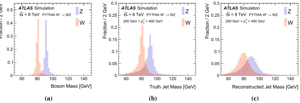
where Ej is the energy of cluster j andpj is a vector with magnitude Ej and direction(φj, ηj). The jet mass calibra-tion depends on the calibrated jet energy and on the jetη[45]. When aWorZboson is produced with large enough momen-tum, its decay products are collimated. When 2mV/pV ∼1, an R = 1.0 trimmed jet captures a large fraction of the decay products and the jet-mass scale is set bymV. Since theW and Z boson masses differ by about 10 GeV, the jet mass can be used to discriminate between these two parti-cles. The distributions of the boson masses and jet masses for hadronically decayingW andZbosons are shown in Fig.2. The particle-level (‘truth’) jet mass is constructed from sta-ble particles in the MC simulation (cτ > 10 mm), exclud-ing neutrinos and muons, clustered with the same jet algo-rithm as for calorimeter-cell clusters. The QCD processes that govern the formation of stable particles from theW and Z decay products create a broad distribution of jet masses even without taking into account detector resolution. Con-structing the jet mass from calorimeter-cell clusters further broadens the distribution. The jet-mass resolution (physical
Boson Mass [GeV]
60 80 100 120 140
Fraction / 2 GeV
0 0.1 0.2 0.3 0.4
0.5 ATLASSimulation
WZ → PYTHIA W'
= 8 TeV
s Z
W
(
a
)
Truth Jet Mass [GeV]
60 80 100 120 140
Fraction / 2 GeV
0 0.05 0.1 0.15 0.2 0.25 0.3 ATLASSimulation WZ → PYTHIA W'
= 8 TeV s
< 400 GeV V T 200 GeV < p
Z
W
(b)
Reconstructed Jet Mass [GeV]
60 80 100 120 140
Fraction / 2 GeV
0 0.05 0.1 0.15 0.2 0.25 0.3 ATLASSimulation WZ → PYTHIA W'
= 8 TeV s
< 400 GeV V T 200 GeV < p
Z
W
[image:5.595.57.544.55.223.2](c)
Fig. 2 aThe boson mass at generator level,b‘truth’ jet mass (at particle level) after parton fragmentation, andcreconstructed jet mass distributions. Theleft plothas a different vertical scale than theright two plotsand also has nopTrequirement
masses. For example, the standard deviation of the detec-tor resolutionσ(mreco jet/mtruth jet)is approximately 10 %. The jet-mass variable nevertheless has some discriminating power.
The momentum and electric charge of particles travers-ing the detector contain information about the charge of their parent boson. The tracks of charged particles are measured in a 2 T axial field generated by a solenoid magnet which surrounds the inner detector (ID) consisting of silicon pix-els, silicon micro-strips, and a transition radiation tracking detector. Charged-particle tracks are reconstructed from all three ID technologies with a full coverage inφ,|η|<2.5 and pT>400 MeV. The chargeqof a track is determined as part of the reconstruction procedure, which uses a fit with five parameters: the transverse and longitudinal impact param-eters,φ,θ,andq/p, where p is the track momentum. To suppress the impact of pileup, tracks are required to origi-nate from the primary collision vertex, which is defined as the vertex with the largestpT2computed from associated tracks. Additionally, tracks must satisfy a very loose quality criterion for the track fitχ2per degree of freedom, which must be less than three. Tracks are associated with jets using ghost association [40]. The charge of tracks associated with a jet is sensitive to the charge of the initiating parton. In order to minimize the fluctuations due to low-pTparticles, thejet chargeis calculated using apT-weighting scheme [41]:
QJ = 1
(pT,J)κ
i∈Tracks
qi×(piT)κ, (2)
whereTracksis the set of tracks withpT>500 MeV associ-ated with jetJ,qiis the charge (in units of the electron charge) determined from the curvature of trackiwith associated pTi,
κis a free parameter, andpT,Jis the transverse momentum of the jet measured in the calorimeter. The calorimeter energy is
=0.5) [e] κ Jet Charge (
-2 -1.5 -1 -0.5 0 0.5 1 1.5 2
Fraction / 0.08 e
0 0.02 0.04 0.06 0.08 0.1 0.12
0.14 ATLAS Simulation
WZ → PYTHIA W'
= 8 TeV s
< 400 GeV
V T
200 GeV < p
Z
+
W
−
W
Fig. 3 The jet charge distribution for jets originating fromW±and Z bosons in simulatedWdecays. Each distribution is normalized to unity. The parameterκcontrols the pT-weighting of the tracks in the jet charge sum
[image:5.595.324.525.269.452.2]tag-b-tag Efficiency Bin
No jet [80,1
00]%[70,80]% [60,70]% [50,60]% [0,50]%
Fraction
0 0.2 0.4 0.6 0.8 1 1.2
[ [
[ N
W, light W, c Z, light Z, c Z, b
ATLAS Simulation
WZ, Leading R=0.4 jet →
PYTHIA W'
b-tag Efficiency Bin
No jet [80,100]% [70,80]% [60,70]% [50,60]% [0,50]%
Fraction
0 0.2 0.4 0.6 0.8 1 1.2
[ [
[ N
W, light W, c Z, light Z, c Z, b W, lost Z, lost
ATLAS Simulation
WZ, Sub-leading R=0.4 jet →
PYTHIA W'
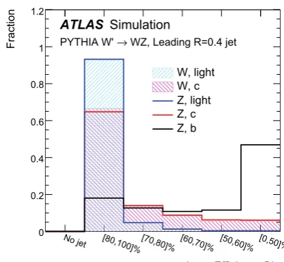
Fig. 4 The efficiency-binned MV1 distribution for small-radius jets associated with large-radius jets resulting fromWandZboson decays. Theleft(right)plotshows the leading (sub-leading) small-radius jet MV1 distribution. The bins correspond to exclusive regions ofb-jet
efficiency. As such, the bin content of theblack line(b-tagging for b-jets) should be proportional to the size of the efficiency window: about 50 % for the rightmost bin, 10 % for the three middle bins and 20 % for the second bin
ger and so all results are shown also without such variables. In a variety of physics processes, the charge of the hadroni-cally decayingW boson is known from other information in the event. For example, in searches for FCNC effects intt¯ events with one leptonically decayingW boson, the charge of the lepton is opposite to the charge of the hadronically decayingW boson. Henceforth, only W+ bosons are used for constructing the boson-type tagger; the results are the same forW−bosons.
The tracks from charged particles can be used further to identify the decays of certain heavy-flavour quarks inside jets due to the longb-hadron lifetime. This is useful for boson-type tagging because theZboson couples tobb¯while decays of theWboson tob-quarks are highly suppressed and can be neglected. ATLAS has commissioned ab-tagging algorithm called MV1 (defined in Refs. [43,44]) which combines infor-mation about track impact-parameter significance with the explicit reconstruction of displacedb- andc-hadron decay vertices. The boson-type tagger presented here uses multi-ple bins of the MV1 distribution simultaneously. Five bins of MV1 are defined byb-tag efficiencies (probability to tag ab-quark jet as such) of 0–50, 50–60, 60–70, 70–80, and 80–100 % as determined in simulatedtt¯events. A lowerb -tag efficiency leads to higher light-quark jet rejection. The fiveb-tagging efficiency bins are exclusive and MV1 is con-structed as a likelihood with values mostly between zero and one (one means more like ab-jet). For example, a 100 %b -tagging efficiency corresponds to a threshold of MV1> 0 and an 80 %b-tagging efficiency corresponds to a threshold value of MV1>zforz1. The 80–100 %b-tag efficiency bin then corresponds to jets with an MV1 value between 0
and z. Constructed in this way, the fraction of true b-jets inside an efficiency binx%–y% should be(y−x)%.
Small-radius jets are matched to a large-radius jet by geo-metric matching5(R<1.0). Of all such small-radius jets, the two leading ones are considered. There are thus 30 possi-ble bins of combined MV1 when considering the leading and sub-leading matched small-radius jet. The number of bins is 25 from the 5×5 efficiency-binned MV1 distributions in addition to five more for the case in which there is no second small-radius jet matched to the large-radius jet. The distribu-tion for the efficiency-binned MV1 variable for the leading and sub-leading matched small-radius jets is shown for W andZ bosons in Fig.4. The flavour of a small-radius jet is defined as the type of the highest energy parton from the parton shower record withinR<0.4. As expected, a clear factorization is seen in Fig.4– the MV1 value depends on the flavour of the small-radius jet and not the process that created it. This means thatc-jets fromW decays have the same MV1 distribution asc-jets fromZdecays; the same is true for light jets. Small-radius jets originating fromb-hadron decays tend to have a larger value of MV1, which means they fall in a lower efficiency bin. Small-radius jets not originating fromb -orc-decays are called light jets and are strongly peaked in the most efficient bin of MV1. There is always one small-radius jet matched to the large-radius jet, but about 20 % of the time there is no sub-leading small-radius jet with pT >25 GeV
5 In the definition of jets,Ris the characteristic size in(y, φ)and the rapidityyis used in the jet clustering procedure, whereas geometrical matching between reconstructed objects is performed using(R)2=
[image:6.595.82.290.52.243.2]Jet Mass [GeV]
0 50 100 150
Fraction / 3 GeV
0 0.05 0.1 0.15 0.2 b b → Z c c → Z light → Z cX → W light → W ATLASSimulation WZ → PYTHIA W'
= 8 TeV, s
< 400 GeV
T
200 GeV < p
(a)
=0.5) [e] κ Jet Charge (
-2 -1 0 1 2
Fraction / 0.16 e
0 0.05 0.1 0.15 0.2 0.25 b b → Z c c → Z light → Z cX → + W light → + W ATLAS Simulation WZ → PYTHIA W'
= 8 TeV, s
< 400 GeV
T
200 GeV < p
[image:7.595.118.480.54.231.2](b)
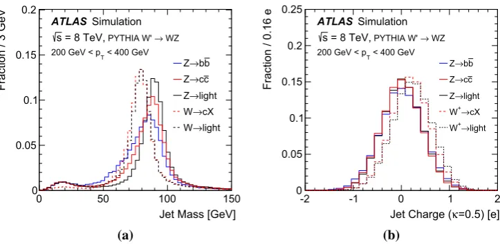
Fig. 5 aThe jet massp(M|F,V)andbjet charge p(Q|F,V)templates conditioned on the flavourFof the bosonV decay for jets with 200 GeV<pT<400 GeV. Thesolid linesare forZboson decays and thedashed linesare forWboson decays
matched to the large-radius jets. These cases are all predicted to originate from light-quark decays of theWandZbosons.
5 Tagger performance
The optimal multivariate tagger combining jet mass, jet charge, and the MV1 of matched small-radius jets is con-structed from a three-dimensional (3D) likelihood ratio. For N bins each of jet mass and jet charge, as well as 30 com-bined MV1 bins, the 3D likelihood ratio would have 30×N2 total bins. Populating all of these bins with sufficient MC events to produce templates for the likelihood ratio requires an unreasonable amount of computing resources, especially for the high-efficiency bins of combined MV1. Estimating the 3D likelihood as the product of the 1D marginal distri-butions, where all variables but the one under consideration are integrated out, is a poor approximation for jet mass and combined MV1 due to the correlation induced by the pres-ence of semileptonicb-decays, which shift the jet mass to lower values due to the presence of unmeasured neutrinos.6 It is still possible to use a simple product by noting that all three tagger inputs are independent when the flavour of the decaying boson has been determined. Thus, for each pos-sible boson decay channel, templates are built for the jet mass, the jet charge, and the efficiency-binned MV1 distri-butions. For a particular decay flavour, the joint distribution
6The muons from semileptonic decays are added back to the jet using a four-momentum sum. Muons are measured by the combination of a dedicated muon spectrometer with its own toroidal magnetic field outside the calorimeters, and the inner detector. Adding back the muon has a negligible impact on the inclusive mass distribution due to the semileptonic branching ratios and lepton identification requirements. For details about the muon reconstruction and selection, see Sect.7
(the only difference here is that the isolation is not applied).
is then the product of the individual distributions. Summing over all hadronic decay channels then gives the full distribu-tion. To ease notation, the efficiency-binned MV1 is denoted B =(Blead,Bsub-lead). The distribution forBlead(Bsub-lead) is shown in the left (right) plot in Fig.4. Symbolically, for decay flavour channelF, massM, chargeQ, and efficiency-binned MV1B, the likelihood is given by:
p(M,Q,B|V)
=
F
Pr(F|V)p(M|F,V)p(Q|F,V)Pr(B|F,V), (3)
where7V ∈ {W,Z}and the sum is overF =bb,cc,cs,cd and light-quark pairs. The distribution ofB is well approx-imated as the product of the distributions for Blead and Bsub-lead when the flavours of the leading and sub-leading jets are known. This is exploited for hadronically decay-ing W bosons and for the light-quark flavour decays of Z bosons to construct templates for B that have a suffi-cient number of simulated events for large values of B, i.e. Pr(B|F,V)=Pr(Blead|F,V)Pr(Bsub-lead|F,V). The unit-normalized templates forBare shown in Fig.4and the unit-normalized templatesp(M|F,V)andp(Q|F,V)are shown in Fig.5. For a given boson type, the jet-charge template is nearly independent of the flavour. However, there is a depen-dence of the jet mass on the (heavy) flavour of the boson decay products.
The likelihood function is constructed by taking the ratio of the probability distribution functions p(M,Q,B|V), for V ∈ {W,Z}, determined from the templates in Eq. (3). Every bini of the 3D histogram that approximatesp(M,Q,B|V) is assigned a pair of numbers(i,si/bi)wheresiis the overall
fraction of the signal (Z orW) in biniandbi is the fraction of the overall background (the other boson flavour) in bin i. Bins are then sorted from largest to smallestsi/bi, with
f(i)defining a map from the old bin index to the new, sorted one. There are then two 1D histograms: for the signal, bin j has bin contentsf−1(j)and for the background, bin jhas bin
contentbf−1(j). The optimal tagging procedure is then to set
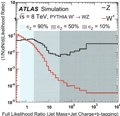
a threshold on the new 1D histograms. The full likelihood ratio of the combined tagger is shown in Fig.6 where the thresholds required for 90, 50, and 10 % Z-boson tagging efficiency are marked with shaded regions.
Full Likelihood Ratio (Jet Mass+Jet Charge+b-tagging)
1 10 102 103 104
(1/N)dN/d(Likelihood Ratio)
-5 10
-4 10
-3 10
-2 10
-1 10
1 10
= 90%
Z
∈ ∈Z = 50% ∈Z = 10%
Z
+
W ATLAS Simulation
WZ → PYTHIA W'
= 8 TeV, s
Fig. 6 The full likelihood ratio for the tagger formed from jet mass, jet charge, and a small-radius jetb-tagging discriminant. Theblack histogramshows the likelihood ratio forZbosons and thered histogram is the likelihood ratio forW+bosons. Theshaded areasshow the region of the likelihood ratio corresponding to 90, 50,and 10 % working points of theZ-boson tagging efficiency
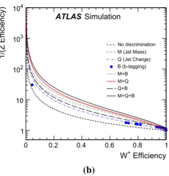
Curves displaying the tagging performance for all possi-ble subsets of{M,Q,B}are shown in Fig.7. There are 30 possible values forB, which are therefore represented by dis-crete points. The jet mass is the best performing single vari-able for medium to high Z-boson efficiencies, with visible improvement forM+BandM+Q. There is a significant gain from combining all three variables forZ-boson tagging effi-ciency above about 20 %. Below 20 %, the combined tagger is dominated byBwhere theZ →bb¯branching fraction no longer limitsZ-boson tagging efficiency. For Z-boson effi-ciencies of about 50 %, one can achieveW+rejection factors (1/W+) of 3.3 by usingQor Balone and about 5.0 using mass alone. ForZefficiencies ofZ =90, 50, and 10 %,W+ rejection factors of 1.7, 8.3, and 1000, respectively, can be achieved with the combined tagger. Although most applica-tions of boson-type tagging will targetZbosons as the signal while rejectingWbosons as background, the likelihood con-structed in Fig.6can also be used to optimally distinguish W+bosons fromZbosons. The corresponding performance curves are shown in Fig.8. The locations of the b-tagging points are all now shifted to high efficiency with respect to Fig. 7 because, for W+ tagging, one wants to operate in the high-efficiencyb-tagging bins (whereas the opposite is optimal forZ tagging). At an efficiency ofW+ = 50 %, a
Z-boson rejection factor of 1/Z ≈6.7 can be achieved.
6 Systematic uncertainties
The performance curves in Fig. 7 are based on the nomi-nal modelling parameters of the ATLAS simulation. Addi-tional studies show how the curves change due to the sys-tematic uncertainties on the inputs to the likelihood
func-Z Efficiency
Efficiency)
+
1 - (W
0 0.2 0.4 0.6 0.8 1
No discrimination M (Jet Mass) Q (Jet Charge) B (b-tagging) M+B M+Q Q+B M+Q+B
ATLASSimulation
(a)
Z Efficiency
0 0.2 0.4 0.6 0.8 1 0 0.2 0.4 0.6 0.8 1
Efficiency)
+
1/(W
1 10
2
10
3
10
4
10
No discrimination M (Jet Mass) Q (Jet Charge) B (b-tagging) M+B M+Q Q+B M+Q+B
ATLASSimulation
(b)
Fig. 7 The tradeoff betweenZefficiency anda1−(W+efficiency)b or 1/(W+efficiency) onaa linear scale andba logarithmic scale.Each curveis constructed by placing thresholds on the likelihood constructed
[image:8.595.70.268.203.394.2] [image:8.595.115.287.486.664.2]Efficiency +
W
0 0.2 0.4 0.6 0.8 1
1 - (Z Efficiency)
0 0.2 0.4 0.6 0.8 1 No discrimination M (Jet Mass) Q (Jet Charge) B (b-tagging) M+B M+Q Q+B M+Q+B ATLASSimulation (a) Efficiency + W
0 0.2 0.4 0.6 0.8 1
1/(Z Efficiency) 1 10 2 10 3 10 4 10 No discrimination M (Jet Mass) Q (Jet Charge) B (b-tagging) M+B M+Q Q+B M+Q+B ATLASSimulation (b)
Fig. 8 The tradeoff betweenW+efficiency anda1−(Zefficiency) orb1/(Zefficiency) onaa linear scale andba logarithmic scale.Each curveis constructed by placing thresholds on the likelihood constructed
from the inputs indicated in the legend. Since theb-tagging discrimi-nant is binned in efficiency, there are only discrete operating points for the tagger built only fromB
Z Efficiency
Efficiency)
+
1 - (W
0.6 0.7 0.8 0.9 1 ATLAS Simulation WZ → PYTHIA W'
= 8 TeV, s
Jet Mass Tagger 50% Benchmark
Nominal Benchmark JMS Down JMS Up JMR (20 percent) HERWIG
Z Efficiency
Efficiency)
+
1 - (W
0.1 0.2 0.3 0.4 0.5 ATLAS Simulation WZ → PYTHIA W'
= 8 TeV, s
Jet Mass Tagger 90% Benchmark
Nominal Benchmark JMS Down JMS Up JMR (20 percent) HERWIG
(a)
Z Efficiency
Efficiency)
+
1 - (W
0.6 0.65 0.7 0.75 0.8 ATLAS Simulation WZ → PYTHIA W'
= 8 TeV, s
Jet Charge Tagger 50% Benchmark
Nominal Benchmark
)
η
Track Efficiency ( JER (20 percent) HERWIG
Z Efficiency
0.3 0.4 0.5 0.6 0.7 0.7 0.8 0.9 1 1.1
0.4 0.45 0.5 0.55 0.6 0.8 0.85 0.9 0.95 1
Efficiency)
+
1 - (W
0.16 0.18 0.2 0.22
0.24 ATLAS Simulation
WZ → PYTHIA W'
= 8 TeV, s
Jet Charge Tagger 90% Benchmark
Nominal Benchmark
)
η
Track Efficiency ( JER (20 percent) HERWIG
(b)
Fig. 9 The impact of selected systematic uncertainties on benchmark working points of the boson-type tagger.aA jet-mass-only tagger, for 50 % (left) and 90 %Zefficiency benchmarks.bA jet-charge-only tag-ger, for 50 % (left) and 90 %Zefficiency benchmarks. Thepointmarked
HERWIGuses the alternative shower and hadronization model for the
[image:9.595.306.481.53.235.2] [image:9.595.114.285.55.235.2]tion. Sources of experimental uncertainty include the cali-brations of the large- and small-radius jet four-momenta, the b-tagging (which incorporates e.g. impact parameter mod-elling), and the modelling of track reconstruction.
The uncertainty on the scale of the large-radius jet mass calibration is estimated using the double ratio in data and MC simulation of calorimeter jet mass to track jet mass [45]. Tracks associated with a jet are well measured and provide an independent observable correlated with the jet energy. Uncer-tainties on the jet-mass resolution can have a non-negligible impact on the performance of the tagger. The jet-mass res-olution uncertainty is determined from the difference in the widths of the boostedWboson jet-mass peak in semileptonic tt¯simulated and measured data events [45] and also from varying the simulation according to its systematic uncertain-ties [46]. The resolution is about 5 GeV in the Gaussian core of the mass spectrum and its uncertainty is about 20 %. The impact of the jet-mass scale and resolution uncertainties on the boson-type tagger built using only the jet mass is shown in Fig.9 for two nominal working points of 50 and 90 % Z-boson tagging efficiency. Both the likelihood map f from Sect.5and the threshold value are fixed. Inputs to the tag-ger are shifted by their uncertainties and the 1D histograms described above are re-populated. The efficiencies forWand Z bosons are recomputed and shown as markers in Fig.9a. Coherent shifts of the jet masses (JMS) forW andZbosons result in movement along the nominal performance curve corresponding to±10 % changes in the efficiency. However, there are also shifts away from the nominal curve because the optimal jet-mass cut is not a simple threshold. Variation of the jet-mass resolution (JMR) preserves the scale and so the movement is nearly perpendicular to the original perfor-mance curve, at the5 % level, because of the increased overlap in the Z and W mass distributions.8 Shifts along the nominal curve optimally use the input variables (albeit at different efficiencies), while shifts away from the nomi-nal curve are a degradation in the performance. The impact of the fragmentation is estimated by using input variables fromHERWIGbut with the likelihood map fromPYTHIA. PYTHIAandHERWIGhave similarW/Zefficiencies at both the 50 and 90 % benchmark points.
The systematic uncertainty on the efficiency of the track-ing reconstruction is estimated by removtrack-ing tracks associated with jets using anη-dependent probability [47]. The prob-ability in the region 2.3 < |η| < 2.5 is 7 %; it is 4 % for 1.9 < |η| < 2.3, 3 % for 1.3 < |η| < 1.9, and 2 % for 0<|η|<1.3. These probabilities are known to be conser-vative in the most centralηbins. There is also an uncertainty on the modelling of track merging for high-pTjets, but the
8Although such shifts retain optimal use of the tagger (highest rejection for a fixed efficiency), they can degrade the quality of e.g. a cross-section measurement.
Z Efficiency
0.06 0.08 0.1 0.12 0.14
Efficiency)
+
1 / (W
3
10
ATLAS Simulation
WZ
→
PYTHIA W'
= 8 TeV, s
b-tagging Tagger 10% Benchmark
500
Nominal b-tag
Nominal b-tag Benchmark
b-jet b-tagging scale factor
c-jet b-tagging scale factor
light-jet b-tagging scale factor
[image:10.595.326.527.54.250.2]HERWIG
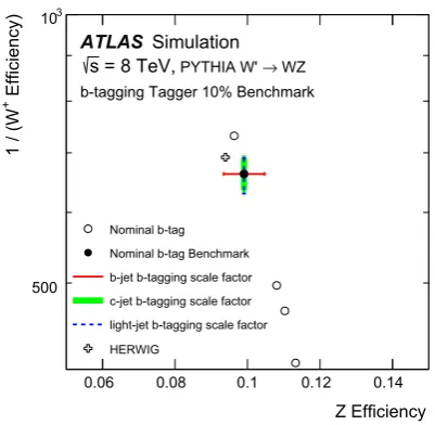
Fig. 10 The impact of selected systematic uncertainties on benchmark working points of ab-tagging-only tagger at a 10 %Zefficiency bench-mark. Theb-tagging discriminant is binned, so there are only discrete operating points. The point markedHERWIGuses the alternative shower and hadronization model for the simulation, with the likelihood template
fromPYTHIA. Theb-tagging scale factor uncertainties are determined
separately forb-,c-, and light-quark jets. Variations are added in quadra-ture for each ‘truth’ jet flavour. There is no contribution from theb-jet scale factor uncertainties on theWrejection because there are no ‘truth’ b-jets. Conversely, thec- and light-jet scale factor uncertainties do not impact theZbosons because at this low efficiency, all the selectedZ bosons decay intobb¯
Z Efficiency
Efficiency)
+
1 - (W
0.8 0.9 1
ATLAS Simulation
WZ → PYTHIA W'
= 8 TeV, s
Full Tagger 50% Benchmark
Nominal Nominal Benchmark JMS down JMS up JMR (20 percent) HERWIG
(a)
Z Efficiency
0.3 0.4 0.5 0.6 0.7 0.8 0.9 1 1.1
Efficiency)
+
1 - (W
0.2 0.3 0.4 0.5 0.6
ATLASSimulation
WZ → PYTHIA W'
= 8 TeV, s
Full Tagger 90% Benchmark
Nominal Nominal Benchmark JMS down JMS up JMR (20 percent) HERWIG
[image:11.595.312.481.54.236.2] [image:11.595.118.287.55.236.2](b)
Fig. 11 The impact of uncertainties on the jet-mass scale and reso-lution for 50 % (a) and 90 % (b) Z efficiency working points of the full boson-type tagger. ThepointmarkedHERWIGuses the alternative
shower and hadronization model for the simulation, with the likelihood template fromPYTHIA
only theb-tagging discriminant for a 10 % nominal Z effi-ciency is shown in Fig.10. At this efficiency, the full boson-type tagger is dominated by theb-tagging inputs, as seen in Fig.7. The scale factor uncertainty forb-jets has no impact on theW efficiency (no realb-jets), but there is approximately a 10 % uncertainty on theZ efficiency. The uncertainties on the jet-energy scale for small-radius jets are relevant only because of the 25 GeVpTthreshold. Since all of the large-radius jets are required to havepT>200 GeV, the threshold is relevant only in the rare case that one of theW daughters is nearly anti-parallel in theW rest frame to the direction of theW boost vector.
The impact of the uncertainties on the jet-mass scale and resolution on the boson-type tagger built using all of the inputs (jet mass, jet charge, andb-tagging) is shown in Fig.11a. At very lowZ-boson tagging efficiency, the tagger is dominated byb-tagging, so Fig.10is a good representa-tion of the uncertainty on the full tagger’s performance. For higher efficiencies, the tagger is dominated by the jet mass, although the jet charge andb-tagging discriminant signifi-cantly improve the performance. The uncertainty on the full tagger’s performance at the 50 and 90 % Z-boson tagging efficiency benchmark points is due mostly to the uncertainty on the jet mass, which is why these uncertainties are shown in Fig.11.
7 Validation of tagging variables using data
The tagger cannot be fully tested with data because it is not possible to isolate a pure sample of hadronically decaying Z bosons in pp collisions. However, the modelling of the variables used to design the tagger can be studied with a rel-atively pure and copious sample of hadronically decaying
[GeV]
T
Jet p
200 250 300 350 400
Entries / 10 GeV
0 2 4
3
10
×
2012 Data Total SM
Boosted W t t
b-Contaminated t
t Other t t Single Top W+jets multijets
ATLAS e+μ
-1
L dt = 20.3 fb
∫
= 8 TeV, s
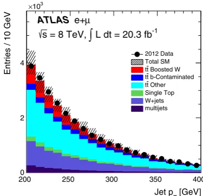
Fig. 12 ThepTdistribution of the selected large-radius jets. The uncer-tainty band includes all the experimental uncertainties on the jetpTand jet mass described in Sect.6
W bosons intt¯events which can be tagged by the leptonic decay of the other W boson in the event (semileptonic tt¯ events). Single-lepton triggers are used to reject most of the events from QCD multijet background processes. Candidate reconstructedtt¯events are chosen by requiring an electron or a muon with pT >25 GeV and|η| <2.5, as well as a missing transverse momentum ETmiss > 20GeV. The elec-trons and muons are required to satisfy a series of quality criteria, including isolation.9 Events are rejected if there is
[image:11.595.323.522.293.485.2]Entries / 5 GeV
0 0.5 1 1.5 2 2.5 3
3
10 ×
2012 Data Total SM
Boosted W t t
b-Contaminated t
t Other t t Single Top W+jets multijets
ATLAS e+μ
-1
L dt = 20.3 fb
∫
= 8 TeV, s
Jet Mass [GeV]
0 50 100 150 200
Data / MC
0.5 1 1.5
(a)
[GeV]
T
Jet p 200 250 300 350 400
Jet Mass Median [GeV]
70 80 90 100 110 120
ATLAS e+μ
-1
L dt = 20.3 fb
∫
= 8 TeV, s
< 120 GeV
jet
50 GeV < m
2012 Data
Total SM
(b)
[GeV]
T
Jet p 200 250 300 350 400
Jet Mass Inter-quantile Range [GeV] 0
10 20 30
ATLAS e+μ
-1
L dt = 20.3 fb
∫
= 8 TeV, s
< 120 GeV
jet
50 GeV < m
2012 Data 20% Total SM 20%
2012 Data 30% Total SM 30%
2012 Data 40% Total SM 40%
[image:12.595.112.485.52.509.2](c)
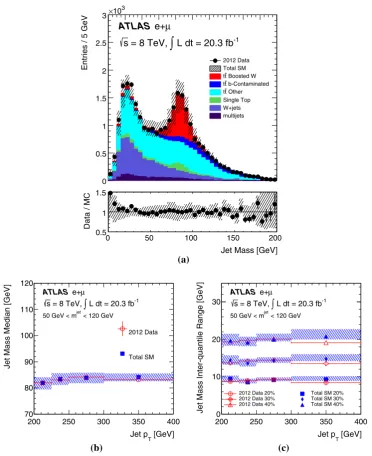
Fig. 13 aThe jet-mass distribution of the selected jets in semi-leptonic tt¯events.bThe median of the mass distribution as a function of the jetpTfor events with the selected jet in the range 50 GeV<mjet< 120 GeV. This includes the contributions from events which are not clas-sified as BoostedW.cFor the same events as inb, the inter-quantile range as a measure of spread. The quantiles are centred at the median.
The uncertainty band includes all the experimental uncertainties on the jetpTand jet mass described in Sect.6. The inter-quantile range of size 0 %<X<50 % is defined as the difference between the 50 %+X% quantile and the 50 %−X% quantile. Statistical uncertainty bars are included on the data points but are smaller than the markers in many bins
not exactly one electron or muon. In addition, the sum of theEmissT and the transverse mass10of theW boson, recon-structed from the lepton andETmiss, is required to be greater than 60 GeV. Events must have at least oneb-tagged jet (at the 70 % efficiency working point) and have at least one large-radius trimmed jet withpT>200 GeV and|η|<2.
Further-10The transverse mass,m
T, is defined as m2T = 2p lep
T ETmiss(1−
cos(φ)), whereφis the azimuthal angle between the lepton and the direction of the missing transverse momentum.
more, there must be a small-radius jet withpT>25 GeV, and
Entries / 0.05
0 1 2
3
10
×
2012 Data Total SM
Boosted W t t
b-Contaminated t
t Other t t Single Top W+jets multijets
ATLAS e+μ
-1
L dt = 20.3 fb
∫
= 8 TeV, s
< 120 GeV
jet
50 GeV < m
= Jet mass (tracks) / Jet mass (calo)
track
r
0 0.5 1 1.5
Data / MC
0.5 1 1.5
(a)
[GeV]
T
Jet p 200 250 300 350 400
Median
track
r
0.4 0.5 0.6 0.7
ATLAS e+μ
-1
L dt = 20.3 fb
∫
= 8 TeV, s
< 120 GeV
jet
50 GeV < m
2012 Data
Total SM
(b)
[GeV]
T
Jet p 200 250 300 350 400
Inter-quantile Range
track
r
0 0.1 0.2 0.3
ATLAS e+μ
-1
L dt = 20.3 fb
∫
= 8 TeV, s
< 120 GeV
jet
50 GeV < m
2012 Data 20% Total SM 20% 2012 Data 30% Total SM 30% 2012 Data 40% Total SM 40%
[image:13.595.109.483.53.500.2](c)
Fig. 14 aThe distribution ofrtrack in the data for semi-leptonictt¯ events with the selected jet in the range 50 GeV<mjet<120 GeV. bThe median of thertrackdistribution as a function of the jetpT. This includes the contributions from events that are not classified as Boosted W.cThe inter-quantile range as a measure of the width. The quantiles are centred at the median. The uncertainty band includes all the
exper-imental uncertainties on the jet pTand jet mass described in Sect.6. The inter-quantile range of size 0 % < X < 50 % is defined as the difference between the 50 %+X% quantile and the 50 %−X% quan-tile. Statistical uncertainty bars are included on the data points but are smaller than the markers in many bins
to have a hightt¯purity (about 75 %), the events cannot be compared directly to the isolatedW bosons from the sim-ulatedW boson decays. This is because there are several effects that make the typical large-radius jet in semileptonic tt¯events different from isolatedW andZ boson jets inW boson events:11
11When controlling for all differences, the distributions for isolatedW bosons fromtt¯and fromWare nearly identical.
1. The event selection is based on the reconstructed jet pT (earlier sections usedpTV), so even ifpjetT 200 GeV for anR=1.0 jet, the true hadronically decayingW boson in the event may have pTW < 200 GeV and thus the W boson decay products might not be collimated within
R<1.
Entries / 2
0 1 2
3
10 ×
2012 Data Total SM
Boosted W t t
b-Contaminated t
t Other t t Single Top W+jets multijets
ATLAS e+μ
-1
L dt = 20.3 fb
∫
= 8 TeV, s
< 120 GeV
jet
50 GeV < m
tracks
n
0 10 20 30 40
Data / MC
0.5 1 1.5
(a)
[GeV]
T
Jet p 200 250 300 350 400
Median
track
n
18 20 22 24
26 ATLAS e+μ -1
L dt = 20.3 fb
∫
= 8 TeV, s
< 120 GeV
jet
50 GeV < m
2012 Data
Total SM
(b)
[GeV]
T
Jet p 200 250 300 350 400
Inter-quantile Range
track
n
0 5 10
ATLAS e+μ
-1
L dt = 20.3 fb
∫
= 8 TeV, s
< 120 GeV
jet
50 GeV < m
2012 Data 20% Total SM 20% 2012 Data 30% Total SM 30% 2012 Data 40% Total SM 40%
[image:14.595.114.484.51.508.2](c)
Fig. 15 aThe distribution of the number of tracks associated with the selected large-radius jet in the semi-leptonictt¯data for events with the selected jet in the range 50 GeV< mjet <120 GeV.bThe median of the distribution of the number of tracks as a function of the jetpT. This includes the contributions from events that are not classified as BoostedW.cThe inter-quantile range as a measure of the width. The
quantiles are centred at the median. The uncertainty band includes all the experimental uncertainties on the jetpTand jet mass described in Sect.6. The inter-quantile range of size 0 %<X<50 % is defined as the difference between the 50 %+X% quantile and the 50 %−X% quantile. Statistical uncertainty bars are included on the data points but are smaller than the markers in many bins
from the same top-quark as the hadronically decayingW bosons can merge with theW boson decay products to form a large-radius jet.
The variables pTjet/pTW and R(jet,W), for the W boson from the MC ‘truth’ record and the selected large-radius jet, are used to classify the varioustt¯event sub-topologies. Events are labelled as having aBoostedWif|pjet/pW−1|<
0.1 andR(jet,W) <0.1. If theb-quark from the top-quark decay has an angular distanceR <1.0 from the selected large-radius jet, this jet is labelled asb-contaminated. All othertt¯events, including events where bothWbosons decay into leptons, are labelled asOther. The pTspectrum of the jets from the classified events is shown in Fig.12. In Fig.12
Entries / 0.16 e
0 0.2 0.4 0.6 0.8 1 1.2 1.4 1.6 1.8
3
10 ×
Lepton Charge < 0
2012 Data
Boosted W t t
Other Lepton Charge > 0
2012 Data
Boosted W t t
Other
ATLAS e+μ
-1
L dt = 20.3 fb
∫
= 8 TeV, s
< 120 GeV
jet
50 GeV < m
=0.5) [e] κ Jet Charge (
-2 -1 0 1 2
Data / MC
0.5 1 1.5
(a)
[GeV]
T
Jet p 200 250 300 350 400
Jet Charge Median [e]
-0.5 0
0.5 ATLASe+μ
-1
L dt = 20.3 fb
∫
= 8 TeV, s
< 120 GeV
jet
50 GeV < m
Lepton Charge > 0
2012 Data Total SM
Boosted W t t Lepton Charge < 0
2012 Data Total SM
Boosted W t t
(b)
[GeV]
T
Jet p 200 250 300 350 400
Jet Charge Inter-quartile Range [e]
0.4 0.5 0.6 0.7 0.8
ATLASe+μ
-1
L dt = 20.3 fb
∫
= 8 TeV, s
< 120 GeV
jet
50 GeV < m
2012 Data Total SM
Boosted W t
t
[image:15.595.115.487.56.518.2](c)
Fig. 16 aThe distribution of the jet charge in the data for semi-leptonic tt¯events with the selected jet in the range 50 GeV<mjet<120 GeV. The ratio uses the positive lepton charge.bThe median of the jet charge distribution as a function of the jetpT. This includes the contributions from events that are not classified as BoostedW(except for theblue tri-angles, for which only the BoostedWis included).cThe inter-quartile
range as a measure of the width. The quantiles are centred at the median. The uncertainty band includes all the experimental uncertainties on the jet pT and jet mass described in Sect.6. The inter-quantile range is defined as the difference between the 75 % quantile and the 25 % quan-tile. Statistical uncertainty bars are included on the data points but are smaller than the markers in many bins
in Sect.6, but exclude tracking uncertainties, which are sub-dominant. Events are vetoed if the selected large-radius jet haspT>400 GeV or if theRbetween the selected large-radius jet and a taggedb-jet is less than 1.0. This suppresses theb-contaminatedtt¯events. The effectiveness of thett¯event classification is most easily seen from the jet mass distribu-tion, shown in Fig.13a. The mass of the boostedW bosons fromtt¯events is peaked aroundmW, as is a small
Entries
0 5 10 15 20
3
10
×
2012 Data Total SM
Boosted W t t
b-Contaminated t
t Other t t Single Top W+jets multijets
ATLAS e+μ
-1
L dt = 20.3 fb
∫
= 8 TeV, s
b-tag Efficiency Bin No je
t [80,100]% [70,80]% [60,70]% [50,60]% [0,50]%
Data / MC
0.5 1 1.5
(a)
Entries
0 10 20
3
10
×
2012 Data Total SM
Boosted W t t
b-Contaminated t
t Other t t Single Top W+jets multijets
ATLAS e+μ
-1
L dt = 20.3 fb
∫
= 8 TeV, s
b-tag Efficiency Bin No jet [80,100]% [70,80]% [60,7
0]% [50,60]% [0,50]%
Data / MC
0.5 1 1.5
[image:16.595.308.506.53.325.2](b)
Fig. 17 The efficiency-binned MV1 distribution for thealeading and bsub-leading matched small-radius in semi-leptonictt¯events. If there is no second small-radius jet withpT >25 GeV andR<1 to the selected large-radius jet axis, the event is put in the ‘No jet’ category in
b. The uncertainty band includes all the experimental uncertainties on the jetpTand jet mass and those related to theb-tagging described in Sect.6. Statistical uncertainty bars are included on the data points but are smaller than the markers in many bins
inW+jets and the ‘other’tt¯events is due to the Sudakov peak from QCD jets, the location of which scales withR× pT. The dependence on pTof the W-peak position in Fig.13a is shown in Fig.13b. Events with the leading jet in a win-dow around theW mass, 50 GeV< mjet < 120 GeV are selected and the median of the mass distribution is plotted in Fig.13b as a function of the jetpT. The similar trend for the simulation and the data shows that the combination of the reconstructed jet-mass scale and ‘truth’ jet-mass scale is well modelled. To quantify the spread in the jet mass peak, various inter-quantile ranges are shown as a function ofpTin Fig.13c. The inter-quantile range of size 0 %< X <50 % is defined as the difference between the 50 %+X% quantile and the 50 %−X% quantile, and is a measure of the spread in the distribution. The width of the boosted-W mass peak is well modelled within the statistical precision of the 2012 data sample.
The modelling of boosted W bosons can also be stud-ied using the jet-mass scale measured from tracks. Defining the variablertrackas the ratio of the jet mass determined from tracks to the jet mass determined from the calorimeter, the jet mass scale uncertainty is related to the difference from unity of the ratio ofrtrack in data tortrack in MC simulation. The mass scale uncertainty is calculated using the procedure described above, but withrtrack−1 . If the jet consists only of
[image:16.595.84.285.58.323.2][GeV] T Boson p
200 400 600 800 1000
[GeV]
〉
Jet Mass
〈
0 20 40 60 80 100 120 140 160 180
ATLAS Simulation = 8 TeV s
WZ → PYTHIA W'
Z
W
(a)
[GeV] T Boson p
200 400 600 800 1000
[e]
〉
=0.5)
κ
Jet Charge (
〈
-0.2 -0.1 0 0.1 0.2 0.3 0.4 0.5 0.6 0.7 0.8
ATLASSimulation = 8 TeV s
WZ → PYTHIA W'
Z
+ W
(b)
[GeV] T Boson p
200 400 600 800 1000
〉
Matched b-jet Multiplicity
〈
0 0.2 0.4 0.6 0.8 1 1.2 1.4
ATLASSimulation = 8 TeV s
WZ → PYTHIA W'
Z
W
[image:17.595.111.481.53.393.2](c)
Fig. 18 The bosonpTdependence of theajet mass,bjet charge, andcnumber of small-radiusb-tagged jets matched to the large-radius jet
acceptance for charged particles from the boostedW boson decay. The width is well modelled within the statistical pre-cision of the data. However, there is disagreement for the median. Previous studies (including Rev. [50]) suggest that this is due to fragmentation modelling and not the modelling of the detector response.
ThepT-weighted distribution of the track charges defines the jet charge, which is shown in Fig.16a. The charge of the lepton from the leptonicW boson decay determines the expected charge of the hadronically decayingW boson can-didate, allowing for a tag-and-probe study of the capability of charge tagging in hadronicW boson decays [42]. The jet charge for boostedW bosons for positively (negatively) charged leptons is clearly shifted to the left (right) of zero. There is also some separation between positive and nega-tiveW boson decays when the selected large-radius jet does not satisfy the criteria for being a boosted W boson. This is because the jet still contains some of theW boson decay products, and the jet charge is correlated with the charge of theW boson. The difference between the inclusive and boostedW-boson jets is clearer in thepTdependence plot of
the median jet charge shown in Fig.16b. The medians of the distributions for boostedW jets are nearly twice as far apart as the medians for inclusive jets. However, in both cases the spread is less than the width of the distribution, shown as the inter-quantile range (inter-quantile range withX =25 %) in Fig.16c. Even though there is some small disagreement for the median number of tracks, thepT-weighted sum defining the jet charge is reasonably well modelled.
The remaining input to the boson tagger is the b -tagging discriminant for the matched small-radius jets. The efficiency-binned MV1 distributions are shown in Fig.17a, b with the same selection criteria as for the previous figures, except that theb-jet veto is removed. The contamination due to the b-jet from the top-quark decay complicates a direct study of the MV1 distribution for boostedW jets; contami-nation from theb-quark decay products is seen clearly in the MV1 distribution at lower values of the efficiency. Most of the boostedW jets are in the highest efficiency bin because they have no realb-hadron decay.
8 Outlook
The simulation studies of the boson-type tagger presented in Sect.5show that for bosons with 200 GeV< pT<400 GeV, it is possible to achieveZ-boson efficiencies ofZ =90, 50, and 10 % withW+ boson rejections of 1.7,8.3 and 1000, respectively. Putting this into context, with R(Z)defined as the lowest possibleW-boson tagging efficiency at a fixed Z-boson tagging efficiency:
• TheW Z/W W cross-section ratio is∼20 % [51]. At the 50 % type-tagger working point, one can change the ratio of events to
50 % R(50 %)×
σ (W Z) σ(W W)=
50 % 12 %×
σ (W Z) σ (W W)
= 50
12×20 %≈83 %, (4) with the possibility for a high-purity extraction of the W Zcross section in the semileptonic channel (νqq¯).
• Diboson resonances are predicted by many models of physics beyond the Standard Model. The all-hadronic channel provides a significantly higher yield than the lep-tonic channels. At the 90 % type-tagger working point, one can distinguishZ ZfromW Zwith a likelihood ratio of 0.92/(0.9×0.6)∼1.5. new resonance is discovered with∼20 events, this means that the difference between Z Z andW Z is distinguishable within a 2σ statistical uncertainty of the data.
• At the 10 % type-tagger working point, a leptophobic flavour-changing neutral current intt¯production (with decays like in the SM) with a branching ratio of 1 % would have the same number of events as thet →bW decay:12
10 % R(10 %)×
(t →Z c) (t→W b) =
10 % 0.1 % ×
(t→ Z c) (t →W b)
=100×1 %=100 %. (5)
Only the range 200 GeV< pT <400 GeV was studied thus far due to the availability ofW bosons in the data. Fig-ure18shows how the average and standard deviation of the jet mass, jet charge and multiplicity of the matched small-radius b-tagged jets distributions depend on jetpTin simulation up to 1 TeV. As long as the jetpTis high enough so that a single jet captures all of the boson decay products, the jet mass and jet charge distributions are predicted to be largely indepen-dent ofpT. The information fromb-tagging degrades around 400 GeV as the two decay products from the boson become too close to resolve two separate jets.
12Up to impurities due to the high-occupancytt¯environment.
9 Conclusions
A tagger for distinguishing hadronically decaying boostedZ bosons fromW bosons using the ATLAS detector has been presented. It will most likely be used after a boson tagger has rejected most QCD multijet events. Three discriminat-ing variables are chosen which are sensitive to the differences in boson mass, charge, and branching ratios to specific quark flavours: large-radius jet mass, large-radius jet charge, and an associated small-radius jetb-tagging discriminant. For mod-erate and high Z-boson tagging efficiencies, the jet mass is the most discriminating of the three variables, but there is significant improvement in discrimination when combining all three inputs into a single tagger. At lowZ-boson efficien-cies, smaller than theZ →bb¯branching ratio, theb-tagging discriminant is the most useful for rejectingW bosons. The full tagger is largely unaffected by many systematic uncer-tainties on the inputs, with the exception of the unceruncer-tainties on the jet-mass scale and resolution. While it is not possible to measure the tagger efficiencies directly in data due to the lack of a pure sample of boosted, hadronically decaying Z bosons, modelling of the likelihood function using hadroni-cally decayingW bosons has been studied in the data. Over-all, the simulation agrees well with the 20.3 fb−1of√s=8 TeVppdata collected at the LHC.
PIC (Spain), ASGC (Taiwan), RAL (UK) and BNL (USA) and in the Tier-2 facilities worldwide.
Open Access This article is distributed under the terms of the Creative Commons Attribution 4.0 International License (http://creativecomm ons.org/licenses/by/4.0/), which permits unrestricted use, distribution, and reproduction in any medium, provided you give appropriate credit to the original author(s) and the source, provide a link to the Creative Commons license, and indicate if changes were made.
Funded by SCOAP3.
A. Correlations with 2-subjettiness
The tagger developed in this paper is designed to work in conjunction with a procedure for separating generic quark and gluon jets from boson jets. Figure19 shows the joint distribution of the jet mass and jet charge with a standard boson tagging variable 2-subjettiness,τ21. The boson type tagger variables are nearly independent ofτ21.
Arbitrary Units
-2
10
-1
10 1
21 τ 2-subjettiness
Jet Mass [GeV]
60 80 100 120
ATLAS Simulation
< 400 GeV
T
Hadronic W, 200 GeV < p
Correlation: 0.05
Arbitrary Units
-2
10
-1
10 1
21 τ 2-subjettiness
Jet Mass [GeV]
60 80 100 120
ATLAS Simulation
< 400 GeV
T
Hadronic Z, 200 GeV < p
Correlation: -0.08
(a)
Arbitrary Units
-2
10
-1
10 1
21 τ 2-subjettiness
=0.5) [e]
κ
Jet Charge (
-2 -1 0 1 2
ATLAS Simulation
< 400 GeV
T
Hadronic W, 200 GeV < p
Correlation: -0.02
Arbitrary Units
-2
10
-1
10 1
21 τ 2-subjettiness
0 0.2 0.4 0.6 0.8 1 0 0.2 0.4 0.6 0.8 1
0 0.2 0.4 0.6 0.8 1 0 0.2 0.4 0.6 0.8 1
=0.5) [e]
κ
Jet Charge (
-2 -1 0 1 2
ATLAS Simulation
< 400 GeV
T
Hadronic Z, 200 GeV < p
Correlation: -0.00
[image:19.595.116.481.193.576.2](b)