Adaptive Haar wavelets for the angular discretisation of spectral wave models

spectral wave models

.

White Rose Research Online URL for this paper:

http://eprints.whiterose.ac.uk/98124/

Version: Published Version

Article:

Adam, Alexandros, Buchan, Andrew G., Piggott, Matthew D. et al. (3 more authors) (2016)

Adaptive Haar wavelets for the angular discretisation of spectral wave models. Journal of

Computational Physics. pp. 521-538. ISSN 0021-9991

https://doi.org/10.1016/j.jcp.2015.10.046

[email protected]

https://eprints.whiterose.ac.uk/

Reuse

This article is distributed under the terms of the Creative Commons Attribution (CC BY) licence. This licence

allows you to distribute, remix, tweak, and build upon the work, even commercially, as long as you credit the

authors for the original work. More information and the full terms of the licence here:

https://creativecommons.org/licenses/

Takedown

If you consider content in White Rose Research Online to be in breach of UK law, please notify us by

Contents lists available atScienceDirect

Journal

of

Computational

Physics

www.elsevier.com/locate/jcp

Adaptive

Haar

wavelets

for

the

angular

discretisation

of

spectral

wave

models

Alexandros Adam

a

,

∗

_,

_Andrew

_{G. Buchan}

a

_,

_Matthew

_{D. Piggott}

a

_,

Christopher C. Pain

a

,

Jon Hill

b

,

Mark

A. Goffin

a

a_{AppliedModellingandComputationGroup,DepartmentofEarthScienceandEngineering,ImperialCollegeLondon,SW72AZ,UK} b_{EnvironmentDepartment,UniversityofYork,Heslington,YorkYO105DD,UK}

a

r

t

i

c

l

e

i

n

f

o

a

b

s

t

r

a

c

t

Articlehistory: Received29May2015

Receivedinrevisedform25October2015 Accepted26October2015

Availableonline2November2015

Keywords:

Spectralwavemodelling Actionbalanceequation Adaptivity

Angularadaptivity Haarwavelets

Anewframeworkforapplyinganisotropicangularadaptivityinspectralwavemodellingis presented.Theangulardimensionoftheactionbalanceequationisdiscretisedwiththeuse ofHaar wavelets,hierarchical piecewise-constantbasis functions withcompact support, and an adaptivemethodologyfor anisotropicallyadjusting theresolution ofthe angular meshisproposed.Thisworkallowsareductionofcomputationaleffortinspectralwave modelling,throughareductioninthedegrees offreedomrequiredforagivenaccuracy, withanautomatedprocedureandminimalcost.

2015TheAuthors.PublishedbyElsevierInc.ThisisanopenaccessarticleundertheCC BYlicense(http://creativecommons.org/licenses/by/4.0/).

1. Introduction

Awiderangeofdifferentnumericalmodelsarenowavailablewhichcanbeusedforthestudyofwavegenerationand propagation.Thesecanbesplitintotwomaincategories:phase-resolvingandphase-averaging[1].Phase-resolvingmodels, suchaspotentialflow,mild-slope,Boussinesqandfull3DNavier–Stokesmodelsrepresenttheseasurfaceelevationinspace and time andaccurately account forthe non-linear processes. They are, however, computationally expensive and, thus, restrictedto relatively smallscale applications.Phase-averaging models are basedon a spectral descriptionof thewaves andthoughthenon-linearitiesarerepresentedbyparametrised formulations,theyarecheap enoughtobeusedonlarger problemdomains.

Spectral wave modelling first appeared after the introduction of the wave energy spectrum by Pierson [2] and the introductionoftheenergybalanceequationbyGelci[3].Basedonlinearwavetheory,theseasurfaceelevationiscomposed ofasuperpositionofharmonicwavecomponentsandtheenergyspectrumE

(

x

,

y

,

f

,

θ,

t

)

representstheenergycontentover frequencies f anddirections

θ

,inspace

(

x

,

y

)

andtimet.Alloftheimportantcharacteristicsoftheseasurface,suchasthe significant waveheight orthemeanperiod,can thenbe seenasstatisticalparametersofthe spectrumandderived from variouscombinationsofitsmomentsmn

=

fnE

(

f

,

θ )

df d

θ

[4].

The energy spectrum is calculated based on the conservation of energy in an Eulerian framework. A kinematic part representing the propagation of wave energy is balanced with a set of source terms which represent wind generation, non-linearenergytransfersandwave dissipation.Variousspectralwave modelshavebeendevelopedfromasearly asthe

*

Correspondingauthor.

E-mailaddress:[email protected](A. Adam).

http://dx.doi.org/10.1016/j.jcp.2015.10.046

1960s.So-called“first-generation models”didnot account(or looselyaccounted) fornon-linearwaveenergyinteractions. “Second-generation”models useda simplifiedparametrised formfortheseinteractions, restrictingtheshape ofthe spec-trum.A thoroughreviewoftheseearlymodelscanbefoundin[5].

The next milestone in spectral wave modelling came from the WAMDI group [6] with the introduction of WAM, a model with improved formulations for the source terms andno a-priori restriction on the shape of the spectrum. This framework wascoinedas“third-generation”wavemodellingandfollowedbyrapiddevelopments.Currentswere included in the formulationby rewriting the governing equation in terms of the action density A

=

E

/

f, which is conserved in a relative frameofreferencemoving withthecurrent[7].The actionbalance equationwas then extendedto accountfor shallowwaterpropagation,suchasshoalingandrefractionandshallowwaternon-linearprocesses,suchastriadsanddepth induced breaking.Forathoroughreviewofthemostnotabledevelopmentsthereadercanreferto[8]and[9].Today the mostwidelyused thirdgenerationmodelsby thecommunityare WAM[6]andWAVEWATCHIII[10]forglobalscalesand SWAN[11]forcoastalapplications.

The sourceparameterisations and thenumericalschemesforspectral wavemodels arestill anactive fieldofresearch. Thelastfiveyears,forexample,hasseentheerrorlevelsforthepredictionofsignificantwaveheightsandmeanperiodsin themiddleoftheoceandropby20% and30% respectively[12].Afurtherreductionintheseerrorsnecessitatesanincrease incomputationalresolution,toresolvecoastalprocesseswhilestillcoveringlargedomains[13].Animportantsteptowards thisdirectionhasbeentheuseofunstructuredmeshesforthespatialdiscretisation[14–17].

Inthe oceancirculationmodellingcommunity,the widerangeofspatialandtemporalscaleshasmotivatedthe devel-opmentofspatiallyadaptiveschemes,asameansoflocalandanisotropicdynamicalmeshrefinement.Varioustechniques havebeendeveloped,withexamplesincludingthestructured tree-basedhierarchicalfinitevolume Gerris[18] modeland theunstructuredfiniteelementFluidity[19] model.The firstefforttoapplythesetechniquestotheenergybalance equa-tionwasmadebyPopinetetal.[20]whocombinedtheadaptivesolverofGerriswithWAVEWATCHIIItodevelopaspatially adaptive spectralwave model.Intheir work theyshoweda decreaseofone totwoorders ofmagnitudeinrun-timesfor practical spatial resolutions.MorerecentlyMeixner[21] was thefirsttoapply adaptivity inphasespace. Bydevelopinga discontinuousfiniteelementspectralwavemodel,p-adaptivitywasappliedbothingeographicandspectralspace.Adjusting theorderofthefiniteelementexpansionsgavesignificantspeed-upscomparedtousinguniformhigherorderexpansions, inadeepwaterpropagationtestcase.

Thisworkfocusesonapplyingadaptivity fortherefinementoftheangularresolution.Itisnoteasytoquantifythe di-rectionaldistributionofoceanwavesinageneralframework.Observations,however,showthatthedirectionaldistribution tends to be sharp around the peak frequency [22,23]. As waves propagate outside of their generation area, direction-dispersion further enhances this. Thus, in many cases the energy spectrum only contains energy in a narrow band of directions.(Thisisevenmoreobviousincoastalareaswherewavesappeartocomefromasingledirection.) Viewedinthis perspective,uniformangularresolutionsinspectralwavemodelsareinefficientsinceforaspecificpointnotallangleshave non-zero energy. Theadaptive approach proposed hereattemptsto deal withthisproblemthough the useof compactly supportedwaveletbasisfunctions.Thesecanlocallyresolvedetailsintheangulardimensionresultinginadifferentangular meshforeachcomputationalpoint.

Wavelets, became an active field of research in the 1980s, withthe worksof researchers such as Morlet, Grossman and Daubechies [24] on signal processing. Starting asan alternative toFourier analysis, their popularitysoon expanded, owing mainly tothe localised natureof waveletbasis infrequencyandtime, aswell astheir hierarchicalstructure. This meant that alocalised wavelettransformcould be performedwitha variable-resolutionreconstructionofa signal,which is ideal forapplications such as dataand image compression [25–27]. Theseadvantages soon drew the attentionof the numericalmodellingcommunity,astheaforementionedpropertiesprovidedanefficientframeworkforadaptivealgorithms. Since then, wavelets havebeen applied to various fieldsof numerical analysis, including turbulence modelling [28] and partial differential equationssuch astheNavier–Stokes[29,30],hyperbolic [31,32]andparabolic systems[33,34].A more comprehensivelistofwaveletsusedinPDE’scanbefoundin[35].

Ofmorerelevancetothiswork,istheuseofwaveletsforthediscretisationoftheBoltzmanntransportequation,which provides a natural framework forspectral wave modelling. Both the Boltzmann transport (in non-scatteringmedia) and the energy balance equations are multi-dimensionalhyperbolic systems,dealing withthe propagation ofan energyflux in geographic andphase space [36]. It is worth noting that the energybalance equation is alsoknown as theradiative transfer equation. Inthe casewhereonly four-wave interactions are considered forthesource termsit isalso knownas theBoltzmannequation[37,p. 30].Buchanetal.[38]firstappliedlinearandquadraticwaveletsforresolvingtheangular dependence of the Boltzmanntransport equation, and then went onto show how they can be used forthe application ofangularadaptivity [39].Goffinetal.[40] thenextendedthisto applygoal-basedmeasures totheerrormetrics driving adaptivity.

A. Adam et al. / Journal of Computational Physics 305 (2016) 521–538

Thepaperisorganisedasfollows.FirstinSection2theactionbalanceequationanditsdiscretisationispresented.Then inSection3abrieftheoreticalbackgroundofwaveletsisgivenandtheHaarwaveletfunctionsareintroduced.Thisisthen followedbythedevelopmentoftheadaptiveframeworkandthedescriptionoftheadaptivealgorithminSection4.Finally inSection5angularadaptivityisappliedonbothstationaryandtime-dependenttestcasesandthebenefitsofthescheme arequantified,intermsoftherequireddegreesoffreedomaswellascomputationalrun-times.Thepaperconcludeswith ageneraloverviewoftheresults.

2. Actionbalanceequation

2.1. Introduction

TheactionbalanceequationinCartesiancoordinatescanbewrittenas[4]

∂

N

∂

t

+

∂(c

gx

+

ux

)N

∂

x

+

∂(c

gy

+

uy

)N

∂

y

+

∂c

σN

∂

σ

+

∂

cθN

∂θ

=

Stot

σ

,

(1)

where the action density spectrum N

(

r

,

θ,

σ

,

t

)

(

Jm−2_rad−3_s2

₎

_{is dependent on geographical space r}

₌

₍

_x

_,

_y

₎

₍

_m

₎

_,

spec-tral space

(θ,

σ

)

, i.e. direction of travel

θ (

rad

)

and relative frequency

σ

=

2

π

f

(

rad s−1

₎

_{, the frequency in a frame}

of reference moving with the current, and time t

(

s

)

. Here Stot

(

Jm−2rad−2s

)

are the source terms, cg

=

(

cgx

,

cgy

)

=

cgcos

(θ ),

cgsin

(θ )

(

ms−1

)

isthe groupvelocity, u

=

(

ux

,

uy

)

(

ms−1

)

isthecurrentvelocityandcσ

(

rad s−2

)

,cθ

(

rad s−1

)

,

arethepropagationspeedsinthefrequencyandangledimensionrespectively.Thesepropagationspeedsare

cg

=

1 2

(

1

+

2kd

sinh

(

2kd)

)

gtanh

(kd)

k

,

(2)

cσ

=

d

σ

dt

=

∂

σ

∂

d

∂d

∂t

+

u

· ∇

d

−

cgk

·

∂

u

∂

s

,

(3)

cθ

=

dθ dt

= −

1

k

∂

σ

∂

d

∂d

∂m

+

k

·

∂

u

∂m

,

(4)

wherek

=

2

π

/

L

(

rad m−1

)

isthewavenumberandk

=

kcos

(θ ),

ksin

(θ )

thewavenumbervector, L

(

m

)

isthewavelength, d

(

m

)

thebathymetricvalue,g

(

ms−2

₎

_{theaccelerationduetogravity,ands}

₍

_m

₎

_{isacoordinateinthedirectionof}

propaga-tion

ˆ

s

=

cos

(θ ),

sin

(θ )

,whilem

(

m

)

isacoordinateperpendiculartothedirectionofpropagationm

ˆ

=

−

sin

(θ ),

cos

(θ )

.To evaluatetheseexpressionsthevalueofthewavenumberisneeded,whichcanbecalculatedfromthedispersionrelationship inarelativeframeofreference,i.e.aframeofreferencemovingwiththecurrent,

σ

2

=

gktanh

(kd).

(5)

2.2. Angulardiscretisation

Inthiswork,forsimplicity,wave-currentinteractionsandsourcetermsareneglected.Omittingthese,theactionbalance equationbecomes

∂

N(r

,t, θ )

∂

t

+ ∇ ·

cg

(

r

,

t, θ )N(r

,t, θ )

+

∂

cθ

(

r

,t, θ )N(

r

,t

, θ )

∂θ

=

0

.

(6)

Afiniteelementexpansionisusedfortherepresentationoftheangulardimension.Anarbitraryangulardiscretisationis considered,inwhich

θ

isrepresentedbythespanofangulartrialfunctionsGj, j

∈ {

1

,

2

,

. . . ,

K

}

,suchthat

N(r

,

t, θ )

≈

K

j=1

Nj

(

r

,t)G

j

(θ ).

(7)

Toderive theweakformulationoftheproblemasetoftestfunctionsisrequired.ForthisworktheGalerkinmethodis used[43],inwhich thetrialandtest functionsare thesame.Weighting theaction balanceequation withtheset oftest functionsGi,i

∈ {

1

,

2

,

. . . ,

K

}

,gives

θ

Gi

(θ )

∂

N(r

,

t, θ )

∂t

dθ

+

θ

Gi

(θ )

∇ ·

cg

(

r

,t

, θ )N(

r

,

t, θ ) dθ

+

θ

Gi

(θ )

∂

cθ

(

r

,t, θ )N(

r

,t

, θ )

∂θ

dθ

=

0

,

∀

i

∈ {

1

,

2

, . . . ,

K

}

,

[image:5.561.46.497.286.621.2]

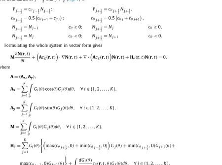
Fig. 1.Example of an element jof the angular dimensionθ, the angular fluxFj±1/2and the normalsnˆθat the element boundaries.

where

θ

istheone-dimensionalangularcoordinate.Forthelasttermof(8),applyingthedivergencetheoremgives

θ

Gi

(θ )

∂c

θ

(

r

,t, θ )N(

r

,

t, θ )

∂θ

dθ

=

S

Gi

(θ )c

θ

(

r

,t

, θ )N(

r

,t, θ )

n

ˆ

θdS

−

θ

dGi

(θ )

dθ cθ

(

r

,t, θ )N(

r

,

t, θ )dθ,

∀

i

∈ {

1

,

2

, . . . ,

K

}

,

(9)

where S corresponds to the boundary surface and n

ˆ

θ to the outward normal unit vector. Given that the domain

θ

is

one-dimensionalSreducestoapointandn

ˆ

θ is1and

−

1 onthetwoboundarynodesofeachangularelementrespectively

(Fig. 1).

Afirst-orderupwindschemeisappliedtoresolvetheangularinter-elementboundaryconditions.Thisisusedtoensure thesuccessfulimplementationofthenumericalschemes,duetoits simplicityandnumericalstability,beforehigherorder approximationsareapplied(suchastheQUICKESTscheme[44]).Foraspecificangularelement j theflux F

=

cθN fromthe

twoboundariesat j

−

1₂ and j

+

1₂ (Fig. 1)is

F_j−1

2

=

cθj−12Nj−12

;

Fj+12

=

cθj+12Nj+12

,

cθ_j−1 2

=

0

.

5

cθj−1

+

cθj

;

cθ_j+1 2

=

0

.

5

cθj

+

cθj+1

,

N_j−1

2

=

Nj−1 cθ

≥

0

;

Nj+ 1

2

=

Nj cθ

≥

0

,

N_j−1

2

=

Nj cθ

<

0

;

Nj+12

=

Nj+1 cθ

<

0

.

(10)

Formulatingthewholesysteminvectorformgives

M

∂

N

(

r

,t)

∂t

+

Acg

(

r

,t

)

· ∇

N

(

r

,t

)

+ ∇ ·

Acg

(

r

,t)

N

(

r

,t)

+

Hθ

(

r

,t

)

N

(

r

,t

)

=

0

,

(11)

where

A

=

(

Ax

,

Ay

),

(12)

Ax

=

K

j=1

θ

Gi

(θ )

cos

(θ )G

j

(θ )dθ,

∀

i

∈ {

1

,

2

, . . . ,

K

}

,

(13)

Ay

=

K

j=1

θ

Gi

(θ )

sin

(θ )G

j

(θ )dθ,

∀

i

∈ {

1

,

2

, . . . ,

K

}

,

(14)

M

=

K

j=1

θ

Gi

(θ )G

j

(θ )dθ,

∀

i

∈ {

1

,

2

, . . . ,

K

}

,

(15)

Hθ

=

K

j=1 Gi

(θ )

max

(c

θ_j+1

2

,

0

)

+

min

(c

θj−12

,

0

)

Gj

(θ )

+

min

(c

θj+12

,

0

)G

j+1

(θ )

+

max

(c

θ_j−1

2

,

0

)G

j−1

(θ )

+

θ

dGi

(θ )

dθ cθ

(

r

,t

, θ )G

j

(θ )dθ,

∀

i

∈ {

1

,

2

, . . . ,

K

}

.

(16)

Here A is a vector of matrices, with Ax,Ay being the K

×

K angular streaming matrices in the x- and y-direction

respectively.Misthe K

×

K angularmassmatrixandHθ theK

×

K angularrefractionmatrix.

2.3. Temporaldiscretisation

A. Adam et al. / Journal of Computational Physics 305 (2016) 521–538

∂

N(r

,t, θ )

∂

t

+

L

N(r

,t, θ )

≈

N(r

, θ )

t

₋

_N(r

_{, θ )}

t−1

t

+

L

N(r

, θ )

t

,

(17)

where,toavoidlengthyequations,

L

isanoperatorrepresentingthelasttwotermsof(6).Applyingthistothevectorform oftheangularlydiscretisedsystem(11)gives

M 1

t

N

(

r

)

t

₊

_Ac

g

(

r

)

t

· ∇

N

(

r

)

t

+ ∇ ·

Acg

(

r

)

t N

(

r

)

t

+

Hθ

(

r

)

tN

(

r

)

t

=

M 1

t

N

(

r

)

t−1

_.

₍₁₈₎

2.4. Spatialdiscretisation

Owing tothe hyperbolicnature oftheenergy balanceequation, schemesthat exhibit upwindbias arenecessary such asdiscontinuousfiniteelement,Petrov–GalerkinorTaylor–Galerkinmethods.Asanalternative,herethespatialdimensions are discretisedwitha sub-grid scale finite elementmethod (SGS).The SGS methodcombines the benefitsof continuous Galerkinformulations,i.e.lowcomputationalcost,withdiscontinuousGalerkinformulations,i.e.accuracyandstability.This is based on the work of Buchan et al.[45], who used this methodology for the spatial discretisation of the Boltzmann transportequation.

Afull descriptionof theSGS methodisbeyondthe scopeof thiswork,buta briefdescriptionis presentedbelow. To formulatethemodel,thespatial domainV

⊂

_R

2 _{ispartitionedintoa setofdisjointsub-domainsV}

j, j

∈ {

1

,

2

,

. . . ,

η

}

.The

fullsolutionN

(

r

)

isthendecomposedintotwocomponents

N

(

r

)

=

(

r

)

+

(

r

),

(19)

where

and

representthe coarse scale (continuous) and fine SGS scale (discontinuous) components ofthe solution respectively.The coarsecomponent’sapproximation liesina continuousfinite elementspace, spannedbythe continuous trialfunctionsPj, j

∈ {

1

,

2

,

. . . ,

η

P

}

,

₍

_r

₎

_{≈ ˜}

₌

ηP

j=1

Pj

(

r

)

j

,

(20)

whilethefinescaleapproximationliesinadiscontinuousfiniteelementspace,spannedbythediscontinuoustrialfunctions Qj, j

∈ {

1

,

2

,

. . . ,

η

Q

}

,

(

r

)

≈ ˜

=

ηQ

j=1

Qj

(

r

)

j

.

(21)

Giventhat

and

areangular vectorsofsize K,theterms Pj and Qj are K

×

K diagonal matrices,containing the

spatial basisfunctionsforeach angularelement.Byweighting theequationusing bothsetsoftrialfunctionsPi andQi a

systemof

η

P

+

η

Q equationsisformed:

A

˜

₊

B

˜

_{= ˜}

_S

_,

₍₂₂₎

C

˜

+

D

˜

= ˜

S

,

(23)

wherethesub-matricesarepresentedinAppendix A.If(23)isnowmultipliedby

D

−1_{,thesubgridscalesolutionbecomes}

˜

= −

D

−1

C

˜

+

D

−1_S

˜

.

(24)

Substitutingthisinto(22)anexpressionfortheresolved(coarse)solutionisformed:

(

A

₋

BD

−1

C

₎

˜

= −

BD

−1_S

˜

_{+ ˜}

_S

_.

₍₂₅₎

Thusthecontinuouscoarse solution

˜

issolvedusing(25)andthen(24)isutilisedtocalculatethediscontinuousfine solution

˜

. Finally the two components are added to get the full discontinuous solution N (19). In this work both the continuousandthediscontinuousspacesareapproximatedwithlinearfiniteelementbasisfunctions(P1).

3. Wavelets

Insection2.2anarbitraryangulardiscretisationisdefinedin(7),withtheuseofasetofangularbasisfunctionsGj.As

mentioned insection1,in thisworktheangulardimension oftheaction balanceequation isdiscretisedwiththeuseof wavelets.ThesectionbelowoutlinestheconstructionoftheseangularbasisfunctionsGj,forHaarwavelets.Thisallowsfor

3.1. Multiresolutionanalysis

Ingeneral, waveletsareconstructedwiththeuseofmultiresolutionanalysis(MRA) [46].FirstaMRA isbuiltandthen thewaveletfamilycanbeconstructedwiththedesiredcriteria.Thus,asmallintroductiontoMRAisnecessary.A multires-olutionanalysisisanestedsequence Vj, j

∈

Z

,ofsubspacesof L2

(

R

)

,thesetofallLebesgueintegrablefunctionsonthe

realline,i.e.thecollectionoffunctions f

:

_R

→

_R

suchthat

R f 2_d

R

<

∞

.ThebasicpropertiesforaMRAare,

1. Vj

⊆

Vj+1, j

∈

Z

;

2.

j∈ZVj isdenseinL2

(

R

)

;

3. Ateachlevel j,thereexistsasetofscalingfunctions

φ

j,k,k

∈

K′

(

j

)

forsomeindexset K′,forwhichtheset

{

φ

j,k

|

k

∈

K′

(

j

)

}

formsaRieszbasisofVj.

Fornumericalapplications,thesenestedspacescanbeusedtoapproximateanyfunction f

∈

L2

(

R

)

,byprojecting f onto fj

∈

Vj.Inparticular,usingthescalingfunctionswhichspan Vj theapproximationbecomes,

f

≈

fj

=

k

α

k

φ

j,k

,

(26)

where j isthelevelofthe space,k istheindexnumberofthescalingfunctionsforeachleveland

α

k are theexpansion

coefficientswhichneedtobedetermined.Theaccuracyoftheexpansionisthengovernedbythechoiceof j,asproperty2 fromabovestatesthat f canbefullyrecoveredinthelimit j

→ ∞

.

3.2. Waveletconstruction

UsingtheMRA,waveletscanbegeneratedasabasisforthespacesWjthatcomplementVjinVj+1,i.e.Vj+1

=

Vj

⊕

Wj.

Theseare denotedas

{

ψ

j,m

|

m

∈

M

(

j

)

}

,forsome indexset M

(

j

)

.Giventhat Wj iscontainedinVj+1,soarethewavelet

functions, i.e.

ψ

j,minWj

⊂

Vj+1.Thismeansthatthewaveletfunctionscanbe constructedasacombinationofthescaling

functionsspanning Vj+1,

ψ

j,m

=

k∈K(j+1)

vj,m,k

φ

j+1,k

.

(27)

Recursivelyapplyingtherelationship Vj

=

Vj−1

⊕

Wj−1 gives,

Vj

=

Vj−1

⊕

Wj−1

=

Vj−2

⊕

Wj−2

⊕

Wj−1

=

. . .

=

Vl

⊕

_nj−=1l Wn

.

(28)

Finallycombiningthiswithproperty2aboveyields,

L2

(

R

)

=

Vl

⊕

n∞=lWn

.

(29)

Equation (29)defines a basis for L2

(

R

)

using thescaling functionsin Vl,wherel isthe starting level forthe scaling

functions, andthewaveletfunctionsspanning Wn,n

∈ {

l

,

l

+

1

,

. . . ,

∞}

.Thusanyfunction f

∈

L2

(

R

)

canbealsoexpressed

ascombinationofscalingfunctionsandwaveletsas

f

=

k∈K(l)

α

k

φ

l,k

+

∞

n=l

k∈M(n)

β

n,k

ψ

n,k

.

(30)

Finally,projecting f onto fj

∈

Vj

⊂

L2

(

R

)

yields

f

≈

fj

=

k∈K(l)

α

k

φ

l,k

+

j−1

n=l

k∈M(n)

β

_n,k

ψ

n,k

.

(31)

3.3. Haarwavelets

BeforemovingontothepresentationofHaarwavelets,thespaceVjmustbedefinedintermsofthegoverningequation.

Waveletsareusedfortheangulardiscretisationoftheactionbalanceequationandthus, Vj representstheangulardomain

θ

∈ {

0

,

2

π

}

.InparticulargivenaspecificlevelloftheMRA,Vl issplitinto2l subdivisions(Fig. 2).

TheHaarscalingfunctions,arepiecewiseconstantfunctionswithinthoseintervals:

φ

_l,k

(x)

=

1 ifx

∈

ik

,

[image:8.561.177.365.56.141.2]

A. Adam et al. / Journal of Computational Physics 305 (2016) 521–538

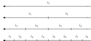
Fig. 2.Haar wavelet MRA of the 2πangular domain. Each spaceVlhas 2lsubdivisions.

Fig. 3.ExampleofHaarwaveletsonaquadrantofthe2πangulardomain.EachVjspace(denotedontheleft)isreproducedbyVj=Vl⊕nj−=12Wn(denoted ontheright).SpaceV5canbethusreproducedbyV5=V2⊕W2⊕W3⊕W4.

TheHaarwaveletsaredefinedas

ψ

n,k

(x)

=

⎧

⎪

⎨

⎪

⎩

1 ifx

∈

i2k−1

,

−

1 ifx

∈

i2k

,

0 otherwise

,

(33)

wheren

∈ {

l

,

l

+

1

,

. . . ,

j

−

1

}

forVj.ThehierarchyofscalingfunctionsandwaveletsispresentedinFig. 3.First,thescaling

functionsare expandedon Vl.Onthefirstwaveletlevel,Wl,waveletsspanthesamespaceasthescalingfunctionsinVl.

Foreverynewlevelthenumberofwaveletsdoublesandthuseachnewwaveletsupportshalfthespace.

If(32)and(33)aresubstitutedinto(31),theHaarwavelets’approximationforanyfunctioninL2

(

R

)

becomes,

f

(x)

≈

2l

k=1

α

k

φ

l,k

(x)

+

j−1

n=l 2n

k=1

β

_n,k

ψ

n,k

(x).

(34)

Equation(34)showsthatanyfunctioninL2

₍

R

)

canbeapproximated,withalinearcombinationofthescalingfunctions on levell andthewavelets onlevels n

∈ {

l

,

l

+

1

,

. . . ,

j

−

1

}

. Henceforth,theHaar waveletdiscretisation isreferred to as HWl,j.Following(28),

HWl,j

=

Vl

⊕

Wl

⊕

Wl+1

⊕

....

⊕

Wj−1

=

Vj

.

(35)

HW2,5 forinstancehas22 scalingfunctionsin V2,22 waveletsin W2,23 waveletsin W3 and24 waveletsinW4.The

resultingspaceisV5 withacumulativenumberoffunctionsequalto25

=

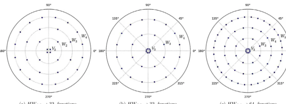
32 (Fig. 3).Tovisualisetheangularmesh,polar

plotsareusedthatshowthepositionofthefunctions(middlepoint)forallthelevels(Fig. 4).

3.4. Calculatingtheangularmatrices

Equation(34)provides an expressionforrepresenting afunction withHaarwavelets.Assuming thelevels ofthe scal-ing functionsandwaveletsare known,the numberoffunctionsusedfor theprojection isalso known.Then (34)can be condensedtothesinglesummationgivenin(7):

N(r

,

t, θ )

≈

K

j=1

[image:8.561.188.351.166.326.2]

[image:9.561.47.504.52.219.2]

Fig. 4.Polar plots for various Haar wavelet expansions. Each concentric circle represents the spaces:{Vl,Wl,Wl+1, . . . ,Wj−1}, for aHWl,jdiscretisation.

where Nj corresponds to thecoefficients

α

,

β

and Gj tothefunctions

φ

and

ψ

of(7). Thus,scaling functionsandHaar

wavelets arenow simplyreferred to asangularbasisfunctions. Havingtheapproximation fortheangular dependenceof the actiondensity,allthatisneededfortheimplementationofHaarwaveletsistocalculatetheangularmatricesAx,Ay,

M,Hθ of(13)–(16),presentedinsection2.2.

Thevastmajorityoftheavailablespectralwavemodels,useafinitedifferenceapproximationfortheangulardimension. Thisistheequivalentofacellcentredfiniteelement P0 discretisation.IntheBoltzmanntransportcommunitythisisknown as discrete ordinates or SN [36]. If the angular matrices are calculated forthis expansion then there exists a mapping operator

W

, which maps the P0 space to the Haar space (both are piecewise constant, so the mapping is exact). The relationshipis

W

_NW

=

NP0

,

(37)

where NW andNP0 correspondtotheactiondensityapproximatedinthewaveletspaceandthe P0 finiteelementspace

respectively. This mapping is applied to the angular matrices by pre-multiplying and post-multiplying by

W

T and

W

respectivelyas,

AW_x

=

W

T_AP0

x

W

.

(38)

The mappingmatrix

W

isasquare matrixof1’s,

−

1’s and0’s.Theuseofthemappingoperator simplifiesthe imple-mentation ofHaarwavelets,allowingthemtobe builtonexisting conventionalframeworks.Thisisparticularlyusefulfor thecalculationofthesourceterms(whicharenotincludedinthisstudy).

4. Angularadaptivity

The applicationof anisotropic angularadaptivity, i.e. allowing the model to use a different angular discretisation for each spatial node, wouldnormally requirethe reconstruction of the angularmatrices (13)–(16) foreach spatial node at each adaptive time-step. This can be a cumbersome task with a significant computational cost. Fortunately, the whole processcanbeeasilysimplifiedwiththeuseofhierarchicalexpansions,suchastheHaarwaveletsusedhere.Tomakethis clear,assume thatauniformexpansionisappliedglobally.Thecoefficientsofthisexpansionwillbehighatspatial nodes where theactiondensityis high,andlow inareas oflowaction density.As thesecoefficientsgetsmallera filtercanbe appliedtozerothemoutandeventuallyremovethemfromtheexpansion.Thisisknownasthresholdingandusedfordata compression[41].

Applyingthisonanadaptiveframework,theangularmatricesarecalculatedforauniformexpansion,andforeachspatial node onlythecoefficientsthatareabovethethresholdareaddedtothefinalsystem.Thisiswheretherealbenefitsfrom theuseofHaarwaveletscanbeseen,duetotheircompactsupport;everytimeanewlevelgetsaddedthesupportofthe waveletsbecomessmaller,focusingonmoredetailintheangulardomain.Thus,anadaptiveschemewithwavelets,allows fortheconcentrationofanglesonspecificpatchesoftheangulardomainforeachspatialnode.Thiscansignificantlyreduce the total numberofbasis functions. An added benefitoftheir hierarchical natureis that thereis no needto interpolate between consecutiveangularmeshes. Projectingone adapted angularmesh ontothe next simplyconsists ofcopying the existingangularcoefficientsovertothenewangularmesh.

[image:10.561.158.381.55.108.2]

A. Adam et al. / Journal of Computational Physics 305 (2016) 521–538

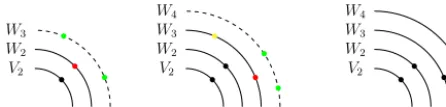
Fig. 5.Simplifiedexampleoftheangularadaptivescheme.Startingfromtheleftsketchtheredbasisfunctionsuggeststhattherespectivenextlevel(dashed line)basisfunctions(green)shouldbeadded,i.e.thewaveletcoefficientisbiggerthanthetoleranceNi>τ.Thecentralsketchshowsthatoneofthetwo newlyaddedbasisfunctionscanberemoved(yellow),whiletheotherrequiresyetanotherlevel.Thesketchontherightshowsthefinaladaptedsystem. (Forinterpretationofthereferencestocolorinthisfigurelegend,thereaderisreferredtothewebversionofthisarticle.)

4.1. Errormeasure

Haarwaveletsprovideanaturalframeworkforidentifyingtheregionswheretheactiondensityisunder- orover-resolved andhencethecomputationalresolutionshouldbealtered. Eachwaveletcoefficientgetssmallerasitsimportancebecomes smaller.Thus,amagnitude-basederrormetriccanbedefinedtoindicatewhetherawaveletcoefficientissufficientlysmall toberemoved,orsufficientlylargeforitshigherlevelhierarchicalwaveletstobeadded.Asimplifiedexampleispresented inFig. 5.

Buchanetal.in[39]suggestthatanappropriateerrormetrictobeusedisNjGjAj whereNj istheangularcoefficient,

Gj the basis function and Aj the supportarea ofthebasis function. However, forthe Haar waveletsthe basis functions

switch between1 and

−

1 and,aftersomeinitial results,theintroductionofthearea didnot appeartohaveasignificant impact.Thus,theerrormetricisimplementedas

Ni

>

τ

.

(39)

Iftheangularcoefficientisgreaterthanauser-definedtolerancevalue

τ

thentheerrorisconsideredsignificant, suggest-ingthatmoreresolutionshouldbeaddedtothisregion,i.e.waveletsfromthenextlevelshouldbeincluded.Thiscouldbe repeateduntilenoughlevelshavebeenadded,suchthatnoneofthevaluesfor Ni arebiggerthan

τ

.However,inpractice

itisbettertorestrictthemaximumnumberoflevels.Thismeansthatboth aHWl,jinit andaHWl,jmax are defined,forthe

initialandfinestpossiblediscretisationrespectively.

Finallyawaytoremovebasisfunctionsisalsoneededtoensurethattherearenoover-resolvedregions.Thisthreshold issetto Nj

<

0

.

01

τ

;everytime anangularcoefficientissmallerthan0

.

01

τ

itisremoved.Thisdoesnot applytoscaling

functions.

4.2. Adaptiveprocedure

Theoveralladaptiveprocedurecanbedescribedas,

1. StartwithaHWl,jinit discretisation,choosethemaximumvalue jmax andatolerancevaluefortheerrormetric

τ

(39).

2. Runthenon-adapted HWl,jinit system.

3. Loopeveryangularcoefficient Niforeveryspatialnodeandevaluateiftheyarewithintheerrorbounds,

if Ni

/

τ

>

1

→

If not at max level, add the next level functions forNi

,

if Ni

/

τ

<

0

.

01

→

If not a scaling function, removeNi

,

if 0

.

01

≤

Ni

/

τ

≤

1

→

KeepNi

.

4. Reassemblethesystemmatrices(section2.4),butonlyadd thecomponentsoftheangularmatrices,correspondingto theadaptedangularcoefficients.

5. For stationarysimulations, repeat the above process until convergence (i.e. the algorithm has stopped changing the angularmesh),oramaximumnumberofadaptshasbeenreached.

6. Fornon-stationaryapplications,chooseanadaptperiodtospecifyatwhichtime-stepstheadaptivityalgorithmwillbe evoked.

Owingto theSGSmethod(section2.4),theaction densityisdiscontinuous. Thesystemthat getsassembled,however, iscontinuous. Acontinuous errormetricis,thus, necessarytoapply tothe adaptivealgorithm.Onewayto derivethisis by looping overthe elements containing the samenodes andkeepingthe maximum values.Even though the frequency discretisation is omitted in this study, it is worth mentioning that in the case of multiple frequency groups a similar approachcan beusedto getasingle errorvalueforall groups. Thefrequencygroupsareloopedoverandthemaximum valuefortheactiondensityiskeptfortheerrormetric.

Finally a note on the use of the scaling functions. Given that HW2,5 andHW3,5 both result in the same numberof

[image:11.561.148.400.53.191.2]

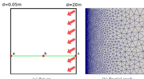
Fig. 6.Depthinducedshoalingandrefraction.Set-upexplanationandspatialmesh.(Forinterpretationofthereferencestocolorinthisfigure,thereaderis referredtothewebversionofthisarticle.)

theadaptivealgorithmcannotremove;thusbychangingl,theminimumnumberofbasisfunctionscanbeeasilycontrolled givinganextradegreeoffreedomintheadaptiveprocedure.Thiscouldproveimportantintransientsimulationswhenthe wave field changes abruptly.The adaptivealgorithm mightnot haveenough time toresolve theseareasanda minimum numberoffunctionscouldbenecessarytoprovideanaccuraterepresentation.

5. Numericalresults

To present the adaptive framework and attempt to quantify its benefits two test cases are selected. The first one is a stationary depth-induced shoaling and refractiontest case, routinely used to benchmark spectral wave models. This is a highly directional problem, where the angularresolution dominates theerrors. The second is an idealised deep water propagation scenario which isa standard test case forstudying the“Garden Sprinkler Effect” (GSE). The GSE is a direct result oftheangular discretisationand thushighly sensitive to theangularresolution. Sinceno effort hasbeen spent to optimise thecode,theresults arenot comparedagainst otherspectral wave models.InsteadHaar adaptivityis compared againstuniformresolutionswithinthesamecodetodemonstratetheadvantagesoftheproposednumericalframework.

5.1. Depth-inducedshoaling-refraction

A plane beach front is considered, represented by a 4000 m

×

4000m domain, with a bathymetric slope of1

:

200. A long waveenters fromthedeepeastern boundarywithd

=

20m,atanangleof210◦ (measuredcounter-clockwisefor thepositivex-axis),propagatingtowardstheshallowwesternboundarywithd

=

0

.

05m (Fig. 6(a)).Asthewaveencounters shallowerwaters, itslowsdown,causingits wave lengthtodecrease and,thus, itswave height toincrease (shoaling).To account forthis,the spatialmeshhasa variableelementsize,starting fromanedge lengthof600m and goingdown to 20m (Fig. 6(b)).Asdifferentpartsofthewave-traintravelwithdifferentspeeds,thewavealsoturns(refraction).

Totest shoalingandrefraction,a monochromaticwave isset-upwithasignificant waveheight of1m,afrequencyof 0

.

1Hz anda cos500

_{(θ )}

_{directional distribution(thisresultsin adirectional widthof}

_σ

θ

=

2

.

5◦,where

σ

θ isthe standard

deviationofthedirectionaldistribution[47]).Thesignificantwaveheightandtheangleofdirectioncanbecomparedto,

H2 H2_i

=

cgicos

(θ

i

)

cgcos

(θ )

,

(40)

sin

(θ )

sin

(θ

i

)

=

c

ci

,

(41)

where H is the significant wave height,

θ

is the direction, cg and c the group and phase velocity respectively, while i

denotestheincidentvalue.

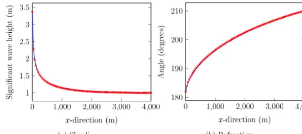
Firstthe P0 angulardiscretisationistestedwith400 angulardegreesoffreedom

(θ

=

0

.

9◦

)

.Theresultsofthe simu-lationplottedalongthe y

=

1000m line(greenlineofFig. 6(a))arepresentedinFig. 7,showinggoodagreementforboth shoalingandrefraction.

ArefractionconvergencetestfortheuniformP0angularmeshispresentedinFig. 8.Foreachsimulationthenumberof anglesisdoubledandthediscreteroot-mean-square(RMS)errorplotted,comparedto(41),alongthey

=

1000m line.This is presentedby thebluelineinFig. 8,wherefirstorderconvergence

(

p

+

1

)

isachieved. Inthesesimulations,the angles areuniformlyappliedtoallthespatialnodesofthedomain.Howeverthedirectionalwidthisnarrowwhichmeansthatas theangularmeshisrefined,averysmallnumberoftheangleshaveanon-zeroactiondensity.

[image:12.561.121.420.55.188.2]

A. Adam et al. / Journal of Computational Physics 305 (2016) 521–538

Fig. 7.Validationfordepthinducedshoalingandrefraction.AP0 angulardiscretisationwith400 anglescomparedagainsttheanalyticalsolutions of(40)and(41).

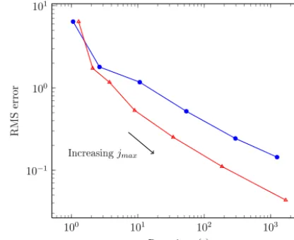
Fig. 8.Depthinducedrefraction.ConvergencetestsforuniformP0 andHW3,j, jmax∈ {4,5,6,7,8,9,10},adaptivediscretisationsforvarious

toler-ances:τ=1 ,τ=10−1 _,τ=10−2 _.TheHW

3,jpointscorrespondtotheresultsaftertheadaptivealgorithmconverges.(Forinterpretation ofthereferencestocolorinthisfigure,thereaderisreferredtothewebversionofthisarticle.)

theangularmeshandthereisnochangeintheactiondensity.Thiswaythecomputationalcostsaresmallandonlygrow according to the errors of the simulation.In practice the convergence criteria should be relaxed to a percentage ofthe changeoftheactiondensity(orthesignificantwave height),asafterapointthechangeintheactiondensitywillbe too smalltojustifytheextracostofre-runningthesystem.

For each HWl,j simulation the scaling function and initial levels are jinit

=

l

=

3. The maximum level jmax is

in-creased and the RMS error is plotted, compared to (41), along the y

=

1000 m line. The results for a HW3,j, jmax

∈

{

4

,

5

,

6

,

7

,

8

,

9

,

10

}

,discretisationwithtolerances

τ

∈ {

1

,

10−1

,

10−2

}

arepresentedinFig. 8.

Foratolerance

τ

=

1,as jmax increasestheerrorsappeartolevelout. Asnewlevelsareintroduced,the valuesofthe

action densitycoefficients Ni become smaller,until they are ignored by the adaptive algorithm.Thus, even though jmax

increasesthereisnotenoughresolutionto representthedirectionaldistributionoftheactiondensityandtheerrorsstop decreasing.This isa clearindication that theselected tolerancevalue is toolarge. Decreasing the toleranceto

τ

=

10−1

amendsthisandproduces errorscomparabletotheuniformresolutiondiscretisation.Afurtherreductionofthetolerance to

τ

=

10−2 _{produces similar errors to}

_τ

₌

₁₀−1_{,with a higher numberof angular basis functions. This means that as}

thetoleranceisfurther decreased,newbasis functionsare introducedthat donothaveasignificant impactontheerrors ofthe simulation.Indeed, foran infinitesimal value of

τ

adaptivity shoulduniformly add all theangular basis functions producingthe sameresultsastheuniform P0 discretisation.It isthe balancebetweenaccuracyandcomputational costs thatultimatelydefinesthetolerancevalue.

In terms ofthe computational degrees offreedom, the adaptive HW3,j discretisations consistently use fewer degrees

offreedomcomparedtothe uniformP0 discretisations.Theerrorlevelfora P0 angulardiscretisationwith128 anglesis achievedwithalmostanorderofmagnitudelessdegreesoffreedombytheadaptiveHW3,7 discretisation.Movingtowards

finerangular meshes,thisdifference becomes evenbigger,showing theadvantages ofangularadaptivity forhighfidelity results.

To seehow this translatesin computational times,the results witha tolerance

τ

=

10−1 _{are isolated and theerrors}

[image:12.561.165.372.225.394.2]

[image:13.561.171.379.57.227.2]

Fig. 9.Depthinduced refraction.Convergencetests foruniform P0 with {16,32,64,128,256,400}angles and HW3,j, jmax∈ {4,5,6,7,8,9,10}, adaptivediscretisationsforatoleranceτ=10−1 _.TheHW

3,jpointscorrespondtotheresultsaftertheadaptivealgorithmconverges.

Fig. 10.Polar plots for aHW3,10discretisation for points:a=(0 m,1000 m),b=(2000 m,1000 m),c=(4000 m,1000 m)inFig. 6(a).

levels adaptive HW3,j discretisationsrun consistentlyfaster, withdifferencesapproaching an orderofmagnitude forfine

resolutions.Fortheuniform P0 angulardiscretisationwith128 angles,thesameerrorisachievedbytheHW3,7,sixtimes

faster. Itisworthnotingthatthe HW3,7 convergesaftertenadapts,i.e.solvingtentimestheadapted systemissixtimes

fasterthansolvingtheuniformsystemonce.

FinallyinFig. 10thepolarwaveletplotsforaHW3,10discretisationwithatoleranceof

τ

=

10−1arepresentedforthree

differentlocationswithcoordinates:

(

0m

,

1000m

)

,

(

2000m

,

1000m

)

,

(

4000m

,

1000m

)

,orpointa,b andc inFig. 6(a). As thewave propagatesfrompoint c topointa,its meandirectionshiftsfrom210◦ to 180◦.The angularbasisfunctions follow thechangeof themeandirectionrefining onlythe patches oftheangulardomain that areactive foreach spatial node.

5.2. Deepwaterpropagation

An inherent problemof the phase-space discretisation is the spurious separation of energy intothe discretised bins. This is called the “Garden Sprinkler Effect” and has been extensively studied in [48,49,20]. (In the Boltzmann trans-port community this is known asthe ray effect.) To showcase thiseffect in the angular dimension, a large spatial do-main

(

4000km

×

4000 km

)

is simulated, witha monochromatic wave propagating over a long distance in deep water (d

=

10000 m). Forthe spatial discretisation a structured trianglemesh isused, withan element edge length of67 km (Fig. 11(a)).Theinitial wavefield,located 500km fromthelower andleft sidehasaGaussian distributioninspace,with a significant wave height of Hs

=

2

.

5m and a standard deviationof150km (Fig. 11(b)).Its meandirectionis 30◦ with

an angulardistributionofcos2

_{(θ )}

_{andafrequencyof0}

_.

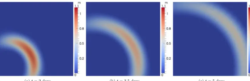
_{1Hz.Thesimulationistime-dependent andrunsfor5dayswitha}

[image:13.561.42.504.267.438.2]

[image:14.561.124.418.52.202.2]

A. Adam et al. / Journal of Computational Physics 305 (2016) 521–538

[image:14.561.48.493.238.379.2]

Fig. 11.Spatial mesh and initial conditions for the deep water propagation test case.

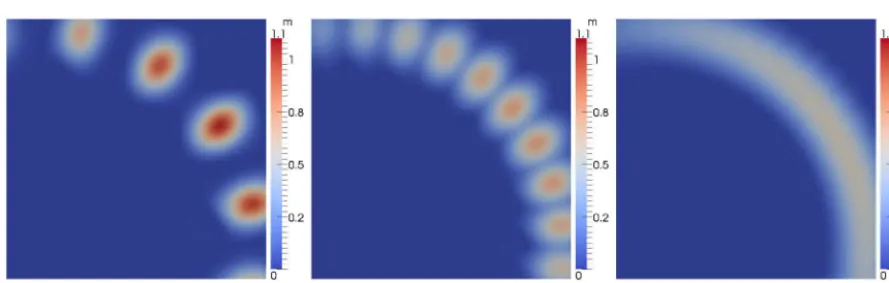
Fig. 12.Significant wave height after 5 days of deep water propagation, for aP0 angular discretisation with various angular resolutions.

In Fig. 12, the results at the final timestep for a P0 angular discretisation with 16, 32 and 64 basis functions are presented.As thewave propagates, it breaks up intothe pathsof theprescribed directions; thecoarser theangular dis-cretisation,themoreintensetheGSE willbe.Thisisalsoconnectedtothenumericaldiffusionofthespatialdiscretisation. Higher orderschemeshavea lower numericaldiffusion,whichintensifiestheGSE. Thisessentiallymeans that increasing theresolutioningeographicspacemakestheGSEworse.

The obvioussolution isto increase the numberof angles.However, in themultidimensional framework ofthe action balanceequationincreasingthenumberofanglesgloballysignificantlyaffectsthecomputationalcosts.Withafiniteelement expansion,astheonepresentedhere,doublingtheangularbasisfunctionsquadruplesthesizeoftheangularmatrices.This increased computational cost for finer angular resolutions, led to the use of a diffusion correction termby [48], which smearsouttheactiondensitydependingonthewaveage.Byknowinghowmuchthewavefieldhaspropagated,itcanbe spreadaccordinglytoalleviatetheGSE.Calculatingthewaveage,however,iscostly,leavingtheageasatunablecoefficient, whichintroducesinaccuracies.

Here,asan alternative,angularadaptivityisused,toincreasetheaccuracyofthesolutionwhilekeepingthe computa-tionalcostataminimum.AHW2,6discretisationisapplied,withatolerancevalueof

τ

=

10−6.Thisintroducesamaximum

of26

=

64 basisfunctions,makingtheresultscomparabletotheuniformP0 with64angles.Bystartingthesimulationsat thescalingfunctionlevel,asinthestationaryexample,theinitialcos2

(θ )

distributionisonlyrepresentedby4 angles.This ofcourseintroduces errorswhichthenpropagate throughoutthesimulation.Thus, thesimulationstartsatthemaximum angulardiscretisation jinit

=

jmax.(Analternative wouldhavebeen tobe able toadapt afew timesat thefirst timestep

beforepropagatingintime.) Giventhatthecostofadaptingisnegligible,adaptivityisactivatedateachtime-step.

InFig. 13theadaptiverunispresentedatvarioustimelevels,whileFig. 14showsthedifferencebetweenthesignificant waveheightfortheHW2,6andP0

−

64 anglesruns.Theresultsarereadilycomparable,withdifferencesintheorderof mm.

However, capturing the solutionis only partof the goal,as theobjective is the reduction ofthe computational cost. Toshowcasethis, theangularmesh,orthedistributionofthenumberofangularbasisfunctionsinspace,ispresentedin

[image:15.561.58.496.56.198.2] [image:15.561.54.492.226.372.2]

Fig. 13.Significant wave height for an adaptiveHW2,6discretisation with toleranceτ=10−6at several time levels.

Fig. 14.AbsolutedifferenceinsignificantwaveheightbetweenaP0−64 angleandanadaptiveHW2,6discretisationwithtoleranceτ=10−6forvarious

timelevels.Colorbarinlogarithmicscale.

Fig. 15.Angularmesh,i.e.numberofangularbasisfunctions,foraHW2,6discretisationwithtoleranceτ=10−6atvarioustimelevels.Thepolarplotsfor

thepointsdenotedbytheyellowdotsarepresentedinFig. 16.(Forinterpretationofthereferencestocolorinthisfigurelegend,thereaderisreferredto thewebversionofthisarticle.)

Finally in Fig. 16the polar plots forthe three geographical points denoted by the yellowdots inFigs. 15(a)–(c), are presented at their respective time levels. For each point, the wave field has a different mean direction anddirectional distribution.Adaptivityadjuststhenumberandpositionofangularbasisfunctionsaccordingly.

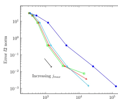
Tobetterquantifythesavingsinthecomputationalcosts fromusingangularadaptivitya convergencetest isnow pre-sented. Firstthe P0 angulardiscretisationistested.With300anglesusedtoconstructthereferencesolution,thenumber ofanglesisgraduallyincreasedandthel2 normofthesignificantwaveheightforthefinal timestepisplottedagainstthe run-time.ThisispresentedinthebluelineofFig. 17.

Fortheadaptedruns,aHW2,j, jmax

∈ {

3

,

4

,

5

,

6

,

7

,

8

}

,discretisationisusedwithtolerances

τ

∈ {

10−6

,

10−7

,

10−8

}

.The

[image:15.561.56.498.409.552.2]

[image:16.561.38.503.51.217.2]

A. Adam et al. / Journal of Computational Physics 305 (2016) 521–538

Fig. 16.Polar plots of aHW2,6discretisation for the points inFig. 15, at their respective time levels.

Fig. 17. Erroragainstrun-timefor thedeepwater propagationtestcase.Results for P0 with{8,16,32,64,128,256}angles and HW2,j, jmax∈ {3,4,5,6,7,8},fortolerances:τ=10−6 _,τ=10−7 _,τ=10−8 _{.Eachpointcorrespondstotheerrorcomparedtoauniform}

P0 discretisation with300 angles,atthefinaltimelevel.(Forinterpretationofthereferencestocolorinthisfigure,thereaderisreferredtothewebversionofthisarticle.)

linesmovetowardshigherrun-timesandsmallererrors.Usingasmallertolerancevalue,adaptivityinsertsmoreanglesand thustherun-timesarehigher.However,upto jmax

=

7 theerrorsarethesameforalltolerances,i.e.theextraangularbasis

functionsthatareinserteddonotsignificantlyimpacttheerror.Asignificantdifferencecanonlybeseenforthelast value of jmax

=

8.Thisisthepointwheretheaccuracyofthesolutioniscomparabletothetolerancelimitandthusdecreasing

thetolerance producesbetter results.Forthe caseof

τ

=

10−8 _{the highestvalue of j}

max

=

8 givesthe sameerrorvalues

astherespectiveuniform P0 runs.Thisisausefulguidetohowthetoleranceshouldbe tuneddependingonthedesired accuracy.

Theadaptivesimulationsareconsistentlyfastercomparedtotheuniformresolutionones.Thesameerrorproducedbya uniform P0 angulardiscretisationwith128 anglesisachievedalmostanorderofmagnitudefasterby theHW2,7 adaptive

discretisation. As the angular resolutions increase this difference becomes bigger. This is dueto the reduced numberof degreesoffreedom,asisevidentinFig. 18,wherethemeannumberofangularbasisfunctionsforatoleranceof

τ

=

10−6 is plottedateach time level.At thefirst time level,the simulationstarts withthe maximumnumberof anglesso asto accuratelyrepresenttheinitial angulardistribution.Afterthefirstadapt,themeannumberofbasisfunctionsimmediately dropsandthesimulationsrun consistentlywithuptoanorderofmagnitudefewerdegreesoffreedom.Asthewave field propagates it spreads covering a larger computational area. Thus, the degrees of freedom increase towards higher time levels, onlyto decrease againwhen partsof thewave field exitthe domain.This constant adjustmentofthe degreesof freedomensuresthatthecomputationalcostsarealwaysoptimiseddependingonthedesiredaccuracy.

6. Conclusions

[image:16.561.167.372.243.414.2]

[image:17.561.167.382.51.231.2]

Fig. 18.Meannumberofangularbasisfunctionsagainsttimelevelforthedeepwaterpropagationtestcase.HW2,3 ,HW2,4 ,HW2,5 ,HW2,6

,HW2,7 ,HW2,8 ,foratoleranceofτ=10−6.

ofanglesused needstobe keptsmall.Ingeneral, however,seasurfacewind-wavefieldsaredirectionalandthusinmost casesthemajorityofangulardegreesoffreedomdonotsignificantlyimpactontheaccuracyofthesolution.Whatismore, the meandirectionofthewave fieldisconstantlychanging andtherateofthischangeissubjecttoexternal forces,such as the wind, currents andthe bathymetric slope. Hence, a-priori estimation of the required angular mesh resolution is challenging.

Toresolvethisproblem,thispaperintroducesanewframeworkforapplyingangularadaptivityinspectralwavemodels. Themethodemployshierarchicalangularexpansions,usingHaarwaveletstorepresenttheangulardependenceoftheaction density.Theadaptiveprocedureusesthehierarchyandcompactsupportofwaveletstolocatetheareasontheangularmesh thatareunder-resolvedandincreasethenumberofangularfunctionstolocallyrefinetheresolution.Atthesametime,areas that areover-resolvedare identifiedandfunctionsremovedto decreasetheglobaldegreesoffreedom withoutnegatively impacting ontheaccuracy.Bycontrollingtheminimumandmaximumnumberofbasisfunctions,aswellasthetolerance fortheerrormetricthebalancebetweenerrorsandcomputationalcostsiseasilymanaged.

The methodis appliedto a steadystate depthinduced shoaling-refraction testcase, aswell asa transient largescale propagationtestcase.Theadaptiveresultsareverifiedagainstauniformresolutiondiscretisationandthegainsintermsof computationaldegreesoffreedomandrun-timesarequantified.

Waveletsareconstantlyrearrangedforeachgeographicpointfollowingthemeandirectionandcapturingthedirectional distributionofthewavefield.Thus,thesameerrorlevels,comparedtoauniformexpansion,areachievedinbothcaseswith lowercomputationalcostsandfasterruntimes.Inparticular,foranangularresolutionof128 angles,adaptivityrunswithan orderofmagnitudelessdegreesoffreedomcomparedtotheuniformresolution.Thistranslatesinsixtimesfasterrun-times fortheshoaling-refractiontestcaseandalmostanorderofmagnitudefasterruntimesforthelargescalepropagationtest case.Thisreferstothetotalrun-timesincludingboththelinearsolvesandtheadaptprocess.Thedifferencewidensasthe angularmeshisfurtherrefined,showingtheadvantageofadaptivityforhighfidelityresults.

Inalltheresultspresentedtheobjectiveistoshowthatadaptivewaveletscanreproducethesameerrorsasthe equiv-alentuniformresolutionangularmeshes.Thus,theconvergencecriteriaarestrictandthetolerancelimitslow.Inpractical simulations the convergencecriteriaandtolerance limitsneedto be linked tothe changeofthe significant wave height, whichwillresultinfewerangularbasisfunctionsand,thus,fasterrun-times.Speed-upscanalsobeachievedbyoptimising thescheme,suchasexploitingthesparsityoftheangularmatricesforthemapping.

Haar wavelets providean effectiveframework forapplying anisotropic angularadaptivity,refining the angular resolu-tion according tothe desiredaccuracy while atthe sametime reducing thecomputational costs. This can pushspectral wave modelstowardshigherresolutionsandhelpbridgethegapbetweencoarselargescaleandfinecoastalzone simula-tions.

Acknowledgement

A. Adam et al. / Journal of Computational Physics 305 (2016) 521–538

Appendix A. Sub-gridscalematrices

Thesub-gridscalematrices

A

_,

B

_,

C

_,

D

,are,

A

_i,j

=

V

PiM

1

t

PjdV

+

V

PiHθ

(

r

)

t,σPjdV

+

V

PiHf

(

r

)

t,σ

1

fPjdV

+

Ŵ Pi

Acg

(

r

)

t,σ

+

Mu

(

r

)

t,σ

·

n

PjdŴ

−

V

∇

Pi

·

Acg

(

r

)

t,σ

+

Mu

(

r

)

t,σ PjdV (A.1)

B

_i,j

=

V

PiM

1

t

QjdV

+

V

PiHθ

(

r

)

t,σQjdV

+

V

PiHf

(

r

)

t,σ

1

fQjdV

−

V

∇

Pi

·

Acg

(

r

)

t,σ

+

Mu

(

r

)

t,σ QjdV (A.2)

C

_i,j

₌

Ve

QiM

1

t

PjdV

+

Ve

QiHθ

(

r

)

t,σPjdV

+

Ve

QiHf

(

r

)

t,σ

1

fPjdV

+

Ve

Qi

Acg

(

r

)

t,σ

+

Mu

(

r

)

t,σ

· ∇

PjdV

+

Ve

Qi

∇ ·

Acg

(

r

)

t,σ

+

Mu

(

r

)

t,σ PjdV (A.3)

D

_i,j

₌

Ve

QiM

1

t

QjdV

+

Ve

QiHθ

(

r

)

t,σQjdV

+

Ve

QiHf

(

r

)

t,σ

1

fQjdV

+

Ŵe_out

Qi

Acg

(

r

)

t,σ

+

Mu

(

r

)

t,σ

·

n

QjdŴ

−

Ve

∇

Qi

·

Acg

(

r

)

t,σ

+

Mu

(

r

)

t,σ QjdV (A.4)

Si

=

ηQ

j=1

V

NiSjQj (A.5)

S _i

=

ηQ

j=1

V

QiSjQj (A.6)

wherei, jcorrespondtoblockmatricesofsize K

×

K,i.e.theycontaintheangulardiscretisedinformationoneachspatial node.Theintegral

Ŵout

d

Ŵ

referstotheoutgoingcomponentoftheboundaryintegral

Ŵ

d

Ŵ

.

References

[1]J.A.Battjes,Shallowwaterwavemodeling,in:M.Isaacson,M.Quick(Eds.),ProceedingofInternationalSymposiumWaves–PhysicalandNumerical Modeling,UniversityofBritishColumbia,Vancouver,ASCE,1994,pp. 1–23.

[2]W.J.Pierson,G.Neumann,R.W.James,PracticalMethodsforObservingandForecastingOceanWavesbyMeansofWaveSpectraandStatistics,H.O. Pub.,vol. 603,USNavyHydrographicOffice,1955.

[3]R.Gelci,H.Cazalé,J.Vassal,Prévisiondelahoule.Laméthode desdensitésspectroangulaires,Bull.Inf.ComitéOcéanogr.EtudeCôtes9(1957)416–435.

[4]L.H.Holthuijsen,WavesinOceanicandCoastalWaters,CambridgeUniversityPress,2007.

[5]SWAMPGroup,OceanWaveModeling,PlenumPress,1985.

[6]WAMDIgroup,TheWAMmodel—athirdgenerationoceanwavepredictionmodel,18(1988)1775–1810.

[7]G.B.Whitham,LinearandNonlinearWaves,AWiley–IntersciencePublication,Wiley,1974.

[8]P.A.E.M.Janssen,Progressinoceanwaveforecasting,in:PredictingWeather,ClimateandExtremeEvents,J.Comput.Phys.227 (7)(2008)3572–3594.

[9]L.Cavaleri,J.H.G.M.Alves,F.Ardhuin,A.Babanin,M.Banner,K.Belibassakis,M.Benoit,M.Donelan,J.Groeneweg,T.H.C.Herbers,P.Hwang,P.A.E.M. Janssen,T.Janssen,I.V.Lavrenov,R.Magne,J.Monbaliu,M.Onorato,V.Polnikov,D.Resio,W.E.Rogers,A.Sheremet,J.McKeeSmith,H.L.Tolman,G. vanVledder,J.Wolf,I.Young,Wavemodelling–thestateoftheart,Prog.Oceanogr.75(2007)603–674.

[10]H.L.Tolman,Athird-generationmodelforwindwavesonslowlyvarying,unsteady,andinhomogeneousdepthsandcurrents,J.Phys.Oceanogr.21 (6) (1991)782–797.

[11]N.Booij,R.C.Ris,L.H.Holthuijsen,Athird-generationwavemodelforcoastalregions:1.Modeldescriptionandvalidation,J.Geophys.Res.104 (C4) (1999)7649–7666.