Trade Liberalization, Intermediate Inputs, and Productivity: Evidence from Indonesia

1942

Importers

,

Exporters

,

and Exchange Rate Disconnect

By Mary Amiti, Oleg Itskhoki, and Jozef Konings*

Large exporters are simultaneously large importers. We show that this pattern is key to understanding low aggregate exchange rate pass-through as well as the variation in pass-through across exporters. We develop a theoretical framework with variable markups and imported inputs, which predicts that firms with high import shares and high market shares have low exchange rate pass-through. We test and quantify the theoretical mechanism using Belgian firm-product-level data on imports and exports. Small nonimporting firms have nearly complete pass-through, while large import-intensive exporters have pass-through around 50  percent, with the marginal cost and markup channels contributing roughly equally. (JEL D24, F14, F31, L60)

One of the central puzzles in international macroeconomics is why large move-ments in exchange rates have small effects on the prices of internationally traded goods. This exchange rate disconnect has generated a vast literature, yet no empiri-cal pass-through study has taken into account one of the most salient features of international trade, that is, that the largest exporters are simultaneously the largest importers. In this paper, we show that this pattern is key to understanding the low aggregate pass-through, as well as the variation in pass-through across firms.

Using detailed Belgian micro data, we find that more import-intensive export-ers have significantly lower exchange rate pass-through into their export prices, as they face offsetting exchange rate effects on their marginal costs. These data reveal that the distribution of import intensity among exporters is highly skewed, with the import-intensive firms being among the largest exporters, accounting for a major share of international trade. Consequently, the import-intensive firms also have high export market shares and hence set high markups and actively move them in response to changes in marginal cost, providing a second channel that limits the

* Amiti: Federal Reserve Bank of New York, 33 Liberty Street, New York, NY 10045 (e-mail: [email protected]. org); Itskhoki: Department of Economics, Princeton University, Princeton, NJ 08544 (e-mail: itskhoki@princeton. edu); Konings: Department of Economics, University of Leuven, Naamsestraat 69, 3000 Leuven, Belgium, National Bank of Belgium, and Department of Economics, University of Ljubljana, Slovenia (e-mail: [email protected]). We gratefully acknowledge the National Bank of Belgium (NBB) for the use of its research facilities and data, and in particular Valere Bogaerts for help with the data collection, and Emmanuel Dhyne, Catherine Fuss, and Raf Wouters for comments and data clarifications. We thank George Alessandria, Ariel Burstein, Elhanan Helpman, Doireann Fitzgerald, Linda Goldberg, Logan Lewis, Nick Li, Ben Mandel, Ulrich Müller, Steve Redding, Esteban Rossi-Hansberg, David Weinstein, Hylke Vandenbussche, and seminar participants at multiple venues for insightful comments. We also thank Sydnee Caldwell, Stefaan Decramer, Cecile Gaubert, Diego Gilsanz, Preston Mui, and Mark Razhev for excellent research assistance. The views expressed in this paper are those of the authors and do not neces-sarily represent those of the Federal Reserve Bank of New York or the NBB. The paper uses confidential data provided by the NBB. The NBB had the right to review the paper prior to its circulation.

effect of exchange rate shocks on export prices. These two mechanisms reinforce each other and act to introduce a buffer between local costs and international prices of the major exporters, thus playing a central role in limiting the transmission of exchange rate shocks across countries. The availability of firm-level data with imports by source country and exports by destination, combined with domestic cost data, enables us to estimate the magnitude of these two channels.

To guide our empirical strategy, we develop a theoretical framework to study the forces that jointly determine a firm’s decisions to source its intermediate inputs internationally and to set markups in each of its export destinations. The two build-ing blocks of our theoretical framework are an oligopolistic competition model of variable markups following Atkeson and Burstein ₍2008₎ and a model of the firm’s choice to import intermediate inputs at a fixed cost following Halpern, Koren, and Szeidl ₍2011₎. These two ingredients allow us to capture the key patterns in the data that we focus on, and their interaction generates new insights on the determinants of exchange rate pass-through. In equilibrium, the more productive firms end up having greater market shares and choose to source a larger share of their inputs internation-ally, which in turn further amplifies the productivity advantage of these firms. The theory further predicts that a firm’s import intensity and export market share form a sufficient statistic for its exchange rate pass-through within industry-destination, with import intensity proxying for marginal cost sensitivity to the exchange rate and market shares proxying for markup elasticity.1

We test the predictions of the theory with a rich dataset of Belgian exporters for the period 2000–2008. A distinctive feature of these data is that they comprise firm-level imports by source country and exports by destination at the CN 8-digit product codes ₍close to 10,000 distinct product codes₎, which we match with firm-level characteristics, such as wages and expenditure on inputs. This allows us to construct an import intensity measure for each firm as the share of imports in total variable costs and a measure of the firm’s market share for each export destination, which are the two key firm characteristics in our analysis. Further, with the informa-tion on imports by source country, we can separate inputs from euro and non-euro countries, which is an important distinction since imported inputs from within the euro area are in the Belgian firms’ currency.

We start our empirical analysis by documenting some new stylized facts related to the distribution of import intensity across firms, lending support to the assump-tions and predicassump-tions of our theoretical framework. We show that in the already very select group of exporters relative to the overall population of manufacturing firms, there still exists a substantial heterogeneity in the share of imported inputs sourced internationally, in particular from the more distant source countries outside the euro

zone. The import intensity is strongly correlated with firm size and other firm char-acteristics and is heavily skewed toward the largest exporters.

Our main empirical specification, as suggested by the theory, relates exchange rate pass-through with the firm’s import intensity capturing the marginal cost chan-nel and the destination-specific market shares capturing the markup chanchan-nel. We estimate the cross-sectional relationship between pass-through and its determinants within industries and destinations, holding constant the general equilibrium forces common to all firms.2 _{Our methodological contribution is to show that such a} rela-tionship holds independently of the general equilibrium environment, thus we do not need to make specific assumptions about the sources of variation in the exchange rate. The exchange rate pass-through coefficients in this relationship can be directly estimated without imposing strong partial equilibrium or exogeneity assumptions. Theory further provides closed-form expressions for these coefficients, which allows us to directly test for the structural mechanism emphasized in the model.3

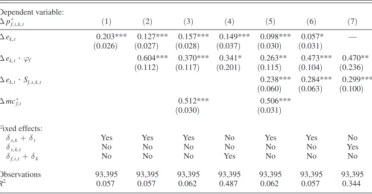
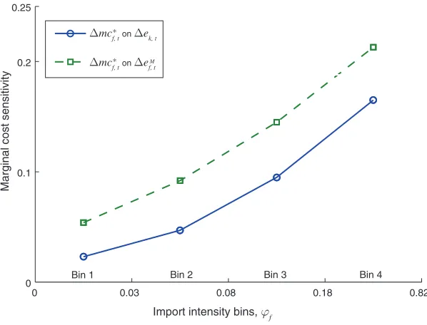
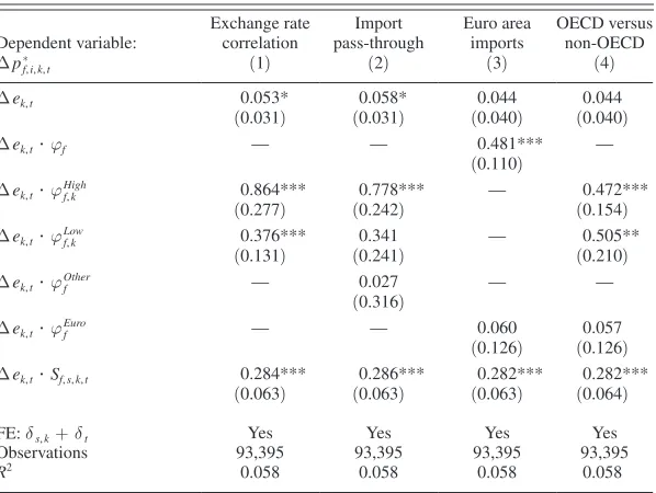
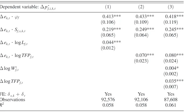
The results provide strong support for the theory. First, we show that import inten-sity is an important correlate of a firm’s exchange rate pass-through, with each addi-tional 10 percentage points of imports in total variable costs reducing pass-through by over 6 percentage points. Second, we show that this effect is due to both the mar-ginal cost channel, which import intensity affects directly, and the markup channel through the selection effect. Finally, when we include market share, which proxies for the markup channel, together with import intensity, we find these two variables jointly to be robust predictors of exchange rate pass-through across different sub-samples and specifications, even after controlling for other firm characteristics such as productivity and employment size.

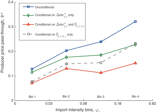
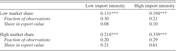
Quantitatively, these results are large. A firm at the fifth percentile of both import intensity and market share (both approximately equal to zero) has a nearly com-plete pass-through ₍94 percent and statistically indistinguishable from 100 percent₎. In contrast, a firm at the ninety-fifth percentile of both import intensity and market share distributions has a pass-through slightly above 50 percent, with import intensity and market share contributing nearly equally to this variation across firms. In other words, while small exporters barely adjust their producer prices and fully pass on the exchange rate movements to foreign consumers, the largest exporters offset almost half of the exchange rate movement by adjusting their prices already at the factory gates. Active markup adjustment by the large firms explains this only in part, and an equally important role is played by the marginal cost channel by means of imported inputs. These results have important implications for aggregate pass-through since the low pass-through firms account for a disproportionately large share of exports.

Related Literature.—Our paper is related to three strands of literature. First, it relates to the recent and growing literature on the interaction of importing and exporting decisions of firms. Earlier work, for example, Bernard, Jensen, and Schott

2 _{Such common forces include the correlations of sector-destination-specific price index, sector-specific} produc-tivity, and cost index with the exchange rate.

(2009₎, has documented a large overlap in the import and export activity of firms.4 Indeed, major exporters are almost always major importers, and this is also true in our dataset. We focus exclusively on the already select group of exporters, most of whom are also importers from multiple source countries. We emphasize the strong selection that still operates within the group of exporters, in particular the hetero-geneity in the intensity with which firms import their intermediate inputs and its consequences for export price pass-through.

Second, our paper is related to the recent empirical and structural work on the relationship between firm import intensity and firm productivity. Although we base our model on Halpern, Koren, and Szeidl (2011), who estimate the effects of imports on total factor productivity for Hungarian firms, similar models were developed in Amiti and Davis (2012) to study the effects of import tariffs on firm wages and in Gopinath and Neiman ₍2014₎ to study the effects of the Argentine trade collapse fol-lowing the currency devaluation of 2001 on the economy-wide productivity.5 _{In our} study, we focus instead on how the interplay between import intensity and markup variability contributes to incomplete exchange rate pass-through.

Third, our paper contributes to the vast literature on the exchange rate disconnect

(see Obstfeld and Rogoff 2001; Engel 2001) and in particular on the incomplete pass-through of exchange rate shocks into international prices. In the past decade, substantial progress has been made in the study of this phenomenon, both theoreti-cally and empiritheoreti-cally.6 _{This literature has explored three channels leading to} incom-plete pass-through. The first channel, as surveyed in Engel (2003), is short-run nominal rigidities with prices sticky in the local currency of the destination market, labeled in the literature as local currency pricing (LCP). Under LCP, the firms that do not adjust prices have zero short-run pass-through. Gopinath and Rigobon ₍2008₎ provide direct evidence on the extent of LCP in US import and export prices. The second channel—pricing-to-market ₍PTM₎—arises in models of variable markups in which firms optimally choose different prices for different destinations depending on local market conditions. Atkeson and Burstein ₍2008₎ provide an example of a recent quantitative investigation of the PTM channel and its implication for inter-national aggregate prices.7 _{Finally, the third channel of incomplete pass-through} into consumer prices often considered in the literature is local distribution costs, as for example in Burstein, Neves, and Rebelo ₍2003₎ and Goldberg and Campa

(2010). Our imported inputs channel is similar in spirit to the local distribution costs in that they make the costs of the firm more stable in the local currency of

4 _{Other related papers include Kugler and Verhoogen (2009); Manova and Zhang (2009); Feng, Li, and Swenson}

(2012); and Damijan, Konings, and Polanec (2012).

5 _{Blaum, Lelarge, and Peters (2013) document stylized facts about import behavior of French firms and provide} another related model. Amiti and Konings (2007) provide an empirical analysis of the micro-level effects of imports on firm productivity.

6 _{For a survey of earlier work, see Goldberg and Knetter (1997), who in particular emphasize that “[l]ess is} known about the relationship between costs and exchange rates” (see p. 1244). The handbook chapter by Burstein and Gopinath (2013) provides a summary of recent developments in this area.

export destination. The difference with the distribution cost channel is that the use of imported inputs results in incomplete pass-through not only into consumer prices, but also into producer factory gate prices.

A related line of literature, surveyed in Goldberg and Hellerstein (2008), has identified the PTM channel by structurally estimating industry demand to back out model-implied markups of the firms. Goldberg and Verboven (2001) apply this methodology in the context of the European car market, while Nakamura and Zerom

(2010) and Goldberg and Hellerstein (2013) study the coffee and the beer markets, respectively, incorporating sticky prices into the analysis. Based on the finding that markups do not vary enough to capture the variation in exporter prices arising from exchange rate volatility, these studies conclude there must be a residual role for the marginal cost channel, due to either the local distribution margin or imported inputs. Our paper is the first to directly estimate the importance of the marginal cost channel for incomplete pass-through into exporter prices arising from the use of imported intermediate inputs.

Our work is closely related to Berman, Martin, and Mayer (2012) in that we also study the variation in pass-through across heterogeneous firms. While they focus on the role of firm productivity and size, we emphasize the role of imported inputs and destination-specific market shares.8 _{Our approach also enables us to provide a} quan-titative decomposition of the contribution of the marginal cost and variable markup channels to incomplete exchange rate pass-through.

The rest of the paper is structured as follows. Section I lays out the theoretical framework and provides the theoretical results that motivate the empirical analysis that follows. Section  II introduces the dataset and describes the stylized patterns of cross-sectional variation in the data. Section  III describes our main empirical findings. Section IV concludes. The technical derivations and additional results are provided in the online Appendix.

I. Theoretical Framework

In this section, we develop a theoretical framework linking a firm’s exchange rate pass-through to its import intensity and export market shares, all of which are endogenously determined. We use this framework to formulate testable implications and to derive an equilibrium relationship, which we later estimate in the data. We start by laying out the two main ingredients of our framework—the Atkeson and Burstein (2008) model of strategic complementarities and variable markups and the Halpern, Koren, and Szeidl ₍2011₎ model of the firm’s choice to import intermedi-ate inputs. We then show how the interaction of these two mechanisms generintermedi-ates new theoretical insights on the determinants of exchange rate pass-through. The key predictions of this theory are that a firm’s import intensity and market shares are positively correlated in the cross section and together constitute a sufficient statistic for the exchange rate pass-through of the firm within sector-export market, with import intensity capturing the marginal cost sensitivity to the exchange rate and market share capturing the markup elasticity.

We characterize the equilibrium relationship among market share, import inten-sity, and pass-through, which holds parametrically independently of the particular general equilibrium environment. The parameter values in this relationship depend on the specifics of the general equilibrium, in particular the equilibrium comove-ment between aggregate variables such as exchange rates, price levels, and cost indexes. Nonetheless, we need not take a stand on the specific general equilibrium assumptions as we directly estimate these parameters using cross-sectional variation between firms within industries and export destinations, without relying on strong partial equilibrium or exchange rate exogeneity assumptions.

To focus our analysis on the relationship between import intensity and pass-through, we make a number of simplifying assumptions. First, we condition our analysis on the subset of exporting firms, and hence we do not model entry, exit, or selection into exporting ₍as, for example, in Melitz 2003₎, but rather focus on the import deci-sions of the firms. Similarly, we do not model the decision to export to multiple des-tinations, but simply take this information as exogenously given. Furthermore, we assume all firms are single-product. In the empirical section we discuss the implica-tions of relaxing these assumpimplica-tions.

Second, we assume flexible price setting as in Atkeson and Burstein (2008) and hence do not need to characterize the currency choice ₍i.e., local versus producer currency pricing). This modeling choice is motivated by the nature of our dataset in which we use unit values as proxies for prices. Empirically, incomplete pass-through is at least in part due to price stickiness in local currency, and in light of this we pro-vide a careful interpretation of our results in Section IIIE.9

Last, while the marginal cost channel emphasized in the paper is inherently a mechanism of real hedging, in modeling firms’ import decisions we abstract from choosing or switching import source countries to better hedge their export exchange rate risk. Empirically, we find that the positive correlation between a firm’s destination-specific exchange rate and its import-weighted exchange rate does not vary with the main firm variables that are the focus of our analysis ₍see Section IIID).10

A. Demand and Markups

Consider a firm producing a differentiated good i in sector s and supplying it to destination market k in period t. Consumers in each market have a nested CES demand over the varieties of goods, as in Atkeson and Burstein (2008). The elasticity

9 _{It is useful to keep in mind that, as shown in Gopinath, Itskhoki, and Rigobon (2010), the flexible-price} pass-through forces shape the currency choice of the firms, i.e., firms with a low pass-through conditional on a price change choose to price in local currency, which further reduces the short-run pass-through of these firms. In this paper, we focus on the endogenous determinants of flexible-price (or long-run) pass-through in the cross section of firms, which in the sticky price environment would also contribute to the prevalence of local currency pricing, with the two forces working in the same direction.

of substitution across the varieties within sectors is _ρ, while the elasticity of substi-tution across sectoral aggregates is η, and we assume ρ > η ≥ 1.

Under these circumstances, a firm i faces the following demand for its product:

(1₎ Q_{k,i = ξ k,i} P −ρ_k,i P _kρ−η D_k ,

where Q_k,i is quantity demanded, _{ξ k,i} is a relative preference ₍quality₎ parameter of the firm, Pk,i is the firm’s price, Pk is the sectoral price index, and Dk is the sectoral demand shifter, which the firm takes as given. Index k emphasizes that all these variables are destination specific. For brevity, we drop the additional subscripts s and t for sector and time, since all of our analysis focuses on variation within a given sector.

The sectoral price index is given by Pk ≡

[

]

∑ i ξ k,i = 1. As a convention, we quote all prices in the local currency of the destina-tion market.

An important characteristic of the firm’s competitive position in a market is its market share given by

(2₎ S_{k,i ≡} _ Pk,i Qk,i ∑ _{i ′} Pk, i ′ Qk, i ′

_{= ξ} k,i

(

Pk,i

_ _P

k

)

where market share is sector-destination-year specific. The effective demand elastic-ity for the firm is then

(3) σ k,i ≡ −

d log Qk,i

_ _{dlog P}

k,i

= ρ(1 − Sk,i) + η Sk,i ,

since _∂ log P_k/∂ log P_{k,i =} S_k,i . In words, the firm faces a demand elasticity that is a weighted average of the within-sector and the across-sector elasticities of substitution with the weight on the latter equal to the market share of the firm. High-market-share firms exert a stronger impact on the sectoral price index, making their demand less sensitive to their own price.

When firms compete in prices, they set a multiplicative markup  k,i

≡ σ k,i/( σ k,i − 1) over their costs. Firms face a demand with elasticity decreasing in the market share, and hence high-market-share firms charge high markups. We now define a measure of the markup elasticity with respect to the price of the firm,

hold-ing constant the sector price index:11

(4) Γ k,i ≡ − ∂

log _{ k,i}

_ _{∂ log P}

k,i

= ___ Sk,i

(

)

(

)

> 0.

A lower price set by the firm leads to an increase in the firm’s market share, making optimal a larger markup. Furthermore, the markup elasticity is also increasing in the market share of the firm: firms with larger markups choose to adjust them by more in response to shocks and to keep their prices and quantities more stable. We sum-marize this discussion in Proposition 1.

PROPOSITION 1: The market share of a firm, S_k,i, is a sufficient statistic for its

markup; both markup  k,i and markup elasticity Γ k,i are increasing in the market

share of the firm.

This theoretical framework has two sharp predictions about the markup. First, the variation in the market share fully characterizes the variation in the markup elasticity across firms. As we discuss in the introduction, this is less than general, and alternative demand structures emphasize other determinants of markup vari-ability. Nonetheless, our empirical analysis shows that this prediction provides a useful approximation across broad sectors and multiple export destinations. Second, markup variability is monotonically increasing in the market share. Although this prediction is also model specific, our empirical analysis provides support for this monotonic relationship ₍see Section IIIC₎.

B. Production and Imported Inputs

We build on Halpern, Koren, and Szeidl ₍2011₎ to model the cost structure of the firm and its choice to import intermediate inputs. Consider a firm i, which uses labor L_i and intermediate inputs X_i to produce its output Y_i according to the production function:

(5) Yi = Ω i X ϕi L i1 −ϕ,

where Ω i is firm productivity. Parameter ϕ ∈ [0, 1] measures the share of intermedi-ate inputs in firm expenditure and is sector specific but common to all firms in the sector.

Intermediate inputs consist of a bundle of intermediate goods indexed by j _{∈ [}0, 1_] and aggregated according to a Cobb-Douglas technology:

(6) Xi = exp

{

∫

γ jlog Xi,j d j

}

The types of intermediate inputs vary in their importance in the production process as measured by _γ j , which satisfy ∫ ₀1 γ j d j = 1. Each type j of intermediate good comes in two varieties—domestic and foreign—which are imperfect substitutes:

(7₎ X_{i,j =}

[

j

1 _ _{1+ζ M}

i,j

ζ _ _1+ζ

]

ζ _,

the domestic and the foreign varieties is ₍1 _{+ ζ) >} 1, and a_j measures the produc-tivity advantage (when aj > 1, and disadvantage otherwise) of the foreign variety. Note that since home and foreign varieties are imperfect substitutes, production is possible without the use of imported inputs. At the same time, imported inputs are useful due both to their potential productivity advantage a_j and to the love-of-variety feature of the production technology (7).

A firm needs to pay a firm-specific sunk cost f_i in terms of labor in order to import each type of the intermediate good. The cost of labor is given by the wage rate W ∗, and the prices of domestic intermediates are _{ V _j∗ _}, both denominated in units of producer currency (hence starred). The prices of foreign intermediates are {  m Uj}, where U_j is the price in foreign currency and _{ m} is the nominal exchange rate mea-sured as a unit of producer currency for one unit of foreign currency.12 _{The total} cost is therefore given by W ∗ L_{i + ∫ 0}1 V ∗_j Z_{i, j} d j _{+ ∫ J}

0,i (  m Uj Mi, j + W ∗ _f

i) d j, where

J0,i denotes the set of intermediates imported by the firm.

With this production structure, we can derive the cost function. In particular, given output Yi and the set of imported intermediates J0,i , the firm chooses inputs to minimize its total costs subject to the production technology in equations ₍5₎–₍7₎. This results in the following total variable cost function net of the fixed costs of importing:

(8) TV C i∗ ( Yi | J0,i) = C

∗

_ B _iϕ _{Ω i} Yi ,

where C ∗ is the cost index for a nonimporting firm.13 _{The use of imported inputs} leads to a cost-reduction factor B_{i ≡} B₍ J_{0,i) =} exp

{

0,i γ j log bj d j

}

bj ≡

[

]

We now describe the optimal choice of the set of imported intermediate goods,

J_0,i. For simplicity, we discuss here the case without uncertainty, and the online Appendix generalizes the results. First, we sort all intermediate goods j by γ j log bj , from highest to lowest. Then, the optimal set of imported intermediate inputs is an interval J0,i = [0, j0,i], with j0,i ∈ [0, 1] denoting the cutoff intermediate good. The optimal choice of j0,i trades off the fixed cost of importing W ∗ fi for the reduction in total variable costs from the access to an additional imported input, which is propor-tional to the total material cost of the firm.14 _{This reflects the standard trade-off that} the fixed cost activity is undertaken provided that the scale of operation (here total spending on intermediate inputs₎ is sufficiently large.

12 _{We denote by m a generic source of imported intermediates, and hence }

m can be thought of as an import-weighted exchange rate faced by the firms. The generalization of the model to multiple import source coun-tries is straightforward; in the data, we measure  m as an import-weighted exchange rate at the firm level, as well as split imports by source country (see Section IIID).

13 _{This cost index is given by C} ∗ _{= ( V} ∗ _{/ϕ )} ϕ _{( W} ∗ _{/(1 − ϕ) )} 1−ϕ _{with V} ∗ _{= exp} { _∫ 0 1 _γ

j log( V j∗ / γ j) d j }. 14 _{The marginal imported input satisfies γ}

j0,ilog bj0,i · TM Ci = W ∗ fi, where the left-hand side is the incremental

benefit proportional to the total material cost of the firm TM C_i ≡ ϕ C ∗ Yi/

[

]

With this cost structure, the fraction of total variable cost spent on imported inter-mediate inputs equals

(9) φ _i = ϕ

∫

0 j0,i

γ j

(

)

where ϕ is the share of material cost in total variable cost and γ j

(

)

Finally, holding the set of imported varieties J0,i constant, this cost structure results in the following marginal cost:

(10₎ M C _i∗ ₌ C ∗ _/[ B _iϕ _{Ω i]}.

The partial elasticity of this marginal cost with respect to the exchange rate

 m equals the expenditure share of the firm on imported intermediate inputs,

φ i = ∂ logM C i∗ /∂ log  m, which emphasizes the role of import intensity in the anal-ysis that follows.

We summarize these results in Proposition 2.

PROPOSITION 2: ₍i₎ Within sectors, firms with larger total material cost or smaller

fixed cost of importing have a larger import intensity, φ _i. (ii) The partial elasticity of the marginal cost of the firm with respect to the ₍import-weighted₎ exchange rate equals φ _i.

C. Equilibrium Relationships

We now combine the ingredients introduced above to derive the optimal price setting of the firm, as well as the equilibrium determinants of the market share and import intensity of the firm. Consider firm i supplying an exogenously given set Ki of destination markets k. The firm sets destination-specific prices by solving

max

Yi ,{ Pk,i, Qk,i } k

{

∑

 k Pk,i Qk,i − C

∗

_ B _iϕ _{Ω i} Yi

}

subject to Y_{i = ∑ k∈ K}

i Qk,i and demand equation (1) in each destination k. We quote

the destination-k price Pk,i in the units of destination-k local currency and use the bilateral nominal exchange rate _{ k} to convert the price to the producer currency, denoting with P k,∗ i ≡  k Pk,i the producer-currency price of the firm for destination k. An increase in _{ k} corresponds to the depreciation of the producer currency. The total cost is quoted in units of producer currency.15 _{Note that we treat the choice} of the set of imported goods J_0,i and the associated fixed costs as sunk by the price setting stage when the uncertainty about exchange rates is realized. The problem

of choosing J_0,i under this circumstance is defined and characterized in the online Appendix and Section IIB provides empirical evidence supporting this assumption.

The firm optimally sets prices in each of its destination markets according to

(11₎ P _k,∗ _{i =} _ σ k,i σ k,i − 1

M C _i∗ , k _∈ K_i ,

where M C i∗ is the marginal cost as defined in (10) and  k,i ≡ σ k,i/( σ k,i − 1) is the multiplicative markup with the effective demand elasticity _{σ k,i} defined in ₍3₎. This set of optimality conditions together with the constraints fully characterizes the allocation of the firm, given industry-level variables. In the online Appendix, we exploit these equilibrium conditions to derive how relative market shares and import intensities are determined in equilibrium across firms, and since these results are very intuitive, here we provide only a brief summary.

We show that other things equal and under mild regularity conditions, a firm with higher productivity Ω i , higher quality/demand ξ k,i , lower fixed cost of importing fi , and serving a larger set of destinations K_i has a larger market share S_k,i and a higher import intensity φ _i . Intuitively, a more productive or high-demand firm has a larger market share and hence operates on a larger scale, which justifies paying the fixed cost for a larger set of imported intermediate inputs, J0,i . This makes the firm more import intensive, enhancing its productivity advantage through the cost-reduction effect of imports (larger Bi in (8)). This implies that, independently of the specifics of the general equilibrium environment, we should expect market shares and import intensities to be positively correlated in the cross section of firms, a pattern that we document in the data in Section II.

D. Imported Inputs, Market Share, and Pass-Through

We are now in a position to relate the firm’s exchange rate pass-through into its export prices with its market share and import intensity. The starting point for this analysis is the optimal price setting equation ₍11₎, which we rewrite as a full log differential:

(12) d log P k,∗ i = dlog  k,i + d logM C i∗ .

Consider first the markup term. Using (2)–(4), we have

(13₎ d log _{ k,i = − Γ k,i(}d log P_{k,i −} d log P_{s,k) +} _ Γ k,i ρ − 1 dlog ξ k,i ,

where converting the export price to local currency yields dlog Pk,i = d log P k,∗ i −

d log _{ k} , and we now make explicit the subscript s to indicate that P_s,k is the industry-destination-specific price index. The markup declines in the relative price of the firm and increases in the firm’s demand shock. From Proposition 1,

Next, the change in the marginal cost in equation ₍10₎ can be decomposed as follows:

(14) dlogM C i∗ = φ id log  m

_

U s

_

_

V s∗

+ d log _ C s∗

_

Ω s

+ ϵ iMC .

This expression generalizes the result of Proposition 2 on the role of import inten-sity φ _i by providing the full decomposition of the change in the log marginal cost. Here U __s and V _ _s∗ are the price indexes for the imported intermediates ₍in foreign currency) and domestic intermediates (in producer currency), respectively. The sub-script s emphasizes that these indexes can be specific to sector s in which firm i oper-ates. Finally, dlog C _ s∗ /

_

Ω s is the log change in the industry-average marginal cost for a firm that does not import any intermediates, and _{ϵ i}MC _{is a firm- idiosyncratic} residual term defined explicitly in the online Appendix and assumed orthogonal to the exchange rate.16

Combining and manipulating equations ₍12₎–₍14₎, we prove our key theoretical result:

PROPOSITION 3: In any general equilibrium, the first-order approximation to the

exchange rate pass-through elasticity into producer-currency export prices of the firm is given by

(15) Ψ k,∗ i ≡ E

{

d log P k,∗ i

_ _{d log }

k

}

where _{( α s,k} , _{β s,k} , _{γ s,k)} are sector-destination specific and depend only on average

moments of equilibrium comovement between aggregate variables common to all firms.

The pass-through elasticity _{Ψ k,}∗ _i measures the equilibrium log change of the destination-k producer-currency price of firm i relative to the log change in the bilat-eral exchange rate, averaged across all possible states of the world and shocks that hit the economy.17 _{Under this definition, the pass-through elasticity is a measure of} equilibrium comovement between the price of the firm and the exchange rate, and not a partial equilibrium response to an exogenous movement in the exchange rate. Thus, we do not need to assume that movements in exchange rates are exogenous, nor do we rely on any source of exogenous variation in our estimation. In fact,

16 _{This orthogonality assumption is necessary for Proposition 3, and it holds provided that firm idiosyncratic} shocks are not systematically correlated with exchange rate movements. More precisely, we allow firm demand, productivity, and import prices to move with exchange rates in arbitrary ways, but we require that the relative demand, productivity, and import prices of any two firms within sector-destination do not systematically change with exchange rate movements.

we allow for arbitrary equilibrium comovement between exchange rates and other aggregate variables, including price and cost indexes.

Proposition 3 shows that we can relate firm-level pass-through to market share and import intensity of the firm, which form a sufficient statistic for cross-sectional variation in pass-through within sector-destination, independently of the specifics of the general equilibrium environment and, in particular, independently of what shocks hit the economy and shape the dynamics of the exchange rate. This relation-ship is the focus of our empirical investigation in the next section. The values of the coefficients in this relationship _{( α s,k}, _{β s,k}, _γ s,k) are sector-destination specific, and, although they depend on the general equilibrium environment in which firms operate, we show in Section IIIA that we can directly estimate them in the data with-out imposing any general equilibrium assumptions.18

Furthermore, the theory provides closed form expressions for the coefficients in

(15). The coefficients α s,k and γ s,k depend on the unconditional moments of equi-librium comovement between the exchange rate and aggregate variables such as the price index in the destination market and the domestic cost index (see the online Appendix₎. For example, pass-through into destination prices is lower ₍i.e., _{α s,k} is higher) in an equilibrium environment where the domestic cost index offsets some of the effects of the exchange rate on marginal costs. And pass-through is relatively lower (i.e., γ s,k is higher) for large market-share firms when the destination price index responds weakly to the exchange rate, because of the stronger strategic com-plementarities in their price setting.

The closed form expression for _{β s,k} highlights the structural determinants of the relationship between pass-through and import intensity:

(16) β s,k = _ 1 1 + _Γ s,k

E

{

· d log (  m

_

U _s/ V _ _s∗ ) __ d log  m

}

where __{Γ s,k} is the markup elasticity evaluated at some average measure of market share S _s,k. Intuitively, β s,k depends on the comovement between export and import exchange rates and the pass-through of import exchange rate into the relative price of imported intermediates, as reflected by the two terms inside the expectation in (16). Indeed, import intensity proxies for the marginal cost correlation with the export exchange rate only to the extent that import and export exchange rates are corre-lated and movements in the import exchange rate are associated with the changes in the import prices of the intermediate inputs. Importantly, we do not restrict the exchange rate pass-through into import prices to be complete. In our empirical work, we directly examine our theoretical mechanism by using the variation in exchange rate correlation and import price pass-through across import source countries.

Proposition 3 predicts that pass-through into destination-currency prices, equal to ₍1 _{− Ψ k,}∗ _{i )}, is lower for more import-intensive firms and for firms with higher

destination market share, provided _{β s,k} and _{γ s,k} are positive.19 _Although theoreti-cally these coefficients can have either sign (or equal to zero), we expect them to be positive, and this is what we find in the data. Intuitively, a more import-intensive firm is effectively hedged from a domestic currency appreciation via decreasing import prices and hence keeps its destination-currency price more stable. Further, a high-market-share firm has a lower pass-through as it chooses to accommodate the marginal cost shocks with a larger markup adjustment as opposed to a larger move-ment in its destination-currency price.

II. Data and Stylized Facts

In this section we describe the dataset that we use for our empirical analysis and the basic stylized facts on exporters and importers.

A. Data Description and Construction of Variables

Our main data source is the National Bank of Belgium, which provided a com-prehensive panel of Belgian trade flows by firm, product (CN 8-digit level), exports by destination, and imports by source country. We merge these data, using a unique firm identifier, with firm-level characteristics from the Belgian Business Registry, comprising information on firms’ inputs, which we use to construct total variable cost measures and total factor productivity estimates. Our sample includes annual data for the period 2000 to 2008, beginning the year after the euro was introduced. We focus on manufacturing exports to the OECD countries outside the euro zone: Australia, Canada, Iceland, Israel, Japan, the Republic of Korea, New Zealand, Norway, Sweden, Switzerland, the United Kingdom, and the United States, account-ing for 58 percent of total non-euro exports.20 _{We also include a robustness test with} the full set of non-euro destinations. We provide a detailed description of all the data sources in the online data Appendix.

The dependent variable in our analysis is the log change in a firm f ’s export price of good i to destination country k at time t, proxied by the change in a firm’s export unit value, defined as the ratio of export values to export quantities:

(17) Δ p ∗ f,i,k,t ≡ Δ log

(

Export valu ef,i,k,t

__ _{Export quantit y}

f,i,k,t

)

where quantities are measured as weights or units. We use the change in the ratio of value to weights, where available, and the change in the ratio of value to units other-wise. We note that unit values are an imprecise proxy for prices because there may

19 _{Note that Proposition 3 provides a linear approximation (15) to the generally nonlinear equilibrium relationship.} In the data, we test directly for the nonlinearity in this relationship and find no statistically significant evidence. Our interpretation is that this is not because nonlinearities are unimportant in general, but because these finer features of the equilibrium relationship are less robust across broad industries that we consider in our analysis. This is why we choose to focus on the first-order qualitative prediction of the theory captured by the approximation in (15).

be more than one distinct product within a CN 8-digit code despite the high degree of disaggregation constituting close to 10,000 distinct manufacturing product cat-egories over the sample period. Some price changes may be due to compositional changes within a product code or due to errors in measuring quantities.21 _{To try to} minimize this problem, we drop all year-to-year unit value changes of plus 200 per-cent or minus 67 perper-cent (around 7 percent of the observations).

A distinctive feature of these data that is critical for our analysis is that they also contain firm-level import values and quantities for each CN 8-digit product code by source country. We include all 234 source countries and all 13,000 product codes in the sample. Studies that draw on price data have not been able to match import and export prices at the firm level. In general, many firms engaged in exporting also import their intermediate inputs. In Belgium, around 80 percent of manufacturing exporters import some of their inputs. We use these data to construct three key vari-ables—the import intensity from outside the euro zone φ f,t , the log change in the marginal cost _Δ m c _f,∗ _t , and the firm’s market share S_f,s,k,t . Specifically,

(18_{) φ} f,t ≡

Total non-euro import valu e_f,t

___ _{Total variable cost s}

f,t

,

where total variable costs comprise a firm’s total wage bill and total material cost. We often average this measure over time to obtain a firm-level average import inten-sity denoted by φ f .

The change in marginal cost is defined as the log change in unit values of firm imports from all source countries weighted by respective expenditure shares:

(19_{) Δ} m c _f,∗ _{t ≡}

∑

j_∈ Jf,t

∑

m_∈ Mf,t

ω f,j,m,t Δ log U f,∗ j,m,t ,

where U f,∗ j,m,t is the euro price (unit value) of firm f ’s imports of intermediate good j from country m at time t, the weights _{ω f,j,m,t} are the average of period t and t ₋ 1 shares of respective import values in the firm’s total variable costs, and Jf,t and Mf,t denote the set of all imported goods and import source countries ₍including inside the euro zone) for the firm at a given time. Note that this measure of the marginal cost is still a proxy since it does not reflect the costs of domestic inputs and firm productivity. We control separately for estimated firm productivity and average firm wage rate, however, detailed data on the prices and values of domestic inputs are not available. Nonetheless, controlling for our measure of the firm-level marginal cost is a substantial improvement over previous pass-through studies that typically control only for the aggregate manufacturing wage rate or producer price level.

Furthermore, our measure of marginal cost arguably captures the component of the marginal cost most sensitive to exchange rate movements.

Ideally, we would like to construct _φ f,t and Δ m c f,∗ t for each of the products i a firm produces; however, this measure is available only at the firm-f level, which may not be the same for all of the products produced by multiproduct firms. To address this multiproduct issue, we keep only the firm’s main export products, which we identify using Belgium’s input-output table for the year 2005, comprising 56 IO manufactur-ing codes. For each firm, we identify an IO code that accounts for its largest export value over the whole sample period and keep only the CN 8-digit products within this major-IO code. The objective is to keep only the set of products for each firm that have similar production technologies. This leaves us with 60  percent of the observations but 90 percent of the value of exports. We also present results with the full set of export products and experiment with defining the major product using more disaggregated product lines, such as HS 4-digit.22 _{Further, it is possible that} some of the firm’s imports might be final goods rather than intermediate inputs. We attempt to identify imported intermediate inputs using a number of different approaches. First, we omit any import from the construction of _φ f,t that is defined as a final product using Broad Economic Codes (BEC). Second, we construct φ f using only the intermediate inputs for a given industry according to the IO tables.

The last key variable in our analysis is a firm’s market share, which we construct as follows:

(20) Sf,s,k,t ≡

Export valu ef,s,k,t

__ ∑ _{f ′∈ Fs,k,t} Export valu e _{f ′,s,k,t} ,

where s is the sector in which firm f sells product i and F_s,k,t is the set of Belgian firms that export to destination k, in sector s at time t. Therefore, Sf,s,k,t measures a Belgium firm’s market share in sector s, export destination k at time t relative to all other Belgium exporters. Note that, following the theory, this measure is des-tination specific. The theory also suggests that the relevant measure is the firm’s market share relative to all firms supplying the destination market in a given sector, including exporters from other countries as well as domestic competitors in mar-ket k. But, since our analysis is across Belgian exporters within sector-destinations, the competitive stance in a particular sector-destination is common for all Belgian exporters, and hence our measure of Sf,s,k,t captures all relevant variation for our analysis ₍see Section IIIA₎.23 _{We define sectors at the HS 4-digit level, at which we}

22 _{By only keeping the firm’s major products, we also deal with the potential problem of including products that} firms export but do not produce—a phenomenon referred to as carry-along trade (Bernard et al. 2012). As a further robustness check, in Section IIIE we use IO tables to isolate the inputs that are used in the production of firms’ major products, and only use these inputs to construct the firm’s import intensity variable. See De Loecker et al.

(2012) for an alternative structural treatment of multiproduct firms.

both obtain a nontrivial distribution of market shares and avoid having too many sector-destinations served by a single firm.24

B. Stylized Facts About Exporters and Importers

A salient pattern in our dataset is that most exporters are also importers, a pat-tern also present in many earlier studies cited in the introduction. As reported in Table  1, in the full sample of Belgian manufacturing firms, the fraction of firms that are either exporters or importers is 33 percent. Out of these firms, 57 percent both import and export, 27 percent only import, and 16 percent only export. That is, 24 percent of manufacturing firms in Belgium export and 78 percent of exporters also import.25 _{This high correlation between exporting and importing suggests that} the selection into both activities is driven by the same firm characteristics, such as productivity, which determines the scale of operations. We show how this overlap in importing and exporting activities turns out to be important for understanding the incomplete exchange rate pass-through.

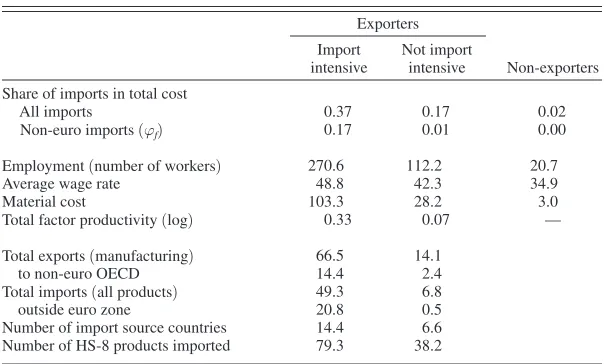
Interestingly, the data reveal a lot of heterogeneity within exporting firms, which are an already very select subsample of firms. The large differences between export-ers and nonexportexport-ers are already well-known and are also prevalent in our data. The new stylized facts we highlight here are the large differences within exporters between high- and low-import-intensity exporting firms. We show in Table 2 that these two groups of exporting firms differ in fundamental ways. We report various firm-level characteristics for high- and low-import-intensity exporters, splitting exporters into two groups based on the median import intensity outside the euro zone _{( φ} f ) equal to 4.2 percent.26 For comparison, we also report the available analo-gous statistics for nonexporting firms with at least five employees.

24 _{The median of S}

f,s,k,t is 7.8 percent, yet the seventy-fifth percentile is over 40 percent and the export-value-weighted median is 55 percent. Twenty-four percent of Sf,s,k,t observations are less than 1 percent, yet these observations account for only 1.4 percent of export sales. Three percent of Sf,s,k,t observations are unity, yet they account for less than 2.5  percent. Our results are robust (and, in fact, become marginally stronger) to the exclusion of observations with very small and very large market shares. We depict the cumulative distribution function of Sf,s,k,t in Figure A1 in the online Appendix.

25 _{These statistics are averaged over the sample length, but they are very stable year-to-year. In the subsample of} exporters we use for our regression analysis in Section IIIB, the fraction of importing firms is somewhat higher at 85.5 percent, reflecting the fact that data availability is slightly biased toward larger firms.

26 _{The unit of observation here is a firm-year. If we split our sample based on firm-product-destination-year}

(which is the unit of observation in our regression analysis), the median import intensity is higher at 8.2 percent, however, this has no material consequences for the patterns we document in Table 2.

Table 1—Exporter and Importer Incidence ( percent)

Exporters and/or importers All exporters

Fraction of all firms 32.6 23.7

Among them

exporters and importers 57.0 78.4

only exporters 15.8 21.6

only importers 27.2 —

From Table  2, we see that import-intensive exporters operate on a larger scale and are more productive. The share of imported inputs in total variable costs for import-intensive exporters is 37  percent compared to 17  percent for nonimport-intensive exporters, and similarly for imports sourced outside the euro zone it is 17 percent compared to 1.2 percent. And of course, these numbers are much lower for nonexporters at 1.6 percent for imports outside Belgium and 0.3 percent for imports outside the euro zone. Import-intensive exporters are 2.5 times larger in employment than nonimport-intensive exporters and 13 times larger than nonex-porters; they pay a 15 percent wage premium relative to nonimport-intensive firms and a 40 percent wage premium relative to nonexporters. Similarly, import-intensive exporters have much larger total material costs, total factor productivity, and market share. These firms also export and import on a much larger scale, and are more likely to trade with more distant countries outside the euro zone. These firms import more in terms of total value, number of imported goods, and from a larger set of import source countries. These results highlight that both types of exporting firms are active in importing from a range of countries both within and outside the euro zone but that the two types of firms differ substantially in import intensity, consistent with the predictions of our theoretical framework.

We now provide more details on the distribution of import intensity outside the euro zone _{( φ} f). We see that the distribution of import intensity among exporters in Table 3, although somewhat skewed toward zero, has a wide support and sub-stantial variation, which we exploit in our regression analysis in Section III. Over 24 percent of exporters do not import from outside the euro zone, yet they account for only 1 percent of Belgian manufacturing exports. For the majority of firms, the

Table 2—Import-Intensive Exporters

Exporters Import intensive

Not import

intensive Non-exporters

Share of imports in total cost

All imports 0.37 0.17 0.02

Non-euro imports _{( φ f)} 0.17 0.01 0.00

Employment ₍number of workers₎ 270.6 112.2 20.7

Average wage rate 48.8 42.3 34.9

Material cost 103.3 28.2 3.0

Total factor productivity (log) 0.33 0.07 —

Total exports (manufacturing) 66.5 14.1

to non-euro OECD 14.4 2.4

Total imports (all products) 49.3 6.8

outside euro zone 20.8 0.5

Number of import source countries 14.4 6.6

Number of HS-8 products imported 79.3 38.2

share of imported inputs in total costs ranges between 0 and 10 percent, while the export-value-weighted median of import intensity is 13 percent. At the same time, nearly 28 percent of export sales are generated by the firms with import intensity in excess of 30  percent.27 _{We further depict the cumulative distribution function} of import intensity φ f in Figure A1 in the online Appendix, which also provides a cumulative distribution function for our market share variable S_f,s,k,t .

Table 4 displays the correlations of import intensity with other firm-level variables in the cross section of firms. Confirming the predictions of Section IC, import inten-sity is positively correlated with market share, as well as with firm TFP, employment, and revenues. The strongest correlate of import intensity is the total material cost of the firm, consistent with the predictions of Proposition 2. Overall, the correlations in Table 4 broadly support the various predictions of our theoretical framework. At the same time, although import intensity and market share are positively correlated with productivity and other firm performance measures, there is sufficient indepen-dent variation to enable us to distinguish between the determinants of incomplete pass-through in the following subsections.

27 _{While the unweighted distribution (firm count) has a single peak, the export-value-weighted distribution has} two peaks. This is due to the fact that one exporter with φ f = 0.33 accounts for almost 14 percent of export sales. Our results are not sensitive to the exclusion of this largest exporter, which accounts for only 134 observations out of a total of over 90,000 firm-destination-product-year observations in our sample.

Table 3—Distribution of Import Intensity among Exporters

Number of firms

Fraction of firms

(percent) Fraction of export value(percent)

φf =0 717 24.9 1.4

0 _{< φ f ≤} 0.1 1,478 51.3 38.2

0.1 < φ f ≤ 0.2 348 12.1 23.8

0.2 _{< φ f ≤} 0.3 155 5.4 8.8

0.3 < φ f ≤ 0.4 94 3.3 23.0

φ f > 0.4 89 3.1 4.9

Note: Import intensity, φf , is the share of imported intermediate inputs from outside the euro

zone in the total variable cost of the firm, averaged over the sample period.

Table 4—Correlation Structure of Import Intensity

Import

intensity TFP Revenues Employment

Material cost

Market share 0.16 0.20 0.28 0.25 0.27

Material cost 0.23 0.70 0.99 0.83

Employment 0.10 0.60 0.86

Revenues 0.21 0.72

TFP 0.15

We close this section with a brief discussion of the patterns of time-series varia-tion in import intensity for a given firm. Import intensity appears to be a relatively stable characteristic of the firm, moving little over time and in response to exchange rate fluctuations. Specifically, the simple regression of φ f,t on firm fixed effects has an R2 _{of over 85 percent, implying that the cross-sectional variation in time-averaged} firm import intensity φ f is nearly six times larger than the average time-series varia-tion in _φ f,t for a given firm. When we regress the change in φ f,t on firm fixed effects and the lags of the log change in firm-level import-weighted exchange rates, the contemporaneous effect is significant with a semi-elasticity of only 0.057, and with offsetting, albeit marginally significant, lag effects. That is, a 10 percent deprecia-tion of the euro temporarily increases import intensity by 0.57 of a percentage point. Furthermore, we find that the firm hardly adjusts its imports on the extensive margin in response to changes in its import-weighted exchange rate.28 _{All of this evidence} provides support for our assumption in Section I that the set of imported goods is a sunk decision at the horizons we consider, and hence the extensive margin plays a very limited role in the response of a firm’s marginal cost to exchange rate move-ments, justifying the use of _φ f as a time-invariant firm characteristic in the empirical regressions that follow.

To summarize, we find substantial variation in import intensity among export-ers, and this heterogeneity follows patterns consistent with the predictions of our theoretical framework. Next, guided by the theoretical predictions, we explore the implications of this heterogeneity for the exchange rate pass-through patterns across Belgian firms.

III. Empirical Evidence

This section presents our main empirical results. We start by introducing and estimating our main empirical specification. We then provide nonparametric evi-dence and explore the forces behind our empirical results, confirming the specific mechanisms identified by the theory. We conclude with a battery of robustness tests.

A. Empirical Specification

We now turn to the empirical estimation of the relationship between import intensity, market share, and pass-through in the cross section of exporters

(Proposition 3). The theoretical pass-through regression equation (15) cannot be directly estimated since pass-through _{Ψ k,}∗ _i is not a variable that can be observed in the data. Therefore, we step back to the decomposition of the log price change in equations ₍12₎–₍14₎, which we again linearize in import intensity and market share. After replacing differentials with changes over time Δ, we arrive at our main empirical specification, where we regress the annual change in log export

price on the change in the log exchange rate, interacted with import intensity and market share:

(21) Δ p f,∗ i,k,t   = [ α s,k + β φ f,t−1 + ˜ γ Sf,s,k,t₋1]Δ ek,t

+ δ s,k + b φ f,t−1 + c Sf,s,k,t₋1 + ˜ u f,i,k,t ,

where p f,∗ i,k,t is the log euro producer price to destination k (as opposed to local-currency price₎, and an increase in the log nominal exchange rate, e_k,t, cor-responds to the bilateral depreciation of the euro relative to the destination-k cur-rency.29 _{In our analysis we estimate parameters β and ˜ γ with values averaged across} sector-destination-years. In order to keep the pool of averaged coefficients ( β s,k , γ s,k) relatively homogenous, we focus on manufacturing exports to high-income OECD countries in our benchmark specifications. The regression equation (21) is a struc-tural relationship that emerges from the theoretical model of Section I, and S_f,s,k,t−1 corresponds to our measure of market share defined in equation (20). Under a mild assumption that _Δ e_k,t is uncorrelated with _{( φ} f,t₋1 , Sf,s,k,t−1), we prove the following proposition in the online Appendix:

PROPOSITION 4: The OLS estimates of β and ˜ γ in (21) identify the weighted averages across sector-destination-years of _{β s,k} and _γ s,k S s,k,t−1 respectively,

where S s,k,t₋1 is the sector-destination-time-specific cumulative market share of all

Belgian exporters and _{( β s,k} , _{γ s,k)} are the theoretical coefficients in the pass-through relationship (15).

This result shows that, despite the fact that we cannot directly estimate the theo-retical regression ₍15₎, we can nonetheless identify the theoretical coefficients in the relationship between pass-through, import intensity, and market share. Furthermore, it formally confirms the validity of our measure of the market share relative to other Belgian exporters.

Equation ₍21₎ is our benchmark empirical specification. Note that it is very demanding in that it requires including sector-destination dummies and their inter-actions with exchange rate changes at a very disaggregated level. Therefore, we start by estimating equation (21) with a common coefficient α, and later replace sector-destination fixed effects _{δ s,k} with sector-destination-year fixed effects _{δ s,k,t} which absorb α s,k Δ ek,t .We also estimate (21) for exports to a single destination

(United States₎ only. In our main regressions we replace _φ f,t₋1 with a time-invariant

φ f to reduce the measurement error, and also to maximize the size of the sample since some of the lagged _φ f,t₋1 were unavailable. This has little effect on the results since, as we show, φ f,t is very persistent over time. In the main specifications we also replace S_f,s,k,t−1 with the contemporaneous S_f,s,k,t , as both give the same results.30 _In the robustness section we report the estimates from the specification with the lagged

φ f,t₋1 and Sf,s,k,t−1 .

29 _{The nominal exchange rates are average annual rates from the IMF. These are provided for each country} rela-tive to the US dollar, which we convert to be relarela-tive to the euro.