The Degrees of Freedom Region of
Temporally-Correlated MIMO Networks
with Delayed CSIT
Xinping Yi,
Student Member, IEEE, Sheng Yang,
Member, IEEE,
David Gesbert,
Fellow, IEEE, Mari Kobayashi,
Member, IEEE
Abstract—We consider the temporally-correlated Multiple-Input Multiple-Output (MIMO) broadcast channels (BC) and interference channels (IC) where the transmitter(s) has/have (i) delayed channel state information (CSI) obtained from a latency-prone feedback channel as well as (ii) imperfect current
CSIT, obtained, e.g., from prediction on the basis of these past channel samples based on the temporal correlation. The degrees of freedom (DoF) regions for the two-user broadcast and interference MIMO networks with general antenna configuration under such conditions are fully characterized, as a function of the prediction quality indicator. Specifically, a simple unified framework is proposed, allowing to attain optimal DoF region for the general antenna configurations and current CSIT qualities. Such a framework builds upon block-Markov encoding with
interference quantization, optimally combining the use of both outdated and instantaneous CSIT. A striking feature of our work is that, by varying the power allocation, everypoint in the DoF region can be achieved with one single scheme. As a result, instead of checking the achievability of every corner point of the outer bound region, as typically done in the literature, we propose a new systematic way to prove the achievability.
Index Terms—MIMO, Broadcast Channels, Interference Chan-nels, Degrees of Freedom, Delayed CSIT
I. INTRODUCTION
While the capacity region of the Input Multiple-Output (MIMO) broadcast channel (BC) was established in [1], the characterization of the capacity of Gaussian interference channel (IC) has been a long-standing open problem, even for the two-user single-antenna case. Recent progress sheds light on this problem from various perspectives, among which the authors in [2] characterized the degrees of freedom (DoF) region, specializing to the large signal-to-noise-ratio (SNR) regime, for the two-user MIMO IC. The number of DoF represents the slope with which the rate increases with the logarithm of SNR. Note that when taking additional system limitations into account such as imperfect hardware, finite
Manuscript received October 10, 2012; revised June 05, 2013; accepted September 30, 2013. This work has been performed in the framework of the European research projects HARP, SHARING and HIATUS (FET-Open grant number: 265578), as well as the French ANR project FIREFLIES (ANR-10-INTB-0302). A part of preliminary results of this work has been presented at IEEE Int. Symp. Inf. Theory 2013, Istanbul, Turkey.
X. Yi and D. Gesbert are with the Mobile Communications Dept., EURECOM, 06560 Sophia Antipolis, France (email: {xinping.yi, david.gesbert}@eurecom.fr).
S. Yang and M. Kobayashi are with the Telecommunications Dept., SUPELEC, 91190 Gif-sur-Yvette, France (e-mail: {sheng.yang, mari.kobayashi}@supelec.fr).
modulation levels, and cost of channel training in a time-varying environment, the sum rate inevitably saturates in the very large SNR limit [3]. However, the DoF can be shown to be meaningful within a reasonable interval of practical SNRs for properly designed systems. Furthermore, it provides us with a first-order approximation from which novel transmission schemes and insights emerge. In most works, the DoF analysis for multiuser channels involves the full knowledge of channel state information (CSI) at both the transmitter and receiver sides. In practice, however, the acquisition of perfect CSI at the transmitters is difficult, if not impossible, especially for fast fading channels. The CSIT obtained via feedback suffers from delays, which renders the available CSIT feedback possibly fully obsolete (i.e., uncorrelated with the current true channel) under the fast fading channel and, seemingly non-exploitable in view of designing the spatial precoding.
Recently, this common accepted viewpoint in such scenario (referred to as “delayed CSIT”) was challenged by an interest-ing information theoretic work [4], in which a novel scheme (termed here as “MAT alignment”) was proposed for the MISO BC to demonstrate that even the completely outdated channel feedback is still useful. The precoders are designed achieving strictly better DoF than what is obtained without any CSIT. The essential ingredient for the proposed scheme in [4] lies in the use of a multi-slot protocol initiating with the transmission of unprecoded information symbols to the user terminals, followed by the analogforwarding of the interferences created in the previous time slots. Most recently, generalizations under the similar principle to the MIMO BC [5], MIMO IC [6] settings, the MIMO BC with secrecy constraints [7], among others, were also addressed, where the DoF regions are fully characterized with arbitrary antenna configurations, again establishing DoF strictly beyond the ones obtained without CSIT [8]–[10] but below the ones with perfect CSIT [1], [2]. Note that other recent interesting lines of work combining instantaneous and delayed forms of feedback were reported in [11], [12].
information about the current one. Therefore a scenario where the transmitter is endowed with delayed CSI in addition to some (albeit imperfect) estimate of the current channel is of practical relevance. Together with the delayed CSIT, the benefit of such imperfect current CSIT was first exploited in [13] for the MISO BC whereby a novel transmission scheme was proposed which improves over pure MAT alignment in constructing precoders based on delayed and current CSIT estimate. The full characterization of the optimal DoF for this hybrid CSIT was later reported in [14], [15] for MISO BC under this setting. The key idea behind the schemes (termed hereafter as “α-MAT alignment”) in [13]–[15] lies in the modification of the MAT alignment such that i) the initial time slot involves transmission of precodedsymbols, which enables to reduce the power of mutual interferences and efficiently compress them; ii) the subsequent slots perform a digital transmission of quantized residual interferences together with new private symbols. Most recently, this philosophy was extended to the MIMO networks (BC/IC) but only with symmetric antenna configurations [16], as well as the K-user MISO case [17]. The generalization to the MISO BC with different qualities of imperfect current CSIT was also studied in [18]. Remarkably, the authors of [18] showed that, in order to balance the asymmetry of the CSIT quality, an infinite number of time slots are required. As such, they extended the number of phases of the α-MAT alignment [14] to infinity and varied the length of each phase. Unfortunately, extending the previous results to the MIMO case with arbitrary antenna configurations is not a trivial step, even with the symmetric current CSIT quality assumption. The main challenges are two-fold: (a) the extra spatial dimension at the receiver side introduces a non-trivial tradeoff between the useful signal and the mutual interference, and (b) the asymmetry of receive antenna configurations results in the discrepancy of common-message-decoding capability at different receivers. In particular, the total number of streams that can be delivered as common messages to both receivers is inevitably limited by the weaker one (i.e., with fewer antennas). Such a constraint prevents the system from achieving the optimal DoF of the symmetric case by simply extending the previous schemes developed in [16].
To counter these new challenges posed by the asymmetry of antenna configurations, we develop a new strategy that balances the discrepancy of common-message-decoding capability at two receivers. This allows us to fully characterize the DoF region of both MIMO BC and MIMO IC, achieved by a unified and simple scheme built upon block-Markov encoding. This encoding concept was first introduced in [19] for relay channels and then became a standard tool for communication problems involving interaction between nodes, such as feedback (e.g., [20], [21]) or user cooperation (e.g., [22]). It turns out that our problem with both delayed and instantaneous CSIT, closely related to [20], can also be solved with this scheme. As it will become clear later, in each block, the transmitter superimposes the common information about the interferences created in the past block (due to the imperfect instantaneous CSIT) on the new private information (thus creating new interferences). At the receiver side, backward decoding is employed, i.e., the decoding of each block relies on the common side information from the
decoding of future blocks. Due to the repetitive nature in each block, the proposed scheme can be uniquely characterized with the parameters such as the power allocation and rate splitting of the superposition. Surprisingly enough, our block-Markov scheme can also include the asymmetry of current CSIT with a simple parameter change, and thus somehow balance the global asymmetry, i.e., antenna asymmetry and CSIT asymmetry, in the system.
Overall, our results allow to bridge between previously reported CSIT scenarios such as the pure delayed CSIT of [4], [5] and the pure instantaneous CSIT scenarios [1], [2] for the MIMO setting. We tackle both the BC and IC configurations as we point out the tight connection between the DoF achieving transmission strategies in both settings. More specifically, we obtain the following key results:
• We establish outer bounds on the DoF region for the two-user temporally-correlated MIMO BC and IC with perfect delayed and imperfect current CSIT, as a function of the current CSIT quality exponent. By introducing a virtual received signal for the IC, we nicely link the outer bound to that of the BC, arriving at the similar outer bound results for both cases. In addition to the genie-aided bounding techniques and the application of the extremal inequality in [14], we develop a set of upper and lower bounds of ergodic capacity for MIMO channels, which is essential for the MIMO case but not extendible from MISO. • We propose a unified framework relying on block-Markov
encoding uniquely parameterized by the rate splitting and power allocation, by which the optimal DoF regions confined by the outer bounds are achievable with perfect delayed plus imperfect current CSIT. For any antenna and current CSIT settings, every point in the outer bound region can be achieved with one single scheme. For instance, the MIMO BC with M = 3, N1 = 2 and
N2 = 1 achieves optimal sum DoF 15+4α71+2α2 when
3α1−2α2 ≤ 1 and 7+23α2 otherwise, where α1 and
α2 are imperfect current CSIT qualities for both users’
channels. This smoothly connects three special cases: the case with pure delayed CSIT [5] (α1 = α2 = 0), that
with perfect current CSIT [1] (α1=α2= 1), and that
with perfect CSIT at Receiver 1 and delayed CSIT at Receiver 2 [24] (α1= 1, α2= 0).
• We propose a new systematic way to prove the achievabil-ity. In the proposed framework, the achievability region is defined by the decodability conditions in terms of the rate splitting and power allocation. The achievability is proved by mapping the outer bound region into a set of proper rate and power allocation and showing that this set lies within the decodability region. This contrasts with most existing proofs in the literature where the achievability of each corner point is checked.
special MISO case [13]–[15] with N1=N2= 1, symmetric
MIMO case [16], as well as the MISO case with asymmetric current CSIT qualities [18]. In a parallel work [23], a similar scheme was independently revealed, also built on the block-Markov encoding, evolving from the multi-phase scheme initially proposed in [18]. While they focus on the MISO BC in a more general evolving CSIT setting, our work deals with a wider class of channel configurations (both MIMO BC and IC) with static CSIT.
The rest of the paper is organized as follows. We present the system model and assumptions in the coming section, followed by the main results on DoF region characterization for both MIMO BC and MIMO IC cases in Section III. Some illustrative examples of the achievability schemes are provided in Section IV, followed by the general formulation in Section V. In Section VI, we present the proofs of outer bounds. Finally, we conclude the paper in Section VII.
Notation: Matrices and vectors are represented as uppercase and lowercase letters, respectively. Matrix transport, Hermitian transport, inverse, rank, determinant and the Frobenius norm of a matrix are denoted byAT,AH,A−1,rank(A),det(A)and kAkF, respectively.A[k1:k2]represents the submatrix ofAfrom
k1-th row tok2-th row whenk1≤k2.h⊥ is the normalized
orthogonal component of any non-zero vectorh. We useIM
to denote an M ×M identity matrix where the dimension is omitted whenever confusion is not probable. The approximation
f(P)∼ g(P) is in the sense oflimP→∞gf((PP)) =C, where
C >0 is a constant that does not scale asP. Partial ordering of Hermitian matrices is denoted by and, i.e., AB
meansB−Ais positive semidefinite. Logarithms are in base 2.
(x)+ meansmax{x,0}, and
Rn+ represents the set ofn-tuples
of non-negative real numbers.f =O(g)follows the standard Landau notation, i.e., limfg ≤C where the limit depends on the context. With some abuse of notation, we use OX(g)to
denote anyf such thatEX(f) =O(EX(g)). Finally, the range
or null spaces mentioned in this paper refer to the column spaces.
II. SYSTEMMODEL
A. Two-user MIMO Broadcast Channel
For a two-user (M, N1, N2) MIMO broadcast channel
(BC) with M antennas at the transmitter and Ni antennas at Receiveri, the discrete time signal model is given by
yi(t) =Hi(t)x(t) +zi(t) (1)
for any time instantt, whereHi(t)∈CNi×M is the channel
matrix for Receiver i (i = 1,2); zi(t) ∼ NC(0,INi) is the
normalized additive white Gaussian noise (AWGN) vector at Receiver i and is independent of channel matrices and transmitted signals; the coded input signal x(t)∈ CM×1 is subject to the power constraint E kx(t)k2≤P,∀t.
B. Two-user MIMO Interference Channel
For a two-user (M1, M2, N1, N2)MIMO interference
chan-nel (IC) withMi antennas at Transmitter iandNj antennas
at Receiverj, for i, j= 1,2, the discrete time signal model is given by
yi(t) =Hi1(t)x1(t) +Hi2(t)x2(t) +zi(t) (2)
for any time instantt, whereHji(t)∈CNj×Mi (i, j = 1,2)
is the channel matrix between Transmitter iand Receiver j; the coded input signalxi(t)∈CMi×1 is subject to the power
constraintE kxi(t)k2≤P for i= 1,2,∀t.
In the rest of this paper, we refer to MIMO BC/IC as MIMO networks. For notational brevity, we define the ensemble of channel matrices, i.e.,H(t),{H1(t),H2(t)} (resp.H(t), {H11(t),H21(t),H12(t),H22(t)}), as the channel state for
BC (resp. IC). We further defineHk
,{H(t)}k
t=1, andHˆk , {Hˆ(t)}k
t=1, where k= 1,· · ·, n.
C. Assumptions and Definitions
Assumption 1 (perfect delayed and imperfect current CSIT). At each time instant t, the transmitters know perfectly the delayed CSI Ht−1, and obtain an imperfect estimate of the
current CSIHˆ(t), which could, for instance, be produced by standard prediction based on past samples. The current CSIT estimate is modeled by
Hi(t) = ˆHi(t) + ˜Hi(t) (3)
Hij(t) = ˆHij(t) + ˜Hij(t) (4)
for BC and IC, respectively, where estimation error H˜i(t)
(resp.H˜ij(t)) and the estimateHˆi(t)(resp.Hˆij(t)) are
mutu-ally independent, and each entry is assumed1to beN C 0, σ
2
i
andNC 0,1−σ2i. Further, we assume the following Markov chain
(Ht−1,Hˆt−1)→Hˆ(t)→ H(t), ∀t,
(5)
which meansH(t)is independent of(Ht−1,Hˆt−1)conditional
onHˆ(t). Furthermore, at the end of the transmission, i.e., at time instantn, the receivers know perfectlyHn and Hˆn.
It readily follows that, for any fat submatrixHofHiorHij,
E(log det(HHH)) > −∞ and E(log det( ˆHHˆH)) = O(1) when σ2
i goes to 0.
The assumption on the CSI at the receiver (CSIR) is in accordance with previous works with delayed CSIT, and does not add any limitation over the assumption made in [4]–[6]. We point out that only local CSIT/CSIR (the channel links with which the node is connected) is really helpful and leads to the same result. Nevertheless, we assume the CSIT/CSIR to be available in a global fashion for simplicity of presentation. We are interested in characterizing the degrees of freedom (DoF) of the above system as functions of the quality of current CSIT, thus bridging between the two previously investigated extremes which are the perfect instantaneous CSIT and the fully outdated (non-instantaneous) CSIT cases. As it was established in previous works [13], [14], the imperfect current CSIT has beneficial value (in terms of improving the DoF) only if the CSIT estimation error decays at least exponentially with the
1We make the above assumption on the fading distribution to simplify
d1≤min{M, N1}, (6a)
d2≤min{M, N2}, (6b)
d1+d2≤min{M, N1+N2}, (6c)
d1
min{M, N1}
+ d2
min{M, N1+N2}
≤1 +min{M, N1+N2} −min{M, N1} min{M, N1+N2}
α1, (6d)
d1
min{M, N1+N2}
+ d2 min{M, N2}
≤1 +min{M, N1+N2} −min{M, N2} min{M, N1+N2}
α2, (6e)
SNR or faster. Thus it is reasonable to study the regime by which the CSIT quality can be parameterized by an indicator
αi≥0 such that:
αi,− lim P→∞
logσ2
i
logP (7)
if the limit exists. Thisαiindicates the quality of current CSIT corresponding to Receiveriat high SNR. Whileαi= 0reflects the case with no current CSIT, αi→ ∞ corresponds to that with perfect instantaneous CSIT. As a matter of fact, when
αi≥1, the quality of the imperfect current CSIT is sufficient to avoid the DoF loss, and ZF precoding with this imperfect CSIT is able to achieve the maximum DoF [27]. Therefore, we focus on the caseαi∈[0,1]henceforth. The connections
between the above model and the linear prediction over existing time-correlated channel models with prescribed user mobility are highlighted in [13], [14]. According to the definition of the estimated current CSIT, we have E |hH
k(t)ˆh⊥k(t)|2
=σ2
i ∼ P−αi, withhH
krepresenting any row of channel matricesHi(t)
(resp.Hij(t)), andhˆHk being its corresponding estimate.
A rate pair(R1, R2)is said to beachievablefor the two-user
MIMO networks with perfect delayed and imperfect current CSIT if there exists a 2nR1,2nR2, ncode scheme with:
• two message sets W1,[1 : 2nR1]andW2,[1 : 2nR2],
from which two independent messages W1 and W2
intended respectively to Receiver 1 and Receiver 2 are uniformly chosen;
• one encoding function for (each) transmitter:
BC: x(t) =ft W1, W2,Ht−1,Hˆt
IC: xi(t) =fi,t Wi,Ht−1,Hˆt
, i= 1,2; (8)
• one decoding function at the corresponding receiver,
ˆ
Wj =gj Yjn,H n, ˆ
Hn
, j= 1,2 (9)
for Receiver j, where Yn
j ,{yj(t)}nt=1,
such that the average decoding error probability Pe(n), defined
as Pe(n) ,P (W1, W2) 6= ( ˆW1,Wˆ2)
, vanishes as the code length n tends to infinity. The capacity region C is defined as the set of all achievable rate pairs. Accordingly, the DoF region can be defined as follows:
Definition 1 (degrees of freedom region). The degrees of freedom (DoF) region for the two-user MIMO network is defined as
D=
(d1, d2)∈R2+| ∀(w1, w2)∈R2+, w1d1+w2d2
≤lim sup P→∞
sup
(R1,R2)∈C
w1R1+w2R2
logP
!)
.
(10)
III. MAINRESULTS
According to the assumptions and definitions in the previous section, the main results of this paper are stated as the following two theorems:
Theorem 1. For the two-user (M, N1, N2)MIMO BC with
delayed and imperfect current CSIT, the optimal DoF region
{(d1, d2)|(d1, d2)∈R2+}is characterized by eq-(6)on the top
of this page, whereαi∈[0,1] (i= 1,2)indicates the current CSIT quality exponent of Receiveri’s channel.
Proof: The proof of achievability will be presented in Section IV showing some insights with toy examples, and in Section V for the general formulation. The converse proof will be given in Section VI focusing on (6d) and (6e), because the first three bounds correspond to the upper bounds under perfect CSIT settings and thus hold trivially under delayed and imperfect current CSIT settings.
Remark 1. This result yields a number of previous results as special cases: the delayed CSIT case [5] for α1 =α2 =
0, where the sum DoF bound (6c) is inactive; perfect CSIT case [1] for α1 = α2 = 1, where the weighted sum DoF
bounds(6d)and(6e) are inactive; partial CSIT (i.e., perfect CSIT for one channel and delayed CSIT for the other one) case [24] for α1= 1, α2 = 0, where only(6b)and (6e) are
active; delayed CSIT in MISO BC for N1 = N2 = 1 [14],
[15], [18].
Before presenting the optimal DoF region for MIMO IC, we specify two conditions.
Definition 2 (ConditionCk). Given k∈ {1,2}, the condition
Ck holds, indicating the following inequalities
Mk ≥Nj, Mj < Nk, M1+M2> N1+N2 (11)
are true,∀ j∈ {1,2}, j6=k.
Remark 2. This definition that points out the existence of the corresponding outer bound, is different from that in [6], in which the condition implies the activation of the outer bounds.
Theorem 2. For the two-user (M1, M2, N1, N2) MIMO IC
d1≤min{M1, N1}, (12a)
d2≤min{M2, N2}, (12b)
d1+d2≤min{M1+M2, N1+N2,max{M1, N2},max{M2, N1}}, (12c)
d1
min{M2, N1}
+ d2
min{M2, N1+N2}
≤ min{N1, M1+M2}
min{M2, N1}
+min{M2, N1+N2} −min{M2, N1} min{M2, N1+N2}
α1, (12d)
d1
min{M1, N1+N2}
+ d2 min{M1, N2}
≤ min{N2, M1+M2}
min{M1, N2}
+min{M1, N1+N2} −min{M1, N2} min{M1, N1+N2}
α2, (12e)
d1+
N1+ 2N2−M2
N2
d2≤N1+N2+ (N1−M2)α2, ifC1holds (12f)
d2+
N2+ 2N1−M1
N1
d1≤N1+N2+ (N2−M1)α1, ifC2holds (12g)
on the top of this page, whereαi∈[0,1] (i= 1,2) indicates the current CSIT quality exponent corresponds to Receiver i.
Proof: The general formulation of achievability will be presented in Section V, and the converse will be given in Section VI. For the converse, the first three inequalities correspond to the outer bounds for the case of perfect CSIT, which should also hold for our setting. Hence, it is sufficient to prove the last four bounds. Due to the symmetry property of the bounds (12d) and (12e), (12f) and (12g), it is sufficient to prove the bounds (12d) and (12f).
Remark 3. Some previous reported results can be regarded as special cases of our results: delayed CSIT case [6] for
α1=α2= 0; perfect CSIT case [2] forα1=α2= 1, where
the weighted sum DoF bounds(12d)-(12g)are inactive; hybrid CSIT (i.e., perfect CSIT for one channel and delayed CSIT for the other one) case [26] for α1 = 1, α2 = 0, where the
bounds (12e)and (12f)are active.
IV. ACHIEVABILITY: TOYEXAMPLES
To introduce the main idea of our achievability scheme, we revisit MAT [4] and α-MAT alignment [13]–[15] for the case of MISO BC in Section IV. A, followed by an alternative way built on block-Markov encoding and backward decoding in Section IV. B, as well as some examples in Section IV. C and IV. D showing that block-Markov encoding allows us to balance the asymmetry both in current CSIT qualities and antenna configurations. Although MAT [4] and α-MAT alignment [13]–[15] appear to be conceptually different, these schemes boil down into a single block-Markov encoding scheme (of an infinite number of constant-length blocks). In fact, both schemes can be represented exactly in the same manner with different parameters.
A. MAT v.s.α-MAT Revisit
Let us take the simplest antenna configuration, i.e.,(2,1,1)
BC, as an example. Recall that both MAT and α-MAT deliver symbol under the same structure. Specifically, in the first phase (Phase I), two independent messages w1 andw2 are encoded
into two independent vectorsu1(w1)andu2(w2)with different
covariance matricesQ1,E(u1uH1)andQ2,E(u2u
H
2). The
sum of these vectors are sent out, i.e.,
x[1] =u1+u2,
s.t.
MAT: Q1=Q2=PI,
α-MAT:
(
Q1=P1ΦΦΦˆh2+P2ΦΦΦˆh⊥
2 Q2=P1ΦΦΦˆh1+P2ΦΦΦˆh⊥
1
(13)
where P1 ∼ P1−α, P2 = P −P1 ∼ P, ∀α ∈ [0,1], and
ΦΦΦh , hh
H
khk2. Each receiver experiences some interferences
caused by the symbols dedicated to the other receiver
η1,hH1u2
η2,hH2u1
s.t.
MAT: E |ηi|2∼P
α-MAT: E |ηi|2∼P1−α (14) Then, the task of the second phase is to multicast the interferences(η1, η2)to bothreceivers. The main difference
between the MAT and α-MAT lies in the way in which the interferences are sent. While the analog version ofηk is sent in two slots with MAT, the digitized version is sent withα -MAT instead. Note that the covariance matricesQ1 andQ2, or equivalently, the spatial precoding and power allocation, of
α-MAT are such that the mutual interferences(η1, η2)have
a reduced power level P1−α. According to the rate-distortion theorem [28], each interferenceηk,k= 1,2, can be compressed
with a source codebook of size P1−α or (1−α) logP bits
into an index lk, in such a way that the average distortion
between ηk and the source codewordηˆk(lk)is comparable to
the AWGN level [14]. Then, the indexlk is encoded with a
channel codebook into a codeword xc(lk)∼PI2 and sent as
the common message to both receivers. Thanks to the reduced range of lk, there is still room to transmit private messages. The structure of the two slots in the second phase (Phase II) is
MAT: x[2] =vkηk,
α-MAT: x[2] =xc(lk) +up1+up2
(15)
wherek= 1,2,vkis a randomly chosen vector; the covariances
of the private signals up1 and up2 are respectivelyQup1 =
PαΦΦΦ
ˆ
h⊥
2 and
Qup2=P
αΦΦΦ
ˆ
h⊥
1 in such a way that they are drown
in the AWGN at the unintended receivers without creating noticeable interferences (at high SNR). At Receiver k, the common messagesl1 and l2 are first decoded from the two
slots in Phase II, by treating the private signalup1 or up2 as
η1 andη2 that will be used with the received signal in Phase
I to decode wk and recover 2−αDoF, and 2) to reconstruct
xc(lk) and remove it from the received signals in Phase II so as to decode the private messages and recover 2αDoF (in two slots). In the end, 2−α+ 2α= 2 +αDoF per user is achievable in three slots, yielding an average DoF of 2+3α per user. The interested readers may refer to [14] for more details of α-MAT alignment.
B. An Alternative: Block-Markov Implementation
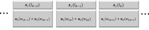
In fact, both MAT and α-MAT can be implemented in a block-Markov fashion, the concept of which is shown in Fig. 1 for α= 0. The common message xc(lb−1)comes from the
previous blockb−1, anduk(wkb)is the new private message
dedicated to Receiverk (k= 1,2). Essentially, we “squeeze” the Phase II of block b−1 and the Phase I of blockb into one single block, with proper power and rate scaling.
𝒙𝑐(𝑙𝑏−2)
𝒖1𝑤1𝑏−1+ 𝒖2(𝑤2𝑏−1)
𝒙𝑐(𝑙𝑏−1)
𝒖1𝑤1𝑏 + 𝒖2(𝑤2𝑏)
𝒙𝑐(𝑙𝑏)
𝒖1𝑤1𝑏+1 + 𝒖2(𝑤2𝑏+1)
[image:6.612.57.294.279.327.2]⋯
⋯
Fig. 1: Block-Markov Encoding.
The transmission consists of B blocks of length n. For simplicity of demonstration, we set n = 1. In block b, the transmitter sends a mixture of two new private messagesw1b
and w2b together with one common message lb−1, for b =
1, . . . , B. As it will become clear, the message lb−1 is the
compression index of the mutual interferences experienced by the receivers in the previous blockb−1. By encodingw1b,w2b,
and lb−1 into u1(w1b), u2(w2b), and xc(lb−1), respectively,
with independent channel codebooks, the transmitted signal is written as
x[b] =xc(lb−1) +u1(w1b) +u2(w2b), b= 1, . . . , B
(16)
where we set l0= 1 to initiate the transmission and w1B = w2B = 1to end it. As before, the common messagexc(lb−1)
is with power P, whereas the precoding inu1 andu2 is with
a reduced power, parameterized byA,A0, with0≤A, A0≤1, such that
Q1=PAΦΦΦˆh2+PA
0 ΦΦΦˆh⊥
2, Q2=P
AΦΦΦ
ˆ
h1+P
A0ΦΦΦ
ˆ
h⊥
1 (17)
whereA,(A0−α)+. The mutual interferences are defined
similarly and their powers are now reduced
y1[b] =hH1xc(lb−1)
| {z }
P
+hH
1u1(w1b)
| {z }
PA0
+hH
1u2(w2b)
| {z }
η1b∼PA
(18)
y2[b] =hH2xc(lb−1)
| {z }
P
+hH
2u2(w2b)
| {z }
PA0
+hH
2u1(w1b)
| {z }
η2b∼PA
(19)
where we omit the block indices for the channel coefficients as well as the AWGN for brevity. At the end of block b,
(η1b, η2b)are compressed with a codebook of sizeP2A into
an indexlb∈
1, . . . , P2A . The distortion between(η1b, η2b)
and(ˆη1(lb),ηˆ2(lb))is at the noise level.
At the end ofB blocks, Receiverk would like to retrieve
wk1, . . . , wk,B−1. Let us focus on Receiver 1, without loss of
generality. In this particular case,lb−1 can be decoded at the
end of block b, by treating the private signals as noise, i.e., with signal-to-interference-and-noise-ratio (SINR) levelP1−A0,
forb= 2, . . . , B. The correct decoding oflb−1is guaranteed if
the SINR can support the DoF of2Afor the common message, i.e.,
2A≤1−A0. (20)
Given that this condition is satisfied,l0, l1, . . . , lB−1 are
avail-able to both receivers. Therefore, η1b, η2b,b = 1, . . . , B−1,
are known, up to the noise level. To decodew1b, Receiver 1
uses η1b,η2b, andlb−1 to form the following 2×2 MIMO
system
y1[b]−hH1xc(lb−1)−η1b η2b
=
hH
1 hH
2
u1(w1b) (21)
where the equivalent channel matrix has rank 2almost surely. This decoding strategy for the private message boils down to the backward decoding, where the mutual interferences (η1b, η2b) decoded in the future block are utilized in current block as
side information. From the covariance matrixQ1 ofu1 from
(17), we deduce that the correct decoding ofw1b is guaranteed
if the DoF d1b ofw1b satisfies
d1b≤A+A0. (22)
Combining (20) and (22), it readily follows that the optimal
A0 should equalize (20), i.e.,A0∗= 1+23α. Thus, we achieve
d1b = 2+3α. Due to the symmetry, d2b has the same value.
Finally, we have
dk= 1 B
B−1
X
b=1
dkb= B−1 B
2 +α
3 , k= 1,2 (23)
which goes to 2+3α when B→ ∞.
By now, we have shown that both MAT andα-MAT schemes can be interpreted under a common framework of block-Markov encoding with power allocation parameters (A, A0)and that they only differ from the choice of these parameters. As we will show in the following subsections, the strength (or benefit) of the block-Markov encoding framework becomes evident in the asymmetric system setting, where the originalα-MAT alignment fails to achieve the optimal DoF in general.
C. Asymmetry in Current CSIT Qualities
Let us consider again the MISO BC case but assume now that the CSIT qualities of two channels are different, i.e.,α16=α2,
whereαk (k= 1,2)is for Receiverk. The signal model is in the exact same form as in (16) with a more general precoding, parameterized byAk,A0k, with0≤Ak, A0k≤1, such that
Q1=PA1ΦΦΦˆh2+P
A01ΦΦΦ
ˆ
h⊥
2
, Q2=PA2ΦΦΦˆh1+P
A02ΦΦΦ
ˆ
h⊥
1
(24)
TABLE I: Parameter Setting for the (2,1,1)BC Case (α1≥α2)
Condition A0
1 A02 Corner Point(d1, d2)
2α1−α2≤1 A
0 1=
1+α1+α2
3 A
0 2=
1+α1+α2 3
2+2α1−α2
3 ,
2−α1+2α2 3
A01= 1+α2
2 A
0
2=α1 (1, α1)
2α1−α2>1 A01=
1+α2
2 A
0 2=
1+α2
2 (1,
1+α2
2 )
- A0
1=α2 A02=
1+α1
2 (α2,1)
compressed up to the noise level with a source codebook of sizePA1+A2. The decoding at both receivers is the same as
before. To decode the common message lb−1 by treating the
private signals as noise, since the SINR isP1−A01 at Receiver 1
and P1−A02 at Receiver 2, the DoF of the common message
should satisfy
A1+A2≤min{1−A01,1−A02}. (25)
Using the common messages lb andlb−1 as side information,
w1b andw2b can be decoded at the respective receivers if
d1b≤A1+A01 and d2b≤A2+A02. (26)
By carefully selecting the parametersA01 andA02, all corner points of the DoF outer bound can be achieved, as shown in Table I on the top of this page where the condition is to make sure the corner points exist. Note that the corner point (α2,1)
always exists as long as α1≥α2.
D. Asymmetry in Antenna Configurations
We use the (4,3,2) MIMO BC case to show that the block-Markov encoding can achieve the optimal performance in asymmetric antenna settings. Recall that, in the previous subsections, the backward decoding is performed to decode the private messages, and that the common messages can be decodedblock by block. In this case, however, we also need backward decoding to decode the common messages as well. The same transmission signal model (16) is used here, with the following precoding, parameterized byAkandA0k,k= 1,2, 0≤Ak ≤A0k≤1:
Q1=PA1ΦΦΦ ˆ
H2+P
A01ΦΦΦ
ˆ
H⊥
2, Q2=P
A2ΦΦΦ ˆ
H1+P
A02ΦΦΦ
ˆ
H⊥
1
(27)
whereAk,k6=j ∈ {1,2}, is defined as
Ak ,
(
(A0k−αj)+, dk≤4−Njαj, dk−(4−Nj)
Nj , dk>4−Njαj
(28)
with dk ∈ R+ being the achievable DoF associated with
Receiver k. It is readily verified that A0k−αj ≤ Ak ≤A0k
is always true, such that the created interference at intended Receiver j is of power level Ak, and the desired signal at Receiverk is of levelA0k.
We recall that the common messagexc(lb−1)is transmitted
with powerP and that the ranks ofΦΦΦHˆ2,ΦΦΦHˆ⊥
2,Φ
ΦΦHˆ1, andΦΦΦHˆ⊥
1
are respectively 2, 2, 3, and 1, almost surely. The received signals are now vectors given by
y1[b] =H1xc(lb−1)
| {z }
PI3
+H1u1(w1b) +H1u2(w2b)
| {z }
η1b∼PA2I3
, (29)
y2[b] =H2xc(lb−1)
| {z }
PI2
+H2u2(w2b) +H2u1(w1b)
| {z }
η2b∼PA1I2
. (30)
Following the same footsteps as in the single receive antenna case, it is readily shown that(η1b,η2b)can be compressed up to the noise level with a source codebook of sizeP2A1+3A2.
For convenience, let us define
dη,2A1+ 3A2. (31)
Unlike the MISO case where the common messages can be decoded independently in each block without loss of optimality, backward decoding is required tojointlydecode the common and private messages in the general MIMO case, in order to achieve the optimal DoF. As we will see later on, the common rate can be improved with backward decoding in general. The decoding starts at blockB. Sincew1Bandw2Bare both known,
the private signals can be removed from the received signals
y1[B]andy2[B]. The common messagelB−1 can be decoded
at both receivers ifdη ≤2. At blockb, forb=B−1, . . . ,2, assuminglbis known perfectly from the decoding of blockb+1,
η1b and η2b can be reconstructed up to the noise level. The
following MIMO system can be obtained
y1[b]−η1b
η2b
=
H1
0
xc(lb−1) +
H1 H2
u1(w1b). (32)
Note that this is a multiple-access channel (MAC) from which
lb−1 and w1b can be correctly decoded if the rate pair lies
within the following region
dη≤3 (33)
d1b≤2A1+ 2A01 (34)
dη+d1b≤3 + 2A1, (35)
whose general proof is provided in Appendix A. Let us set
d1b to equalize (34). Then, (33) and (35) implydη≤3−2A01.
Similar analysis on Receiver 2 will lead to dη≤2−A02, by settingd2b=A02+ 3A2. Therefore, from (31), we obtain the
following constraint
2A1+ 3A2≤min{3−2A01,2−A
0
2} (36)
to achieve any (d1b, d2b)such that
d1b≤2A1+ 2A01 and d2b ≤A02+ 3A2. (37)
By lettingB→ ∞,d1= 2A1+2A10 andd2=A02+3A2can be
achieved for anyA01, A02≤1given the definition of(A1, A2)in
(28), as long as (36) is satisfied. We can show that, by properly choosing (A01, A02), all the corner points given by the outer bound can be achieved. For example, by settingα1=α2=α,
the values(A01, A02)that achieve the corner points are illustrated
in Table II on the top of the next page. Note that(125,45+α)
exists only whenα≤4
5, whereas(3α,4−3α)and(4−2α,2α)
TABLE II: Parameter Setting for the(4,3,2) BC Case withα1=α2=α.
Corner Point(d1, d2) Cond. (A01, A02) (A1, A2) dη
(3, α) α≤
1
2 (
3+2α
4 , α) (
3−2α 4 ,0)
3−2α 2 α >12 (1, α) (12,0) 1
(2α,2) α≤
2
3 (α,
2+3α
4 ) (0,
2−α 4 )
6−3α 4 α >23 (α,1) (0,13) 1
(125,45+α) α≤4
5 (
3 5+
1 2α,
1
5+α) (
3 5−
1 2α,
1 5)
9 5−α (3α,4−3α) α >45 (1,1) (3α2−2,1−α) 1
(4−2α,2α) α >45 (1,1) (1−α,2α3−1) 1
V. ACHIEVABILITY:THEGENERALFORMULATION
As aforementioned, the key ingredients of the achievability scheme consist of:
• block-Markov encoding with a constant block length: the fresh messages in the current block and the interferences created in the past blocks are encoded together with the proper rate splitting and power scaling;
• spatial precoding with imperfect current CSIT: with proper power allocation over the range and null spaces of the inaccurate current channel, the interference power at unintended receiver can be reduced as compared to that without any CSIT;
• interference quantization: instead of forwarding the over-heard interference directly in an analog way as done in pure delayed CSIT scenario, the reduced-power interfer-ences are compressed first with a reduced number of bits, and forwarded in a digital fashion with lower rate; • backward decoding: the messages are decoded from the
last block to the first one, where in each block the messages are decoded with the aid of side information provided by the blocks in the future.
In the following, the general achievability scheme will be described in detail for BC and IC respectively.
A. Broadcast Channels
First of all, we notice that the region (6) given in Theorem 1 does not depend on M (resp.Nk) whenM > N1+N2 (resp.
Nk > M). Therefore, it is sufficient to prove the achievability
for the caseM ≤N1+N2andNk≤M. And the achievability
for the other cases can be inferred by simply switching off the additional transmit/receive antennas. Thus, it yields
M = min{M, N1+N2},
Nk= min{M, Nk}, k= 1,2. (38)
Block-Markov encoding
The block-Markov encoding has the same structure as before, namely,
x[b] =xc(lb−1) +u1(w1b) +u2(w2b), b= 1, . . . , B
(39)
where we recall that we setl0= 1 to initiate the transmission
andw1B=w2B= 1 to end it.
Spatial precoding
Bothu1,u2∈CM×1 are precoded signals ofM streams, such that
Q1=PA1ΦΦΦHˆ2+P
A0
1ΦΦΦ ˆ
H⊥
2
, Q2=PA2ΦΦΦHˆ1+P
A0
2ΦΦΦ ˆ
H⊥
1
(40)
where the rank of ΦΦΦHˆk is Nk whereas the rank of ΦΦΦHˆ⊥
k is
M−Nk,k= 1,2. In other words, for Receiverk,Nj streams
are sent in the subspace of the unintended Receiver j with power levelAk and the other M−Nj streams are sent in the
null space of Receiverj with power levelA0k, where(Ak, A0k)
satisfies
0≤Ak≤A0k ≤1 and Ak≥A0k−αj (41)
forj6=k∈ {1,2}. Note that the above condition guarantees that the interference at Receiverj has power levelAk and the
desired signal at Receiverk is of power levelA0k.
Interference quantization
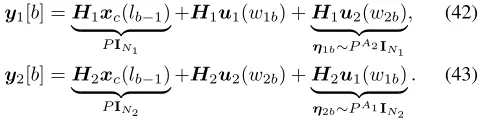
Recall that the common messagexc(lb−1)is sent with power
P. The received signals in blockb are given by
y1[b] =H1xc(lb−1)
| {z }
PIN1
+H1u1(w1b) +H1u2(w2b)
| {z }
η1b∼PA2IN1
, (42)
y2[b] =H2xc(lb−1)
| {z }
PIN2
+H2u2(w2b) +H2u1(w1b)
| {z }
η2b∼PA1IN2
. (43)
It is readily shown that (η1b,η2b) can be compressed up to the noise level with a source codebook of sizePN2A1+N1A2
into an indexlb. For convenience, let us define
dη1 ,N1A2, dη2 ,N2A1, anddη,dη1+dη2. (44)
Backward decoding
The decoding starts at block B. Since w1B and w2B are
both known, the private signals can be removed from the received signalsy1[B]andy2[B]. The common messagelB−1
can be decoded at both receivers ifdη ≤min{N1, N2}. At
blockb, assuminglb is known perfectly from the decoding of
blockb+ 1,η1b andη2b can be reconstructed up to the noise
level, forb=B−1, . . . ,2. The following MIMO system can be obtained at Receiverk,k= 1,2
yk[b]−ηkb
ηjb
=
Hk 0
xc(lb−1) +
Hk
Hj
forj 6=k∈ {1,2}. Since the common messagelb−1 and the
private messagewkbare both desired by Receiverk, this system
corresponds to a multiple-access channel (MAC). As formally proved in Appendix A, Receiverk can decode correctly both messages if the following conditions are satisfied.
dη ≤Nk (46)
dkb≤NjAk+ (M −Nj)A0k (47) dη+dkb≤Nk+NjAk. (48)
Let us choose dkbto be equal to the right hand side of (47)
for k= 1,2 andb = 1, .., B−1. Then, the equality in (47) together with (44), (46), (48) implies, when letting B → ∞, the following lemma.
Lemma 1 (decodability condition for BC). Let us define
ABC,
(A1, A01, A2, A20)|Ak, A0k∈[0,1],
A0k−αj ≤Ak≤Ak0,∀k6=j∈ {1,2} (49)
DBC,{(d1, d2)|dk∈[0, Nk], ∀k∈ {1,2}} (50)
and
fA-d :ABC→ DBC (51)
(Ak, A0k)7→dk,NjAk+ (M−Nj)A0k,∀k6=j∈ {1,2}.
(52)
Then (d1, d2) =fA-d(A), for some A∈ ABC, is achievable
with the proposed scheme, if
dη1+d1≤N1, (53)
dη2+d2≤N2. (54)
where we recall dη1 ,N1A2 and dη2 ,N2A1.
Remark 4. In the above lemma,dηk can be interpreted as the
degrees of freedom occupied by the interference at Receiver k. Therefore, (53) and (54) are clearly outer bounds for any transmission strategies, i.e., the sum of the dimension of the useful signal and the dimension of the interference signal at the receiver side cannot exceed the total dimension of the signal space. These bounds are in general not tight except for special cases such as the “strong interference” regime where interference can be decoded completely and removed or the “weak interference” regime where the interference can be treated as noise while the useful signal power dominates the received power. Remarkably, the proposed scheme achieves these outer bounds. This is due to two of the main ingredients of our scheme, namely, the block-Markov encoding and interference quantization. The block-Markov encoding places the digitized interference in the “upper level” of the signal space (with full power) and thus “pushes” the channel into the “strong interference” regime in which the digitized interference can be decoded thanks to the structure brought by the interference quantization.
Definition 3 (achievable region for BC). Let us define
IBC
A ,
(A1, A01, A2, A02)∈ ABC
(d1, d2) =fA-d(A1, A01, A2, A02),
dk
Nk ≤1−Aj, k6=j∈ {1,2}
(55)
and the achievable DoF region of the proposed scheme
IBC
d ,fA-d(IABC),
(d1, d2)
(d1, d2) =fA-d(A1, A01, A2, A02),
(A1, A01, A2, A02)∈ ABC,
dk
Nk ≤1−Aj, k6=j∈ {1,2}
. (56)
Achievability analysis
In the following, we would like to show that any pair(d1, d2)
in the outer bound region defined by (6), hereafter referred to as OBC
d , can be achieved by the proposed strategy. Therefore,
it is sufficient to show thatOBC
d ⊆ I
BC
d . The main idea is as
follows. If there exists a function
fd-A : OdBC→ ABC (57)
such that
(d1, d2) =fA-d(fd-A(d1, d2)), and (58)
fd-A(d1, d2)∈ IABC, (59)
then for every(d1, d2)∈ OdBCwe can use the power allocation (A1, A01, A2, A20) = fd-A(d1, d2) on the proposed scheme to
achieve it, i.e.,
OBC
d =fA-d(fd-A(OdBC))⊆fA-d(IABC) =I
BC
d (60)
from which the achievability is proved. Now, we define formally the power allocation function.
Definition 4 (power allocation for BC). Let us definefd-A :
OBC
d → ABC:
(d1, d2)7→(A1, A01),f1(d1), (A2, A02),f2(d2) (61)
wherefk,j6=k∈ {1,2}, is specified as below. • WhenM =Nj:Ak0 =Ak= dMk;
• WhenM > Nj anddk < M−Njαj:Ak = (A0k−αj)+,
and thus
A0k=
( d
k
M−Nj, if dk<(M−Nj)αj;
dk+Njαj
M , otherwise;
(62)
• WhenM > Nj and dk≥M−Njαj: A0k= 1, and thus
Ak =
dk−(M−Nj)
Nj .
It is readily shown that, for any (d1, d2) ∈ OBCd , the
resulting power allocation always lies inABC as defined in
(49) and that (58) is always satisfied. It remains to show that (59) holds as well, i.e., the decodability condition in (55) is satisfied. To that end, for any (d1, d2) ∈ OdBC, we
first define (A1, A01, A2, A02) , fd-A(d1, d2) which implies
dj =NkAj+ (M −Nk)A0j,j 6=k∈ {1,2}. Applying this equality on the constraints in the outer boundOBC
d in (6), we
have
dk Nk ≤
M −(M −Nk)A0j
Nk −Aj, (63)
dk Nk
≤1−
(M−N
k)(A0j−αk) +NkAj M
+
for k6=j∈ {1,2}, where the first one is from the sum rate constraint (6c) whereas the second one is from the rest of the constraints in (6). The final step is to show that either of (63) and (64) implies the last constraint in (55):
• When M =Nk, (64) is identical to the last constraint in (55);
• When M > Nk anddj ≥M−Nkαk, we haveA0j = 1
according to the mapping fd-A defined in Definition 4.
Hence, (63) is identical to the last constraint in (55); • When M > Nk and dj < M−Nkαk, we have Aj =
(A0j−αk)+ according to Definition 4. Hence,
(M−N
k)(A0j−αk) +NkAj M
+
≥Aj (65)
with which (64) implies the last constraint in (55). By now, we have proved the achievability through the existence of a proper power allocation function such that (58) and (59) are satisfied for every pair (d1, d2) in the outer bound.
B. Interference Channels
The proposed scheme for MIMO IC is similar to that for BC, with the differences that (a) the interferences can only be reconstructed at the transmitter from which the symbols are sent, and (b) antenna configuration does matter at both transmitters and receivers. Further, as with the broadcast channel, we notice that the region (12) given in Theorem 2 does not depend on
Mk (resp.Nk) whenMk> N1+N2 (resp.Nk > M1+M2),
k= 1,2. Therefore, it is sufficient to prove the achievability for the case Mk ≤N1+N2 and Nk ≤M1+M2, k= 1,2,
since the achievability for the other cases can be inferred by simply switching off the additional transmit/receive antennas. Thus, it yields
Mk = min{Mk, N1+N2},
Nk = min{Nk, M1+M2}, k= 1,2.
(66)
We also define for notational convenience
N10 ,min{N1, M2}, N20 ,min{N2, M1}. (67)
Block-Markov encoding
The block-Markov encoding is done independently at both transmitters
x1[b] =x1c(l1,b−1) +u1(w1b), (68) x2[b] =x2c(l2,b−1) +u2(w2b), b= 1, . . . , B (69)
where we setl1,0=l2,0= 1to initiate the transmission and
w1B =w2B= 1 to end it.
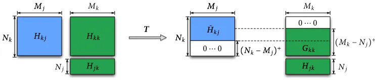
Spatial precoding
The signal uk ∈CMk×1, k = 1,2, is precoded signal of
Mk streams, such that
Q1=PA1ΦΦΦ ˆ
H21+P
A01ΦΦΦ
ˆ
H⊥1 21 +P
A001ΦΦΦ
ˆ
H⊥2
21 , (70)
Q2=PA2ΦΦΦHˆ12+P
A0
2ΦΦΦ ˆ
H⊥1 12
+PA002ΦΦΦ ˆ
H⊥2
12 (71)
where we use Hˆ⊥1
jk (resp. Hˆ
⊥2
jk) to denote any matrix
span-ning the(Mk−Nj0−ξk)-dimensional (resp.ξk-dimensional)
subspace of the null space ofHˆjk whereξk will be specified
later on. Therefore, the rank ofΦΦΦHˆ jk isN
0
j whereas the rank
ofΦΦΦHˆ⊥1 jk and
Φ ΦΦHˆ⊥2
jk are respectively
Mk−Nj0−ξk and ξk, k= 1,2. The power levels(Ak, A0k, A
00
k)satisfy Ak, A0k, A00k∈[0,1],
Ak ≤A0k, A00k ≤Ak0, and Ak ≥A0k−αj
(72)
forj6=k∈ {1,2}. Note that the above condition guarantees that the interference at Receiverj has power levelAk and the desired signal at Receiverk at power levelA0k.
Interference quantization
Recall that the common messages x1c(l1,b−1) and x2c(l2,b−1) are sent with power P. The received signals in
blockb are given by
y1[b] =H11x1c(l1,b−1) +H12x2c(l2,b−1)
| {z }
PIN1
+H11u1(w1b) +H12u2(w2b)
| {z }
η1b∼PA2IN01
, (73)
y2[b] =H22x2c(l2,b−1) +H21x1c(l1,b−1)
| {z }
PIN2
+H22u2(w2b) +H21u1(w1b)
| {z }
η2b∼PA1IN0
2
. (74)
It is readily shown that η1b and η2b can be compressed
separately up to the noise level with two independent source codebooks of size PN10A2 and PN20A1, into indices l
2,b and l1,b, respectively. For convenience, let us define
dη1 ,N10A2, dη2 ,N
0
2A1, anddη,dη1+dη2. (75)
Backward decoding
The decoding starts at blockB. Sincew1B andw2B are both
known, the private signals can be removed from the received signalsy1[B]and y2[B]. The common messages l1,B−1 and
l2,B−1 can be decoded at both receivers if
dηk ≤min{Mj, N1, N2}, (76)
dη1+dη2 ≤min{N1, N2}, (77)
i.e., the common rate pair should lie within the intersection of MAC regions at both receivers for the common messages. At blockb, assuming bothl1,b andl2,bare known perfectly from
the decoding of blockb+ 1,η1b andη2b can be reconstructed
up to the noise level, for b = B−1, . . . ,2. The following MIMO system can be obtained at Receiverk
yk[b]−ηkb
ηjb
=
Hkk 0
xkc(lk,b−1) +
Hkj 0
xjc(lj,b−1)
+
Hkk
Hjk
uk(wkb) (78)
messages l1,b−1, l2,b−1, and wkb are to be decoded. It will
be shown in the Appendix A that the three messages can be correctly decoded if the DoF quadruple(dη1, dη2, d1b, d2b)lies
within the following region
dkb≤Nj0Ak+ (Mk−Nj0−ξk)A0k+ξkA00k
(79)
dηk ≤min{Mj, N1, N2} (80)
dη1+dη2 ≤min{N1, N2} (81)
dηk+dkb≤N
0
k+ min
Mk−Nj0, Nk−Nk0 A0k
+Nj0Ak (82) dηj +dkb≤min{Mk, Nk}+Nj0Ak (83)
dη1+dη2+dkb≤Nk+Nj0Ak. (84)
Now, let us fix
dkb,Nj0Ak+ (Mk−Nj0−ξk)A0k+ξkA00k (85)
dηj ,Nj0Ak (86)
from which we can reduce the region defined by (79)-(84). First, we remove (79) that is implied by (85). Second, (80) is not active as it is implied by (86) and (81). Third, (81) is implied by (84) and (85). Finally, from (86), (83) is equivalent to dkb≤min{Mk, Nk}that is implied by (85). Therefore, by
lettingB→ ∞, we have the following counterpart of Lemma 1 for interference channels.
Lemma 2 (decodability condition for IC). Let us define
AIC,
(A1, A01, A
00
1, A2, A02, A
00
2)
Ak, A0k, A00k∈[0,1]
A0k−αj ≤Ak≤A0k, A00k ≤A0k, ξkA00k ≤Nk0(1−Aj), k6=j∈ {1,2}
(87)
DIC,
(d1, d2)| dk ∈[0,min{Mk, Nk}], ∀k∈ {1,2}
(88)
and
fA-d : AIC→ DIC (89)
(Ak, A0k, A00k)7→dk,Nj0Ak+ (Mk−Nj0−ξk)A0k+ξkA00k,
∀k6=j∈ {1,2} (90)
where
ξk ,
(Mk−Nj0)+−(Nk−N0
k)+, if Ck holds
0, otherwise. (91)
Then (d1, d2) =fA-d(A), for someA∈ AIC, is achievable
with the proposed scheme, if
dη1+d1≤N1, (92)
dη2+d2≤N2. (93)
where we recall dη1 ,N10A2 and dη2 ,N
0
2A1.
Proof: It has been shown that with (86) and (90), only (82) and (84) are active. Withξkdefined in (91), we can verify thatMk−Nj0−ξk = minMk−Nj0, Nk−Nk0 . Thus, from (86), (90), (91), and the last constraint in (87), it follows that
(82) always holds. Finally, the only constraint that remains is (84) that can be equivalently written as (92) and (93).
Definition 5 (achievable region for IC). Let us define
IIC
A ,
(A1, A01, A001, A2, A02, A002)∈ AIC
(d1, d2) =fA-d(A1, A01, A001, A2, A02, A002),
dk
N0
k ≤Nk
N0
k
−Aj, k6=j∈ {1,2}
)
(94)
and the achievable DoF region of the proposed scheme
IIC
d ,fA-d(IAIC),
(d1, d2)
(d1, d2) =fA-d(A1, A01, A001, A2, A02, A002),
(A1, A01, A001, A2, A02, A002)∈ AIC,
dk
N0
k ≤Nk
N0
k
−Aj, k6=j∈ {1,2}
. (95)
Achievability analysis
The analysis is similar to the BC case, i.e., it is sufficient to find a functionfd-A : OIC
d → AICwhere OICd denotes the
outer bound region defined by (12), such that
(d1, d2) =fA-d(fd-A(d1, d2)), and (96)
fd-A(d1, d2)∈ IAIC. (97)
Now, we define formally the power allocation function.
Definition 6 (power allocation for IC). Let us define γk,k6= j∈ {1,2}, as
γk,min
1,Mj−dj ξk
. (98)
Then, we define fd-A : OdIC→ AIC:
(d1, d2)7→
(A1, A01, A001),f1(d1, d2),
(A2, A02, A002),f2(d1, d2)
(99)
wherefk,k6=j ∈ {1,2}, such that (90)is satisfied, and that
• whenMk =Nj0:A00=A0k =Ak= dk
Mk;
• whenMk > Nj0,dk<(Mk−Nj0)γk+Nj0(γk−αj)+:
Ak= (A0k−αj)+, A0k =A00k< γk; (100)
• when Mk > Nj0, dk ≥(Mk−Nj0)γk +Nj0(γk−αj)+,
and γk <1:
Ak= (A0k−αj)+, A0k > A00k=γk; (101)
• when Mk > Nj0, dk ≥(Mk−Nj0)γk +Nj0(γk−αj)+,
and γk = 1:
A0k =A00k= 1. (102)
First, one can verify, with some basic manipulations that,
fd-A(OIC
d ) ⊆ AIC. Second, (96) is satisfied by construction.
Finally, it remains to show that (97) holds as well, i.e., the decodability condition in (94) is satisfied. Since the region OIC
d depends on whether the condition Ck holds, we prove
1) Neither C1 nor C2 holds (ξ1 = ξ2 = 0): For any
(d1, d2) ∈ OdIC, we can define (A1, A10, A001, A2, A02, A002) ,
fd-A(d1, d2)which implies, in this case,
dj =Nk0Aj+ (Mj−Nk0)A0j, j6=k∈ {1,2}. (103)
Applying this equality on the constraints in the outer bound OIC
d in (12), we have
dk N0
k
≤min{max{M1, N2},max{M2, N1}}
N0
k
−(Mj−N 0
k)A0j
Nk0 −Aj, (104) dk
Nk0 ≤
min{Mk, Nk} Nk0 −
min{M
k, Nk} −Nk Nk0
+(Mj−N
0
k)(A0j−αk) +Nk0Aj Mj
+
,
(105)
for k6=j∈ {1,2}, where the first one is from the sum rate constraint (12c) whereas the second one is from the rest of the constraints in (12). The final step is to show that either of (104) and (105) implies the last constraint in (94).
• When Mj =Nk0, (105) implies the last constraint in (94) because min{Mk,Nk}−Nk
Nk ≤0;
• When Mj> Nk0 anddj≥Mj−Nk0αk, we haveA0j= 1
according to the mapping fd-A defined in Definition 6,
sinceγj = 1. Hence, the right hand side (RHS) of (104) is not greater than Nk
N0
k
−Aj, which implies the last constraint in (94);
• When Mj > Nk0 anddj < Mj−Nk0αk, we haveAj = (A0j−αk)+ according to Definition 6 withγj = 1. Since
min{Mk,Nk}−Nk
Nk ≤0, we can show that
min{Mk, Nk} −Nk
Nk +
(Mj−Nk0)(A0j−αk) +Nk0Aj Mj
+
≥min{Mk, Nk} −Nk
Nk
+Aj (106)
with which (105) implies the last constraint in (94).
2) Ck holds (ξk >0, ξj = 0): In this case, it is readily shown, from (90) and (91), that
dk=NjAk+ (Nk−Mj)A0k+ξkA00k, (107)
dj=MjAj. (108)
Applying the mapping dj =MjAj on (12c) results in
dk Nk0 ≤
min{Mk, Nk}
Nk0 −Aj (109)
that always implies dk
N0
k ≤ Nk
N0
k
−Aj. Due to the asymmetry,
we also need to prove that dj
Nj ≤1−Ak. Therefore, the final
step is to show that it can be implied by at least one of the constraints in (12), together with (107) and (108).
• When dk < (Mk−Nj)γk +Nj(γk −αj)+, we have
A0
k = A00k < γk according to (100). Therefore, dk =
NjAk+ (Mk−Nj)A0k, plugging which into (12e), we
obtain
dj Nj ≤
min{Mj, Nj}
Nj −
min{Mj, Nj} −Nj
Nj
+(Mk−Nj)(A
0
k−αj) +NjAk Mk
+
(110)
≤ min{Mj, Nj}
Nj −
min{Mj, Nj} −Nj Nj +Ak
(111)
where the [·]+ in (110) is from the single user bound
(12b); the last inequality is due toAk = (A0k−αj)+and min{Mj,Nj}−Nj
Nj ≤0.
• When dk ≥ (Mk −Nj)γk +Nj(γk −αj)+, we have
A0
k ≥A00k=γk according to (101) and (102).
– Ifγk <1, thenAk00=γk= Mj−dj
ξk anddk = (Nk−
Mj)A0k+Mj−dj+NjAk. Plugging the latter into
(12f), we obtain
dj Nj ≤
min{Mj, Nj} Nj −
min{M
j, Nj} −Nj Nj
+(Nk−Mj)(A
0
k−αj) +NjAk Nk+Nj−Mj
+
(112)
≤min{Mj, Nj}
Nj −
min
{Mj, Nj} −Nj Nj +Ak
(113)
where the[·]+in (112) is from the single user bound (12b); the last inequality is due toAk = (A0k−αj)+
and min{Mj,Nj}−Nj
Nj ≤0.
– Ifγk = 1, then A0k=A00k = 1 anddk=Mk−Nj+ NjAk. Plugging the latter into (12c), we obtain
dj Nj
≤ min{Mk, Nk} −Mk+Nj−NjAk
Nj
(114)
≤1−Ak. (115)
Thus, the last constraint in (94) is shown in all cases. By now, we have proved the achievability through the existence of a proper power allocation function such that (96) and (97) are satisfied for every pair(d1, d2)in the outer bound.
VI. CONVERSE
To obtain the outer bounds, the following ingredients are essential:
• Genie-aided bounding techniques by providing side infor-mation of one receiver to the other one [5], [6];
• Extremal inequalityto bound the weighted difference of conditional differential entropies [29], [30];
• Ergodic capacity upper and lower bounds for MIMO channels with channel uncertainty.
In the following, we first present the proof of outer bound (6d) for MIMO BC and (12d) for MIMO IC, referred to in this section asL4. It should be noticed that both bounds share
the same structure. Then, we give the proof of bound (12f) for the MIMO IC case, referred to in this section asL6, when the
A. Proof of BoundL4
We first provide the outer bounds by employing the genie-aided techniques for BC and IC, respectively, reaching a similar formulation of the rate bounds. With the help of extremal inequalities, the weighted sum rates are further bounded. Finally, the bounds in terms of(α1, α2)are obtained by deriving novel
ergodic capacity bounds for MIMO channels with channel uncertainty.
To obtain the outer bounds, we adopt a genie-aided upper bounding technique reminisced in [5], [6], by providing Receiver 2 the side information of Receiver 1’s messageW1as
well as received signalYn
1 . For notational brevity, we define
a virtual received signal as
¯
yi(t),
Hi(t)x(t) +zi(t) for BC
Hi2(t)x2(t) +zi(t) for IC
(116)
and we also define Xn , {x(t)}n t=1, X
n
i , {xi(t)} n t=1, Yik , {yi(t)}k
t=1, and Y¯ik , {y¯i(t)} k
t=1. Denote also
nn , 1 +nRP
(n)
e where n tends to zero as n → ∞ by
the assumption that limn→∞P
(n)
e = 0.
1) Broadcast Channel: The genie-aided model is a degraded BC Xn → (Yn
1 ,Y2n) → Y1n, and therefore we bound the
achievable rates by applying Fano’s inequality as
n(R1−n)
≤I(W1;Y1n|H
n,Hˆn) (117)
= n
X
t=1
I(W1;y1(t)|Hn,Hˆn,Y1t−1) (118)
= n
X
t=1
h(y1(t)|Hn,Hˆn,Yt−1
1 )
−h(y1(t)|Hn,Hˆn,Y1t−1, W1)
(119)
≤
n
X
t=1
(h(y1(t)|H(t))−h(y1(t)|U(t),H(t))) (120)
≤nN10logP−
n
X
t=1
h( ¯y1(t)|U(t),H(t)) +n·O(1) (121)
n(R2−n)
≤I(W2;Y1n,Y
n
2 , W1|Hn,Hˆn) (122)
=I(W2;Y1n,Y
n
2 |W1,Hn,Hˆn) (123)
= n
X
t=1
I(W2;y1(t),y2(t)|Hn,Hˆn,Y1t−1,Y
t−1
2 , W1)(124)
≤
n
X
t=1
I(x(t);y1(t),y2(t)|Hn,Hˆn,Yt−1 1 ,Y
t−1 2 , W1)
(125)
= n
X
t=1
h(y1(t),y2(t)|Hn,Hˆn,Yt−1 1 ,Y
t−1
2 , W1) (126)
−h(y1(t),y2(t)|x(t),Hn,Hˆn,Yt−1 1 ,Y
t−1 2 , W1)
(127)
≤
n
X
t=1
h(y1(t),y2(t)|Hn,Hˆn,Y1t−1,Y
t−1
2 , W1) (128)
= n
X
t=1
h( ¯y1(t),y2¯ (t)|U(t),H(t)) (129)
where U(t) , nY¯1t−1,Y¯2t−1,Ht−1,Hˆt, W
1
o
for BC and
N10 , min{M, N1}; (120) is from (116) and because (a)
conditioning reduces differential entropy, and (b){y¯1(t),y¯2(t)}
are independent ofHn
t+1 andHˆnt+1, given the past states and
channel outputs; (121) follows the fact that the rate of the point-to-pointM×N1MIMO channel (i.e., between the transmitter
and Receiver 1) is bounded by min{M, N1}logP +O(1);
(123) is due to the independence between W1 andW2; (125)
follows date processing inequality; (128) is obtained by noticing (a) translation does not change differential entropy, (b) Gaussian noise terms are independent from instant to instant, and are also independent of the channel matrices and the transmitted signals, and (c) the differential entropy of Gaussian noise with normalized variance is non-negative and finite.
2) Interference Channel: Given the message and correspond-ing channel states, part of the received signal is deterministic and therefore removable without mutual information loss. Hence, similarly to the BC case, we formulate a degraded channel model, i.e., Xn
2 → Y¯1n,Y¯2n
→Y¯n
1 . By applying
Fano’s inequality, the achievable rate of Receiver 1 and Receiver 2 can be bounded as
n(R1−n)
≤I(W1;Y1n|Hn,Hˆn) (130)
=I(W1, W2;Y1n|Hn,Hˆn)−I(W2;Y1n|W1,Hn,Hˆn)
(131)
≤nN˜1logP−I(W2;Y1n|W1,Hn,Hˆn) +n·O(1) (132)
=nN˜1logP−h(Y1n|W1,Hn,Hˆn)
+h(Y1n|W1, W2,Hn,Hˆn) +n·O(1) (133)
=nN˜1logP−h(Y1n|W1,Hn,Hˆn) +n·O(1) (134)
=nN˜1logP−h( ¯Y1n|Hn,Hˆn) +n·O(1) (135)
≤nN˜1logP−
n
X
t=1
h( ¯y1(t)|Hn,Hˆn,Y¯1t−1,Y¯
t−1
2 )
+n·O(1) (136)
=nN˜1logP−
n
X
t=1
h( ¯y1(t)|U(t),H(t)) +n·O(1) (137)
n(R2−n)
≤I(W2;Y1n,Y2n, W1|Hn,Hˆn) (138)
=I(W2;Y1n,Y2n|W1,Hn,Hˆn) (139)
=I(W2; ¯Y1n,Y¯
n
2 |H
n,Hˆn) (140)
= n
X
t=1
I(W2; ¯y1(t),y¯2(t)|Hn,Hˆn,Y¯1t−1,Y¯
t−1
2 ) (141)
≤
n
X
t=1
I(x2(t); ¯y1(t),y¯2(t)|Hn,Hˆn,Y¯1t−1,Y¯
t−1
2 ) (142)
= n
X
t=1
h( ¯y1(t),y¯2(t)|Hn,Hˆn,Y¯1t−1,Y¯
t−1