problem
.
White Rose Research Online URL for this paper:
http://eprints.whiterose.ac.uk/793/
Article:
Mendes, E.M.A.M. and Billings, S.A. (2001) An alternative solution to the model structure
selection problem. IEEE Transactions on Systems Man and Cybernetics Part A: Systems
and Humans, 31 (6). pp. 597-608. ISSN 1083-4427
https://doi.org/10.1109/3468.983416
[email protected] https://eprints.whiterose.ac.uk/
Reuse
Unless indicated otherwise, fulltext items are protected by copyright with all rights reserved. The copyright exception in section 29 of the Copyright, Designs and Patents Act 1988 allows the making of a single copy solely for the purpose of non-commercial research or private study within the limits of fair dealing. The publisher or other rights-holder may allow further reproduction and re-use of this version - refer to the White Rose Research Online record for this item. Where records identify the publisher as the copyright holder, users can verify any specific terms of use on the publisher’s website.
Takedown
If you consider content in White Rose Research Online to be in breach of UK law, please notify us by
An Alternative Solution to the Model Structure
Selection Problem
Eduardo M. A. M. Mendes and Steve A. Billings
Abstract—An alternative solution to the model structure selection problem is introduced by conducting a forward search through the many possible candidate model terms initially and then performing an exhaustive all subset model selection on the resulting model. An example is included to demonstrate that this approach leads to dynamically valid nonlinear models.
I. INTRODUCTION
I
N THE FIELD of control engineering the task of system identification usually consists of determining a discrete linear or nonlinear mathematical model of a stochastic control system from the measurements of input and output signals. Although today’s literature on parameter estimation schemes is vast, the final product of such schemes is often one single model which hopefully reproduces the system characteristics.In traditional regression analysis, the problem of detecting an appropriate model based upon a subset of the original set of candidates consists of [1]
1) the computational algorithm used to provide information for the analysis;
2) the criterion used to analyze the candidates and select a subset;
3) the estimation of the coefficients in the final model. In [2] it is argued that it is unlikely that there is a single best model but rather several equally good ones. This suggests that an evaluation of a fairly large number of models might be desirable. When only dynamically validated models are of interest, cri-teria which incorporate such information during the process of identification should be used. In the context of neural network models, it has been shown that the minimization of the mean squared errors is likely to be a necessary condition for the model to reproduce the dynamical invariants of the original system, but it is definitely not sufficient [3]. These authors used such a state-ment to justify the utilization of a posteriori tests and to conse-quently verify the model’s validity. In this paper similar tests will be introduced as a tool for selecting not only one single model but a family of models which can adequately reproduce
Manuscript received May 26, 1998; revised June 18, 2001. E.M.A.M. Mendes acknowledges the support of CNPq under Grants 301313/96-2 and 201557/91-6. S. A. Billings acknowledges support from EPSRC. This paper was recommended by Associate Editor E. Page, Jr.
E. M. A. M. Mendes is with Departamento de Eletricidade, Fundação de Ensino Superior de São João Del Rei, São João Del Rei, Brazil (e-mail: [email protected]; [email protected]).
S. A. Billings is with the Department of Automatic Control and Systems Engineering, University of Sheffield, Sheffield, U.K. (e-mail: [email protected]).
Publisher Item Identifier S 1083-4427(01)09756-9.
the desired dynamical invariants of the original system. The pri-mary objective is to show that the use of identification schemes which return many good models is worth exploring.
Many procedures which perform exhaustive search or related approaches have been investigated since the 1960s [e.g., [4]–[7]]. An excellent description of such methods and many others is given in [8]. Typically, these procedures consider all subsets of all sizes, and require that the number of data points is at least as great as the number of regressors (or terms). With these procedures it is possible to obtain the best model of each size. Different criteria have been devised in order to choose the optimal model and related good models. In [9] an algorithm was proposed for searching for all subsets of or less variables out of using the usual -norm of deviations. Whereas Narula and Wellington [10] used the -norm (i.e., minimization of the sum of absolute deviations to find the best models of variables out of a -variable trial model), several authors [1], [8], [11] warned users of such procedures about the computational demands imposed by generating all possible subsets. In [8] it is argued that an exhaustive search for all best fitting subsets is not feasible for trail models with more than 25 terms. Such a pitfall has been used to advocate the use of nonoptimal procedures such as stepwise regression, which often refers to an algorithm proposed by Efroymson [12], and other forward [13] and backward algorithms [See [8], for details]. These procedures are not without problems. In [14] it has been shown that stepwise regression does not always succeed in selecting the best subset of a determined size from a trial model when the chosen criterion is the minimization of the explained variance. The reason for this is that stepwise regres-sion minimizes the increment to explained variance and not explained variance itself. Boyce et al. [14] argued that optimal regression (an exhaustive-like approach) and interdependence algorithms should be applied in place of stepwise regression and principal components analysis insofar as subset selection is concerned.
This paper uses both ideas, that is, forward and exhaus-tive-like searches to select models which can reproduce adequately the dynamical invariants of the system under inves-tigation. Briefly, the procedure adopted here will be to conduct a forward search throughout the many possible candidate terms using the orthogonal estimator (OLS-ERR) [13] and then to use the resultant model to perform a similar procedure to all subset selection procedures. Section II includes some background material. In Section III a justification for performing a second search over the final OLS-ERR model is provided. Section IV describes the second search procedure and reviews the role of information criteria in selecting the trade-off between
complexity and fitting accuracy. An example is provided to demonstrate the benefits of the new approach. The main points of the paper are summarized in Section V.
II. BACKGROUNDMATERIAL
This section reviews the concepts used later in the paper.
A. NARMAX Approach
The nonlinear difference equation model, known as the Non-Linear Auto Regressive Moving Average with eXogenous in-puts (NARMAX) model [15] provides a unified representation for a wide class of nonlinear systems. Leontaritis and Billings [15] showed that several well-known models such as the Ham-merstein, Wiener and bilinear models are special cases of the NARMAX model [16]. This model can represented as follows:
(1)
where
, and output, input and noise, respec-tively;
, and corresponding maximum lags; accounts for possible noise, uncer-tainties, unmodeled dynamics; delay;
some nonlinear function, the form of which is usually unknown. Equation (1) is typically used in identification procedures since
is unknown in practice. Insofar as such procedures are con-cerned, the inclusion of monomials in is mainly to avoid the bias in the parameters.
Because can assume a variety of forms, the identification of nonlinear systems becomes a much more difficult task than the linear counter-part, where the major difficulty is to determine the system order. The uniqueness of the representation was ad-dressed in [17] where the NARMAX model was referred to as the recursive representation of a system.
For many real sampled nonlinear systems, the exact NARMAX models, described by the function in (1), are very difficult to determine. Therefore, it is often necessary to approximate by some function. Polynomial NARMAX models have been shown to be a very good choice [18]. The theoretical justification for using polynomial NARMAX models to represent nonlinear systems have been given in [19]. Being linear-in-the-parameters, the polynomial models can readily be estimated using linear least squares methods as can be seen in Section II-B.
B. Orthogonal Least-Squares Estimator With Structure Detection (OLS-ERR)
In this section the orthogonal least-squares estimator with structure detection proposed by [20] is reviewed. In order to pro-vide a practical application of such an estimator, all explanations will be based upon the estimation of polynomial NARMAX
models. To this end, consider the polynomial NARMAX model based upon (1) in the following form:
(2)
where includes a constant and all the output and input terms as well as all combinations up to degree and time . These terms will henceforth be referred to as process terms. The vector are the parameters of such terms. The matrix and the vector are defined likewise.
will be referred to as noise terms.
Unfortunately (2) is not suitable for estimating the parameters of a polynomial NARMAX model because the noise terms are not known. However the noise sequence can be estimated interactively as
(3)
where is the residual at time and , the prediction of , can be written as
(4)
Finally, substituting (4) into (3) and rearranging the order yields
(5)
where and
. Equation (5) clearly belongs to the linear regres-sion model
(6)
where
data length;
column-vectors which represent process and noise terms;
number of distinct such column-vectors; unknown parameters to be estimated.
is the summation of process terms and noise terms. The extended least squares algorithm [21] consists of estimating the process terms first and then using (3) to obtain the residual sequence. Once the residuals are calculated, the noise terms are incorporated into the matrix and a new set of param-eters is estimated. This process is repeated until the residual sequence converges or a predetermined number of iterations is achieved.
In the orthogonal estimator the parameter estimation is per-formed for a linear-in-the-parameters model which is closely related to (6) and which can be represented as
(7)
where the orthogonal vectors and the parameters are con-structed from (6). The original parameters of the model in (6) can be calculated from the .
As stated before, a great advantage of the orthogonal esti-mator is the possibility of selecting the relevant vectors (terms) as a by-product. To demonstrate this, consider again the onal regression (7). In doing so, it is assumed that the orthog-onal property for holds. Therefore, if (7) is multiplied by itself and the time average is taken, the following equation can be derived:
(8)
The output variance consists of two terms. The first term is the part of the output variance ex-plained by the regressors whereas the second term ac-counts for the unexplained variance. Owing to the orthogonal estimator, the increment toward the overall output variance of each regressor (term or vector) can be computed independently as . Expressing this quantity as a fraction of the overall output variance yields the error reduction error (ERR)
(9)
ERR can be used as a simple and effective means of selecting the most relevant regressors in a forward-regression manner. Therefore, ERR imposes a hierarchy of terms according to their contribution toward the overall output variance.
C. Term Clustering
The deterministic part of a NARMAX model, that is, a NARX model, can be expanded as the summation of terms with de-grees of nonlinearity in the range . Each th-order term can contain a th-order factor in and a
th-order factor in and is multiplied by a coefficient as follows [22]:
(10)
where and the upper limit is
if the summation refers to factors in or for fac-tors in . In discrete models estimated from data gen-erated from nonlinear continuous systems, the term coefficients depend on the sampling time and should therefore be strictly
represented as . However, for the sake
of brevity, the argument is dropped.
If the window of length , defined by the model, is sufficiently short such that
(11)
then (10) can be rewritten as
(12)
Definition II.1 [23]: The constants
in (12) are the coefficients of the term clusters , which contain terms of the form
for and . Such coefficients are
called cluster coefficients and are represented as . Clearly, the set of candidate terms for a NARX model is the union of all possible clusters up to degree .
D. Fixed Points
The fixed points of a map are defined as those points for which and usually constitute the starting point in the analysis of nonlinear systems [24].
Usually the fixed points are computed for the autonomous version of the system under investigation. If the original poly-nomial is nonautonomous, then set ,
so that the only remaining terms are those involving the output. The resultant equation (or model) can be considered as an autonomous polynomial and can therefore be used for calculating the fixed points. All the possible clusters of an autonomous polynomial with degree of nonlinearity are
.
Based upon this definition and using the cluster coefficients, the fixed points of an autonomous polynomial with degree of nonlinearity can be calculated by finding the roots of the fol-lowing “clustered polynomial”
(13)
where is a constant. From (13) it can be seen that an autonomous polynomial with degree of nonlinearity will have fixed points if . It should be pointed out that the fixed points are important in the model structure problem [25].
E. Correlation Tests
In the theory of linear systems, the usual statistical approach to validating identified linear models consists of computing the autocorrelation function of the residuals and the cross-correla-tion funccross-correla-tion between the residuals and the input [26].
this will hold if and only if the following conditions are satisfied [27]:
(14)
where is the Kronecker delta. The overbar indicates mean value and denotes the mathematical expectation. When no input is available, that is, the data are a time series, the following correlations test functions should be used [28]:
(15)
Recently two new correlation functions were introduced in [29] as a solution to increase the discriminatory power of the existent correlation tests (14). These two correlation functions defined in terms of delayed outputs are
(16)
where the constant is defined in [29].
The underlying rationale of the correlation tests (14)–(16) is that for a model to be statistically valid, there should be no pre-dictable terms in the residuals. However, in practice only a finite data length will be available. This implies that confidence bands should be used to reveal if the correlation between variables is significant or not. For large the 95% confidence bands are approximately and any significant correlation will be indicated by one or more points of the function lying outside these bands.
III. JUSTIFICATION FORPERFORMING ASECONDTERMSEARCH
There is a considerable literature on the subject of selection of the “best” subset out of a trial model. As pointed out in the introduction, the majority of procedures used in practice do not take into consideration dynamical characteristics of the system. Instead they rely on statistical measures. In this section an at-tempt to justify a second term search over a predetermined trial model is made. To this end, it is necessary to introduce some important concepts.
The structure of identified models can be characterized in space by a point of coordinates
where is the sampling time, is the number of terms al-lowed in the final model and is the max-imum value between the maxmax-imum values of output and input
lag, respectively. is the usual embedding dimension exten-sively used in the literature. The space defined as above is de-noted model structure space (MSS) [30]. In this reference a sub-region of the MSS is defined where the best estimated models are located in accordance with the free parameters. It has been demonstrated that both , the number of data points, and the noise terms are extremely important and can determine whether an estimated model reproduces the desired dynamical character-istics or not. For instance, it can be shown that a model with 18 process terms and 20 linear noise terms reproduces the double scroll attractor of Chua’s circuit [31]. But if no noise terms were included in the final model, this very same model (structure) ex-hibits a completely different motion. In the light of these simple but striking results, the subregion should always be defined
in terms not only of but also of , the
noise variance and noise terms.
As for the influence of the sampling time on the identification of valid models, the discussion in [32] provides clear evidence that the cautious use of higher degree of nonlinearity can in-crease drastically the number of good models.1 Moreover, such models can have greater than the values specified in [30]. Therefore, it is conjectured that the number of valid models in noise terms is much greater than previ-ously considered. This constitutes the basis of the argument that a second search over a predetermined identified model is worth considering. These results appear to contradict a recent numer-ical experiment conducted in [33]. In this paper models were estimated from data generated by the Lorenz [34] and Rössler [35] equations. They reported that 99% of the estimated models were unstable and that only about 0.04% of the model exhibit some chaotic motions but not which were necessarily valid. The reason for these low figures appears to be the estimation of models with 60 coefficients and no noise terms.
The next example will be used to introduce the concept of model families. Also it will be shown that if the correct number of noise terms is chosen rather large models can be identified.
Example 1: Consider the set of normalized equations (x, y, z) of Chua’s circuit [31]. The equations of motion of such a circuit were used to generate data for identification purposes. The resultant data of the -coordinate sampled at
were then corrupted by white noise so that the signal-noise ratio was approximately 42 dB. The number of data points considered in this analysis was .
To demonstrate that even for a large number of terms a rea-sonably good model can be estimated, certain conditions must be satisfied: 1) where is the upper bound for the number of degrees of freedom (DOF) required to de-scribe the system dynamics and 2) no spurious clusters should be in the final model. To avoid the presence of such clusters, it has been shown that the fixed points and consequently the re-lated clusters can be estimated directly from the data using the procedure of Glover and Mees [36] as described in [37]. Once the true clusters are determined, the next step is to then roughly estimate the value of . This can be done visually for
(a) (b)
(c) (d)
[image:6.612.134.459.58.511.2](e)
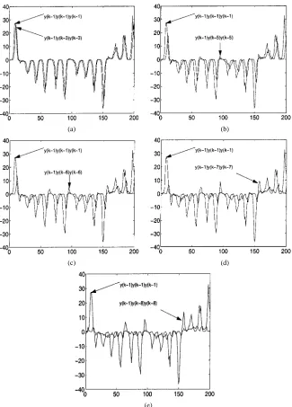
Fig. 1. Estimation ofn using data from thez-coordinate of Chua’s circuit corrupted by white noise, showing plots of the time series generated by different terms of the cluster . The vertical axis is the magnitude of the series whereas the horizontal axis is the number of data points. Note that with only 200 points the maximum lagn can be estimated.
data originated from sampling a continuous-time system. Be-fore showing this procedure, it is worth mentioning that in [30] it is suggested that the lower bound provided by Takens’ the-orem [38] is often larger than necessary [39] and could there-fore be used as an estimate of . The minimum number of degrees of freedom can be obtained, for instance, from estimates of the fractal dimension . is always larger than [40]. Abarbanel et al. have recently devised methods for detecting the minimum embedding dimension [41]. Such a dimension can also be estimated as a by-product of Savit and Green’s procedure [42].
The procedure used to obtain a rough estimate of is
based upon the fact that for
appropriate values of the sampling time . Since the identi-fied models are usually nonlinear, it is conjectured that a sim-ilar relation involving nonlinear terms is also valid. For values
of greater than of this relation is no longer observed. These ideas are better illustrated in Fig. 1(a)–(e). Clearly, it can be seen that terms such as no longer de-scribe a similar trajectory as that of terms like or . This pattern has been observed not only for Chua’s circuit but also for other systems such as Duffing–Ueda [43], Duffing–Holmes [44], etc. From these figures
(a) (b)
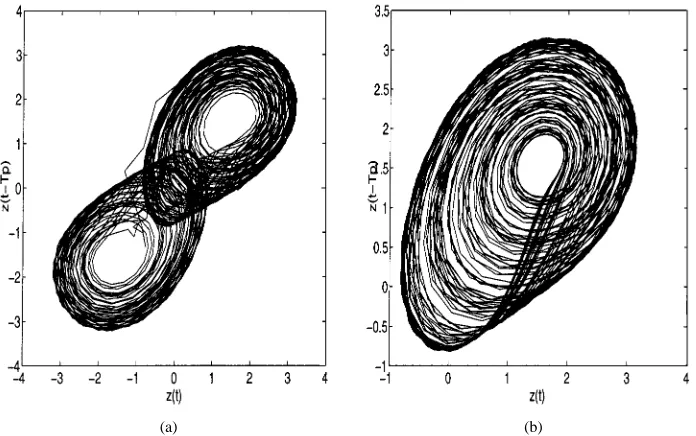
Fig. 2. (a) Double scroll attractor obtained from data generated by the full trial model with one noise term. (b) Spiral-like attractor obtained from data generated by the full trial model with five noise terms.T p = 3 was used.
to produce spurious dynamics because of the presence of extra Lyapunov exponents, as discussed in [37], which causes over-fitting due to the introduction of higher lag terms. These terms also tend to explain the noise in the data.
Taking into consideration all the previous discussion, a trial model with and was chosen. Only linear and cubic terms were allowed due to the attractor’s symmetry detected by Glover and Mees’ procedure. The total number of (process) terms of the resultant trial model is 40 (plus noise terms), that is, all terms were then forced in the regression.
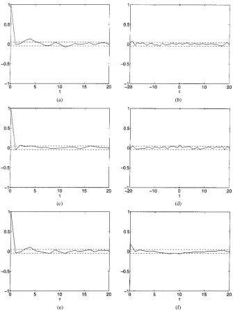
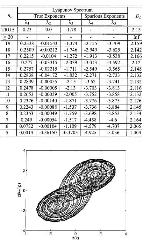
It is important to note that the noise terms play an important role in the determination of the validity of an identified model. For instance, if only a single noise term was included in the trial model reproduces the dynamical invariants fairly well despite the excessive number of terms. Fig. 2(a) shows the double scroll attractor reproduced from the identified trial model. Note how-ever that the noise term is not enough to “bleach” the data and therefore the residuals are correlated [see especially Fig. 3(a)]. As more noise terms are included in the model, it can be observed that 1) all correlation functions lie inside the re-spective confidence bands and 2) several different chaotic mo-tions are registered indicating extreme sensitivity to parameter estimation.2 Fig. 2(b) shows a chaotic motion which resembles the spiral attractor. Table I displays the Lyapunov spectrum for the two models. Note that these models are dimension over-parametrized which can cause a large variety of dynamical be-haviors not exhibited by the original system.
The fixed points of the trial model are
which compares quite well with the fixed points calculated from the equations of Chua’s circuit . When compared to the previous model for the -coordinate of Chua’s circuit, it can be noticed that the location of the fixed points remain al-most constant regardless of the number of terms in the model. Throughout it is assumed that only the effective clusters are
2Theiler and Eubank [46] have shown that the bleaching is more effective when the order of the moving average part(n ) is large.
present in the trial model. It seems that the orthogonal estimator is trying to accommodate the model coefficients in order to pre-serve the location of the fixed points. This becomes more diffi-cult when a large number of terms is involved in the calculation due to ill-conditioning of the numerical solution. The primary problem is not only to obtain a similar location of the fixed points but also stable models. This could be rather difficult to achieve since it has been shown that small variations in parame-ters lead to completely different dynamical behaviors. The same conclusion has been stated in [47] for high dimensional systems. Therefore, variations of the combination of linear and cubic terms could lead to the identification of valid models which were not selected by the OLS-ERR procedure. This statement justi-fies a second search over a model previously identified using such a procedure. Apart from the computational demands im-posed by an exhaustive search, it will be shown that a sub-op-timal procedure can result in better models in cases where the OLS-ERR procedure fails to detect a few good models.
The set of models which exhibits similar characteristics will be denoted as the model family. In the case of models identified from the -coordinate of Chua’s equations the model family is all models with and linear and cubic terms. This constitutes a model family since the fixed points calculated from the model equation for each member are similar and more-over placed near the original fixed points . Several members may exhibit very similar dynamical characteristics and could, therefore, be considered as “optimal” models. This will be illustrated shortly.
IV. SECONDSEARCHPROCEDURE
(a) (b)
(c) (d)
[image:8.612.128.463.58.504.2](e) (f)
Fig. 3. Correlation tests of the residuals(k) originated from the identification of the full trial model. (a) 8 (). (b) 8 (). (c) 8 (). (d)8 (). (e) 8 (). (f) 8 ().
TABLE I
COMPARISONBETWEEN THEORIGINALLYAPUNOVSPECTRUM OFCHUA’S
CIRCUIT ANDTHAT OF THEFULLTRIALMODEL
importance to the variables, an order that may be misleading or confusing, and 2) in the case of early termination, the procedure fails to detect important variables.” Although these problems occurred in such procedures an alternative method using the orthogonal estimator with structure selection [13],
[48]–[50] has been shown to be very efficient in most cases. A similar procedure can be found in [51]. In this case the authors incorporate statistical tests in order to avoid the inclusion of unwanted terms.
An obvious alternative to circumvent the aforementioned problems is to evaluate all possible subsets, that is, to consider all choices of equations involving variables from the original set of variables. The so-called all subset selection procedures are methods of selecting variables that minimize a determined criterion such as the minimum residual sum of squares using some ingenious numerical techniques. These methods have been discussed by several authors and amount to selecting the “best” model from a particular set of variables. For an old but useful review of such methods see [1] and [11].
for determining the subset of each size with minimum residual sum of squares without evaluating all possible regressions. Sev-eral other procedures have been published using the same kernel idea (see for example [6] and [14]). When the number of vari-ables to be selected is very large, the all subset procedures be-come nonviable. This is often the case when trying to fit a non-linear model to data.
In this section a method denoted henceforth as the second search procedure which incorporates the advantage of forward and all subset methods is proposed. Three examples are pro-vided to illustrate the benefits of applying such a procedure. Numerous interesting issues concerning identification are also discussed and solutions are reported. But first, a brief review of some available information criteria is made.
A. Information Criteria
One of the issues when different models structures have been identified is how to compare them and decide which one (or ones) is the best. In statistical terms, the most natural and straightforward method is to evaluate prediction error variances of the different models over new data, that is, data not used for structure selection and parameter estimation. This procedure is called cross-validation [53]. In this method, if a model predicts better over the new data set then it should be considered as the best model.
Ljung and Glad [54] argued that cross-validation always requires a fresh amount of data for model comparison, and therefore not all available information is used for identification. When the model comparison has to be made over the same data used for estimation, a simple prediction error criterion cannot be used. The reason for this is that a larger model always gives a lower variance of prediction errors. Therefore, a trade-off between the number of terms in a model and its capacity to reduce the variance of the prediction errors should be sought. In the field of statistics, this trade-off is achieved by different methods which are, in general, based upon information theoret-ical principles [54]. These methods have similar characteristics, that is, they consist of a determined function which increases with the number of terms and decreases with the number of data points . Minimizing this function with respect to penalizes models which contain an excessive number of parameters or models with large variance of the prediction errors.
The most well-known methods available in the literature are 1) Akaike’s information criterion (AIC) [55]
AIC (17)
2) Final prediction error (FPE) [55]
FPE (18)
3) Khundrin’s law of iterated logarithm criterion (LILC) [56]
LILC (19)
4) Bayesian information criterion (BIC) or Schwarz cri-terion [57]
BIC (20)
5) Rissanen’s minimal description length (MDL) [58]
MDL (21)
In the criteria described above is the variance of the residuals associated to the -term model. Some of the criteria listed above and others available in the literature are just modifications of the AIC criterion [e.g., [57], [59], [60]]. In [61] asymptotic comparisons of some of these criteria has been made. Stone has shown that there is an asymptotic equivalence between cross-validation and AIC. Other criteria such as Mallow’s [62], PRESS [63] and model entropy [64] can also be used as a tool for selecting a model which is a compromise between goodness of fit and complexity. The trade-off model structure is indicated by the value of for which the chosen criterion reached a minimum value. For a review of some of these criteria refer to [65].
Note that the choice of stopping rule depends upon 1) the ob-jectives and 2) the estimation method. In the case of estimation of nonlinear polynomial models, the estimation method used is the orthogonal estimator with structure detection. This estimator imposes an order by which the terms are selected. When calcu-lating an information criterion, the user should be aware that the minimum value depends upon the chosen structure. Varia-tions in this structure will lead to a different choice of number of terms.
The model selection problem using information criteria is still an active field of research. For instance, a new model selection criterion based on the Fisher information matrix was recently proposed in [66]
FIC (22)
where and are the variance of the residuals obtained from the process of identification of a -term model and the full model, respectively.
The quantity can be interpreted as the amount of information in the conditional Fisher matrix defined as . The main property of the Fisher Informa-tion Criteria (FIC) is that the convenInforma-tional penalty term is re-placed by a term that is proportional to the logarithm of the sta-tistical information contained in a -term model.
Despite the good characteristics, the FIC criterion demands heavy computations, when nonlinear models are concerned. For such models, the number of terms can well exceed thousands and therefore the estimation of might lead to spurious results mainly due to ill-conditioned problems. Such problems also oc-curred when criteria such as Mallow’s [62] are used. It is conjectured that the usefulness of criteria which explicitly use the variance of the residuals of the full model is rather limited in nonlinear identification problems.
In Example 1, the second search procedure is performed in order to minimize the difference between the first Lyapunov exponent estimated from the original system and the one cal-culated from the model’s equation estimated directly from the data. The above criterion was adopted to access the validity of the models in terms of dynamical characteristics which cannot be done using the usual information criteria. It will be shown that several models can be identified using such a procedure.
Example 1: Consider again Chua’s circuit equations used in Example 1 presented in Section III to demonstrate that when the model structure is correct even models with a rather large number of terms can reproduce the desired characteristics. A set of 1750 data points without noise contamination were con-sidered to demonstrate the benefits of a second search over a pre-defined set of terms. In this work, this set of terms is always a model estimated using the orthogonal estimator with structure detection.3 Typically, this model contains more terms than are necessary.
The experiment in this example was conducted as fol-lows. Only models with , 10 linear noise terms
and a total number of terms less than 26 were used to define the subregion
noise terms linear . This represents only a fraction of the valid models identified from the data generated by integrating Chua’s equations. A small change in the number of noise terms can lead to valid models which were not considered as such when another noise configuration is adopted.
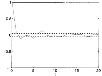
The first step is then to estimate models with increasing com-plexity using the OLS-ERR procedure. A set of 25 models with the number of terms varying from 1 to 25 were identified from the noise-free data of the -coordinate of Chua’s circuit. In [45, p. 858] it is suggested to use 20 linear terms in order to pro-duce unbiased models. These authors stated that the residuals are white and zero-mean with variance . In the case of the noise-free data it is argued that the residuals are not white but simply modeling errors. If schemes such as the procedure discussed in [32] is used to integrate Chua’s equa-tions, these errors are the contribution of terms of degrees of nonlinearity higher than three and cannot, therefore, be consid-ered as white noise. Fig. 4 shows the autocorrelation of the resid-uals obtained from the estimation of a model with 16 process terms and 20 linear noise terms (special case). Clearly the au-tocorrelation function shows some peaks lying outside of the confidence bands. Note that the bleaching effect [46] tends to obscure these peaks.
The dynamical invariants of the models estimated using OLS-ERR procedure were assessed by calculating the Lya-punov dimension and spectrum. These quantities are shown in Table II. The values of the Lyapunov dimension and spectrum for the estimated models demonstrates that only models with and can reproduce fairly well those of the original system. This result is a perfect agreement with those of [45].
The fixed points calculated directly from the equation of the aforementioned models are displayed in Table III. Note that all
[image:10.612.338.512.62.192.2]3Note that in Example 1, 1801 data points were considered. The choice of 1750 was done in order to compare the results presented in this present example with the ones in [45].
Fig. 4. Autocorrelation of the residuals obtained during the process of identification of models from data of thez-coordinate of Chua’s circuit. In this particular case, the model contains 16 process terms and 20 linear noise terms. Variance of residuals is = 8:319 2 10 .
TABLE II
LYAPUNOVEXPONENTS FORMODELSIDENTIFIEDFROMNOISE-FREEDATA. A SINGLETIME-SERIES OF THEz-COORDINATE OFCHUA’SCIRCUIT WAS
CONSIDERED. ALTHOUGHTHERE IS NOCONTAMINATION, TENLINEARNOISE
TERMSWEREALLOWED IN THEFINALMODEL. OLS-ERRWASUSED TO
SELECT THESTRUCTURE ANDESTIMATE THEPARAMETERS
models with from 9 to 24 exhibit the location of fixed points near the true value, that is, which signifies that these models could, in principle, reproduce the desired chaotic behavior. Furthermore the minimum number of terms appears to be , since all models with have fixed points placed far from the correct location.
TABLE III
FIXEDPOINTS FORMODELSESTIMATEDFROM THENOISE-FREEDATA OF THE
z-COORDINATE OFCHUA’SCIRCUIT. OLS-ERRWASUSED TOSELECT THE
STRUCTURE ANDESTIMATE THEPARAMETERS
is repeated until the minimum number of terms chosen a priori is reached.
The results of applying the above procedure are shown in Table IV. Clearly it can be seen that the number of valid (good) models has increased substantially compared to those of Table II. A wide range of models with form 7 to 19 can reproduce the original dynamical invariants. This provides further support to the ideas discussed in the introduction of this paper.
Fig. 5 shows the double scroll attractor reconstructed from the identified model in (23). Despite the small number of terms, this model can reproduce fairly well the desired dynamical in-variants.
(23)
The location of the fixed points for the models estimated using the second search procedure is displayed in Table V. It is interesting to note that the minimum number of terms re-quired for a model to reproduce the original location of the fixed points is now 6. That is, the second search procedures seems to find better models with less terms. These results clearly demon-strate that the sub region consists of a much larger number of valid models than previously expected [30] and moreover that
TABLE IV
LYAPUNOVEXPONENTS FORMODELSIDENTIFIEDFROMNOISE-FREEDATA. A SINGLETIME-SERIES OF THEz-COORDINATE OFCHUA’SCIRCUIT WAS
CONSIDERED. ALTHOUGHTHERE IS NOCONTAMINATION, TENLINEARNOISE
TERMSWEREALLOWED IN THEFINALMODEL. SUBOPTIMALPROCEDURE WAS
[image:11.612.308.546.117.520.2]USED TOSELECT THESTRUCTURE ANDESTIMATE THEPARAMETERS
Fig. 5. Double scroll attractor reconstructed from the data generated by iterating (23).T p = 3 was used.
a second search is well worth the required computational de-mands.
Finally, to illustrate the results presented above in terms of information criteria the AIC criterion was calculated for the models estimated using both procedures, that is, OLS-ERR and the second search procedures. Fig. 6 shows the AIC curves for such models. Note the plateau which ranges from to . These models have been shown to be able to reproduce fairly well the original dynamical invariants, however the resid-uals obtained during the process of estimation of such models exhibit higher variance than those obtained using the OLS-ERR procedure. This shows, not surprisingly, that lower residual vari-ance does not signify better models.
TABLE V
FIXEDPOINTS FORMODELSESTIMATEDFROM THENOISE-FREEDATA OF THE
z-COORDINATE OFCHUA’SCIRCUIT. SUBOPTIMALPROCEDURE WASUSED TO
SELECT THESTRUCTURE ANDESTIMATE THEPARAMETERS
Fig. 6. AIC criterion for estimated models with increasing number of terms. The upper curve shows the values of AIC for estimated models using the second search procedure. Whereas the lower curve shows the values of AIC for estimated models using OLS-ERR procedure.
using the OLS-ERR procedure, a few models are found to be able reproduce the original dynamic invariants of the systema. Despite the initial success of the OLS-ERR procedure, the valid models proved to be unstable when they were iterated for a long time. The use of a second term search lead to better results, that is, stable and dynamically valid models for Rossler equations. Details of the results are available from the authors.
V. CONCLUSION
In this work, an alternative method for solving the model structure selection problem has been proposed and analyzed.
A procedure which combines the advantages of the OLS-ERR and exhaustive-like algorithms has been investigated. Such
a procedure can successfully identify not only a single valid model but a family of models. Such family of models were shown to preserve the desired dynamic characteristics of the original system. It is believed that the results obtained in this paper will help the user of identification techniques, specially when complex nonlinear phenomena such as chaos is of interest. An example has been provided to demonstrate the usefulness of this approach.
As a by-product, a new but simple procedure to determine to maximum lag (embedding dimension) has been devised. This procedure has been used to find the maximum lag for the Chua’s circuit.
It has also been demonstrated that the so-called Information criteria which are extensively used to determine the trade-off be-tween complexity and fitness accuracy can be strongly affected by the inclusion of noise terms. Alternative criteria using dy-namical quantities such as the Lyapunov dimension and spec-trum have been proposed for selecting valid models. The simu-lated example shows the efficacy of such a choice.
REFERENCES
[1] R. R. Hocking, “The analysis and selection of variables in linear regres-sion,” Biometrika, vol. 32, pp. 1–49, Mar. 1976.
[2] J. W. Gorman and R. J. Tomam, “Selection of variables for fitting equa-tions to data,” Technometrics, vol. 8, pp. 27–51, 1966.
[3] J. C. Principe, A. Rathie, and J. M. Kuo, “Prediction of chaotic time series with neural networks and the issue of dynamic modeling,” Int. J.
Bif. Chaos, vol. 2, no. 4, pp. 989–996, 1992.
[4] M. J. Garside, “The best subset in multiple regression analysis,” Appl.
Statistician, vol. 14, pp. 196–200, 1965.
[5] M. Schatzoff, R. Tsao, and S. Fienberg, “Efficient calculation of all possible regressions,” Technometrics, vol. 10, no. 4, pp. 769–779, Nov. 1968.
[6] G. M. Furnival and R. W. Wilson, “Regression by leaps and bounds,”
Technometrics, vol. 16, pp. 499–511, 1974.
[7] D. Edwards and T. Havranek, “A fast model selection procedure for large families of model,” J. Amer. Statist. Assoc., vol. 82, pp. 205–213, 1987. [8] A. J. Miller, Subset Selection in Regression. London, U.K.: Chapman
and Hall, 1990.
[9] A. Kudo and T. Tarumi, “An algorithm related to all possible regression and discriminant analysis,” J. Japan Statist. Soc., vol. 4, pp. 47–56, 1974. [10] S. C. Narula and J. F. Wellington, “Selection of variables in linear re-gression using the sum of weighted absolute errors criterion,”
Techno-metrics, vol. 21, pp. 299–306, 1979.
[11] R. R. Hocking, “Developments in linear regression methodology: 1959–1982 (with discussion),” Technometrics, vol. 25, no. 3, pp. 219–249, Aug. 1983.
[12] M. A. Efroymson, “Multiple regression analysis,” in Mathematical
Methods for Digital Computers, A. Ralston and H. S. Wilf, Eds. New York: Wiley, 1960.
[13] S. A. Billings, S. Chen, and M. J. Korenberg, “Identification of MIMO nonlinear systems using a forward-regression orthogonal estimator,” Int.
J. Contr., vol. 49, no. 6, pp. 2157–2189, 1989.
[14] D. E. O. Boyce, A. Farhi, and R. Weischedel, Optimal Subset
Selec-tion, Multiple Regression, Interdependence and Optimal Network Algo-rithms. New York: Springer-Verlag, 1974.
[15] I. J. Leontaritis and S. A. Billings, “Input–output parametric models for nonlinear systems—Part I: Deterministic nonlinear systems,” Int. J.
Contr., vol. 41, no. 2, pp. 303–328, 1985.
[16] S. A. Billings and I. J. Leontaritis, “Identification of nonlinear systems using parameter estimation techniques,” in Proc. Inst. Elect. Eng. Conf.
Contr. Applicat., Warwick, U.K, 1981, pp. 183–187.
[17] J. Hammer, “Nonlinear systems, stability and rationality,” Int. J. Contr., vol. 40, pp. 1–35, 1984.
[18] S. A. Billings, S. Chen, and R. J. Backhouse, “Identification of linear and nonlinear models of a turbocharged automotive diesel engine,” Mech.
Syst. Signal Process., vol. 3, no. 2, pp. 123–142, 1989.
[20] S. A. Billings, M. Korenberg, and S. Chen, “Identification of nonlinear output-affine systems using an orthogonal least-squares algorithm,” Int.
J. Syst. Sci., vol. 19, no. 8, pp. 1559–1568, 1988.
[21] S. A. Billings and W. S. F. Voon, “Least squares parameter estimation algorithms for nonlinear systems,” Int. J. Syst. Sci., vol. 15, no. 6, pp. 601–615, 1984.
[22] J. C. Peyton-Jones and S. A. Billings, “Recursive algorithms for com-puting the frequency response of a class of nonlinear difference equation models,” Int. J. Contr., vol. 50, pp. 1925–1940, 1989.
[23] L. A. Aguirre and S. A. Billings, “Improved structure selection for nonlinear models based on term clustering,” Int. J. Contr., vol. 62, pp. 569–587, 1995.
[24] J. Guckenheimer and P. Holmes, Nonlinear Oscillations, Dynamical
Systems, and Bifurcation of Vector Fields. New York: Springer-Verlag, 1983.
[25] E. M. A. M. Mendes and S. A. Billings, “On identifying global nonlinear discrete models from chaotic data,” Int. J. Bif. Chaos, vol. 7, no. 11, pp. 2593–2602, Nov. 1997.
[26] T. Söderström and P. Stoica, System Identification. Englewood Cliffs, NJ: Prentice-Hall, 1989.
[27] S. A. Billings and W. S. F. Voon, “Correlation based model validity tests for nonlinear models,” Int. J. Contr., vol. 44, no. 1, pp. 235–244, 1986. [28] S. A. Billings and Q. H. Tao, “Model validity tests for nonlinear signal
processing applications,” Int. J. Contr., vol. 54, no. 1, pp. 157–194, 1991. [29] S. A. Billings and Q. M. Zhu, “Nonlinear model validation using
corre-lation tests,” Int. J. Contr., vol. 60, pp. 1107–1120, 1994.
[30] L. A. Aguirre and S. A. Billings, “Dynamical effects of overparameter-ization in nonlinear models,” Physica D, vol. 80, no. 1 & 2, pp. 26–40, 1995.
[31] L. O. Chua, “Chua’s circuit: An overview ten years later,” J. Circuits,
Syst. Comput., vol. 4, no. 2, pp. 117–159, 1994.
[32] E. M. A. M. Mendes and S. A. Billings, “Discretizing a nonlinear ana-lytic system: Consequences on the model structure problem,” FUNREI Tech Rep., 2001.
[33] G. Rowland and J. C. Sprott, “Extraction of dynamical equations from chaotic data,” Physica D, vol. 58, pp. 251–259, 1992.
[34] E. N. Lorenz, “Deterministic nonperiodic flow,” J. Atmospheric Sci., vol. 20, pp. 131–141, Mar. 1963.
[35] O. E. Rossler, “An equation for continuous chaos,” Phys. Lett. A, vol. 57, no. 5, pp. 397–398, July 1976.
[36] J. Glover and A. I. Mees, “Reconstructing the dynamics of Chua’s cir-cuit,” J. Circuits, Syst. Comput., vol. 3, no. 1, pp. 201–214, 1993. [37] E. M. A. M. Mendes and S. A. Billings, “On overparameterization of
global nonlinear discrete models,” Int. J. Bif. Chaos, vol. 8, no. 3, pp. 535–556, Mar. 1998.
[38] F. Takens, “Detecting strange attractors in fluid turbulance,” in Lecture
Notes in Mathematics, R. A. Rand and L. S. Young, Eds. New York: Springer-Verlag, 1981, vol. 898, pp. 366–381.
[39] D. S. Broomhead, R. Jones, and G. P. King, “Topological dimension and local coordinates for time series data,” J. Phys. A: Math. Gen., vol. 20, pp. L563–L569, 1987.
[40] F. C. Moon, Chaotic Vibrations—An Introduction for Applied Scientists
and Engineers. New York: Wiley, 1987.
[41] H. D. I. Abarbanel and M. B. Kennel, “Local false nearest neighbors and dynamical dimensions from observer chaotic data,” Phys. Rev. E, vol. 47, no. 5, pp. 3057–3068, 1993.
[42] R. Savit and M. L. Green, “Time series and dependent variables,”
Physica D, vol. 50, pp. 95–116, 1991.
[43] Y. Ueda, “Random phenomena resulting from nonlinearity in the system described by Duffing’s equation,” Int. J. Non-Linear Mech., vol. 20, no. 5/6, pp. 481–491, 1985.
[44] P. J. Holmes, “A nonlinear oscillator with a strange attractor,” Phil.
Trans. Roy. Soc. London A, vol. 292, pp. 419–448, 1979.
[45] L. A. Aguirre and S. A. Billings, “Discrete reconstruction of strange attractors in Chua’s circuit,” Int. J. Bif. Chaos, vol. 4, no. 4, pp. 853–864, 1994.
[46] J. Theiler and S. Eubank, “Don’t bleach chaotic data,” Chaos, vol. 4, Dec. 1993.
[47] M. Casdagli, S. Eubank, J. D. Farmer, and J. Gibson, “State space re-construction in the presence of noise,” Physica D, vol. 51, pp. 52–98, 1991.
[48] M. Korenberg, “Orthogonal identification of nonlinear difference equa-tion models,” in Proc. 28th Midwest Symp. Circuits Syst., Louisville, KY, 1985, pp. 90–95.
[49] , “Fast orthogonal identification of nonlinear difference equation and functional expansion models,” in Proc. 30th Midwest Symp. Circuits
Syst., Aug. 1987, pp. 270–276.
[50] M. Korenberg, S. A. Billings, Y. P. Liu, and P. J. McIlroy, “Orthogonal parameter estimation algorithm for nonlinear stochastic systems,” Int. J.
Contr., vol. 48, no. 1, pp. 193–210, 1988.
[51] M. Pottmann, H. Unbehauen, and D. E. Seborg, “Application of a general multi-model approach for identification of a highly nonlinear system—A case study,” Int. J. Contr., vol. 57, no. 1, pp. 197–120, Jan. 1993.
[52] R. R. Hocking and R. N. Leslie, “Selection of the best subset in regres-sion analysis,” Technometrics, vol. 9, pp. 531–540, 1967.
[53] M. Stone, “Cross-validatory choice and assessment of statistical predic-tions,” J. Roy. Statist. Soc. Ser. B, vol. 36, pp. 111–147, 1974. [54] L. Lennard and G. Torkel, “Modeling of dynamic systems,” in
Informa-tion and System Sciences Series. Englewood Cliffs, NJ: Prentice-Hall, 1994.
[55] H. Akaike, “A new look at the statistical model identification,” IEEE
Trans. Automat. Contr., vol. AC-19, pp. 716–723, 1974.
[56] E. J. Hannan and B. G. Quinn, “The determination of the order of an autoregression,” J. R. Statist. Soc. B, vol. 41, no. 2, pp. 190–195, 1979. [57] G. Schwarz, “Estimating the dimension of a model,” Ann. Statist., vol.
6, pp. 416–464, 1978.
[58] J. Rissanen, “Stochastic complexity and modeling,” Ann. Statist., vol. 14, no. 3, pp. 1080–1100, 1986.
[59] H. Akaike, “On entropy maximization principle,” in Applications of
Sta-tistics, P. R. Krishnaiah, Ed. Amsterdam, The Netherlands: North-Hol-land, 1977, pp. 27–41.
[60] J. Rissanen, “Modeling by shortest data description,” Automatica, vol. 14, pp. 465–471, 1978.
[61] M. Stone, “An asymptotic equivalence of choice of model by cross-val-idation and Akaike’s criterion,” J. R. Statist. Soc. Ser. B, vol. 39, pp. 44–47, 1977.
[62] C. L. Mallows, “Some comments onc ,” Technometrics, vol. 15, pp. 661–675, 1973.
[63] D. M. Allen, “Mean square error of prediction as a criterion for selection variables,” Technometrics, vol. 13, pp. 469–475, 1971.
[64] J. P. Crutchfield and B. S. McNamara, “Equations of motion from a data series,” Complex Syst., vol. 1, pp. 417–452, 1987.
[65] J. G. Gooijer, B. Abraham, A. Gould, and L. Robinson, “Methods for determining the order of an autoregressive-moving average process: A survey,” Int. Statist. Rev., vol. 53, no. 3, pp. 301–329, 1985.
[66] C. Z. Wei, “On predictive least squares principles,” Ann. Statist., vol. 20, no. 1, pp. 1–42, 1992.
[67] M. Kortmann and H. Unbehauen, “Two algorithms for model structure determination of nonlinear dynamic systems with applications to indus-trial process,” in Proc. IFAC Symp. Identification Syst. Parameter
Esti-mation, Beijing, China, 1988, pp. 649–656.
[68] A. I. Mees, “Parsimonious dynamical reconstruction,” Int. J. Bif. Chaos, vol. 3, no. 3, pp. 669–675, 1993.
Eduardo M. A. M. Mendes was born in Belo Horizonte, Brazil, in 1964. He received the B.Eng. degree in electrical engineering (with class honors) and the M.Sc. degree from Federal University of Minas Gerais, Belo Horizonte, in 1988 and 1991, respectively. He received the Ph.D. degree in control systems engi-neering from the University of Sheffield, Sheffield, U.K., in 1995.
He was appointed to his current position of Associate Professor, Departa-mento de Eletricidade, Fundação de Ensino Superior de São João Del Rei, São João Del Rei, Brazil, in 1996. His research interests include system identifica-tion for nonlinear systems, narmax methods, model validaidentifica-tion, predicidentifica-tion, spec-tral analysis and chaos.
Steve A. Billings was born in Staffordshire, U.K., in 1951. He received the B.Eng. degree in electrical engineering (first class honors) from the University of Liverpool, Liverpool, U.K., the Ph.D. degree in control systems engineering from the University of Sheffield, Sheffield, U.K., and the D.Eng. degree from the University of Liverpool, in 1972, 1976, and 1990, respectively.
He was appointed to his current position of Professor, Department of Au-tomatic Control and Systems Engineering, University of Sheffield, in 1990 and leads the Signal Processing and Complex Systems Research Group. His research interests include system identification and information processing for nonlinear systems, narmax methods, model validation, prediction, spectral analysis, adap-tive systems, nonlinear systems analysis and design, neural networks, machine vision, spatio-temporal systems and brain imaging.