A fast and robust algorithm to count topologically persistent holes in noisy clouds
Vitaliy Kurlin
Durham University
Department of Mathematical Sciences, Durham, DH1 3LE, United Kingdom
[email protected], http://kurlin.orgAbstract
Preprocessing a 2D image often produces a noisy cloud of interest points. We study the problem of counting holes in noisy clouds in the plane. The holes in a given cloud are quantified by the topological persistence of their boundary contours when the cloud is analyzed at all possible scales.
We design the algorithm to count holes that are most persistent in the filtration of offsets (neighborhoods) around given points. The input is a cloud ofnpoints in the plane without any user-defined parameters. The algorithm has
O(nlogn)time andO(n)space. The output is the array (number of holes, relative persistence in the filtration).
We prove theoretical guarantees when the algorithm finds the correct number of holes (components in the com-plement) of an unknown shape approximated by a cloud.
1. Introduction: counting holes in noisy clouds
We apply methods from the new area of topological data analysis to counting persistent holes in a noisy cloud of points. Such a cloud can be obtained by selecting inter-est points in a gray scale or RGB image. Our region-based method uses global topological properties of contours.By ashapewe mean any subset X ⇢ R2 that can be split into finitely many (topological) triangles. Hence X
is bounded, but may not be connected. Then ahole in a shapeX ⇢ R2is a bounded connected component of the complementR2 X. Such a hole can be a disk, a ring or may have a more complicated topological form, see Fig.1.
The↵-offsetX↵is the union[
p2XB(p;↵)of disks with
the radius↵ 0and centers at all p 2 X. For instance, X0is the original shapeX ⇢ R2. When↵is increasing, the holes ofR2 X↵are shrinking, may split into smaller
newborn holes and will eventually die, each at its own death time↵, see Fig.3. Thepersistenceof a hole is its life span death birthin the filtration{X↵
[image:1.612.310.547.232.324.2]}of all↵-offsets. So we quantify holes by their persistence at different scales↵.
Figure 1. The orange shapeX⇢R2with 3 white holes of
differ-ent forms: a small disk, a ring-like hole, a ‘figure-eight’ hole.
Hole counting problem. Let a shapeXbe represented by
a finite sampleCof points inR2. Find conditions onXand its sample when one can quickly count persistent holes.
We solve the problem by the algorithm HOCTOP : Hole Counting based on Topological Persistence. The only input is a finite cloudCof npoints approximating an unknown shapeX ⇢ R2. The algorithm outputs the relative persis-tence ofkholes in the filtration{C↵
}for allk 0. If the scale↵is random and uniform, this output gives probabili-tiesP(kholes). The boundary edges of persistent holes can be quickly post-processed to extract all boundary contours.
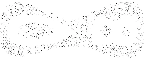
Figure 2. Input: cloudCof 1251 points uniformly sampled from the shape with 3 holes in Fig.1. Output probabilities of HOCTOP : P(3 holes)⇡24%,P(2 holes)⇡13%,P(8 holes)⇡11%.
Theorems1,4say that the algorithm HOCTOP quickly and correctly finds all persistent holes using only a good enough sampleCof an unknown shapeX, see section2.
This is the full 10-page version of the paper published in Proceedings of
[image:1.612.309.543.524.626.2]2. Main results: the algorithm and guarantees
We start from a high-level description of our algorithm. The topological persistence of contours in the filtra-tion{C↵}is computed by using a Delaunay triangulation Del(C)of a given cloudC ⇢ R2 of npoints. By Nerve Lemma8the↵-offsetsC↵can be continuously deformed
to the↵-complexesC(↵), which filterDel(C)as follows:
[image:2.612.51.287.202.322.2]C = C(0) ⇢ · · · ⇢ C(↵) ⇢ · · · ⇢ C(+1) = Del(C). EachC(↵)has some edges and triangles fromDel(C).
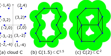
Figure 3. The big hole in the green offsetC↵is born at↵= 1.5,
splits into 2 smaller holes at↵= 2and dies at↵⇡2.577, so the topological persistence of this hole isdeath birth⇡1.077.
The graph dual to Del(C)is filtered by the subgraphs
C⇤(↵) whose connected components correspond to holes inC(↵). When↵is decreasing,C(↵)is shrinking, so its holes are growing and corresponding components ofC⇤(↵) merge at critical values of↵, see Fig.6. The persistence of cycles in the filtration{C↵
}corresponds to the persistence of components in{C⇤(↵)}, see Duality Lemma14.
The pairs (birth,death) of connected components in
{C⇤(↵)} are found via a union-find structure by adding edges and merging components. So computing the 1-dimensional persistence of cycles in {C↵
} reduces to the 0-dimensional persistence of components in{C⇤(↵)}.
Starting from a given cloudC⇢R2ofnpoints with real coordinates(xi, yi),i= 1, . . . , n, we find a Delaunay
trian-gulationDel(C)inO(nlogn)time withO(n)space. Then we remove each edge ofDel(C)one by one in the decreas-ing order of their length. Removdecreas-ing an edge may break a contour when adjacent regions inC(↵)and the correspond-ing components ofC⇤(↵)merge. In the case of a merger, a younger component ofC⇤(↵)and the corresponding hole inC(↵)die. We note thebirth anddeathof each dead hole. We get the probability ofkholes as the relative length
of all intervals of the scale↵whenC↵⇢R2haskholes.
Theorem 1. The algorithm HOCTOP counts all holes in a given cloudC ⇢R2ofnpoints inO(nlogn)time with
O(n)space. All holes are ordered by their topological per-sistence in the ascending filtration{C↵}of the↵-offsets.
Definition 2 ("-sample). A cloud C is an "-sample of a shapeX ⇢ R2if X ⇢ C↵ andC ⇢ X↵. So any point
of C is within the distance " from a point of X and any
point ofXis at most"away from a point ofC. Hence"can be considered as the upper bound of some arbitrary noise.
Definition 3(min and max homological feature sizes). For any shapeX ⇢ R2, let↵ = minhfs(X)be the minimum homological feature sizewhen a first hole is born or dies inX↵. Let↵= maxhfs(X)be the maximumhomological
feature sizeafter which no holes are born or die inX↵.
Theorem 4 gives sufficient (not necessary) conditions when the algorithm finds the correct number of holes in an unknown shape X ⇢ R2 that is represented by its finite sampleC. We extend the Homology Inference Theorem [4] to the case when the upper bound"of noise is unknown.
Theorem 4. Let a cloudCbe an"-sample of a shapeX ⇢
R2with an unknown parameter"such thatminhfs(X)> 1
2maxhfs(X) + 4". If no new holes are appear inX
↵when
↵is increasing, then the algorithmHOCTOP finds the cor-rect number of holes inXby using only the cloudC.
The conditionminhfs(X)> 1
2maxhfs(X) + 4"means that all holes ofX, which are bounded components ofR2
X, have comparable sizes (neither tiny nor huge).
Even if the conditions of Theorem4are not satisfied, we can always find the numberkof holes with the highest prob-ability. The algorithm HOCTOP can also accept a signal-to-noise ratio ⌧ and output all holes whose persistence is larger than⌧. Alternatively, the user may prefer to get most likely outputs ordered by the probabilityP(kholes).
3. Previous work on computing persistence
The offsets C↵of a finite cloud C are usually studiedthrough the ˘Cech or Rips complexes, which may contain up toO(nk) simplices in all dimensionsk
n 1even if
C ⇢R2. A Delaunay triangulation has the advantage of a smaller size up tom=O(n2)in dimensionsn= 2,3,4.
The fastest algorithm [8] for computing persistence of a filtration in all dimensions has the same running time
O(m2.376)in the numbermof simplices as the best known time for the multiplication of twom⇥mmatrices.
In dimension 0 the persistence can be computed in al-most linear time [6, p. 6–8], which was used for simplifying functions on surfaces [1] and for approximating persistence of an unknown scalar field from its values on a sample [3].
4. Delaunay triangulation and
↵
-complexes
Definition 5(simplicial complex). Asimplicial 2-complex is a finite set of simplices(vertices, edges, triangles):•the sides of any triangle are included in the complex;
•the endpoints of any edge are included in the complex;
•two triangles can intersect only along a common edge;
•edges can meet only at a common endpoint (a vertex);
•an edge can not pierce through the interior of a triangle.
If a complexSis drawn inRnwithout self-intersections,
we may call this image|S|ageometric realizationofS. We
have defined a shapeX ⇢R2as a geometric realization of a 2-complex. For instance, a round disk whose boundary is split into 3 edges by 3 vertices is a topological triangle.
Acyclein a complex is a sequence of edgese1, . . . , em
such that any consecutive edgesei, ei+1(in the cyclic order) have a common vertex. Any loop in a geometric realization
|S|continuously deforms to a cycle of edges inS.
Definition 6(Delaunay triangulationDel). For a pointpiin
a cloudC={p1, . . . , pn}⇢R2, theVoronoi cellV(pi) =
{q2R2:d(p
i, q)d(pj, q)8j6=i}is the set of all points
qthat are (non-strictly) closer topithan to other points of
C. TheDelaunay triangulationDel(C)is the nerve of the Voronoi diagram[p2CV(p). Namely,p, q, r 2 C span a
triangle if and only ifV(p)\V(q)\V(r)6=;.
By another definition [2, section 9.1] the circumcircle of anyDelaunay triangleinDel(C)encloses no points ofC.
For a cloudC⇢R2ofnpoints, letDel(C)havek trian-gles andbboundary edges in the external region. Counting
allE edges over triangles, we get 3k+b = 2E. Euler’s
formulan E+ (k+ 1) = 2implies thatk= 2n b 2,
E= 3n b 3. SoDel(C)hasO(n)edges and triangles.
Definition 7 (↵-complex C(↵)). For a scale parameter ↵>0, the↵-complexC(↵)is the nerve of[p2C(V(p)\
B(p;↵)), see [6, section III.4]. Pointsp, q 2 C are
con-nected by an edge ifV(p)\B(p;↵)meetsV(q)\B(q;↵). Three pointsp, q, r 2Cspan a triangle if the intersection
V(p)\B(p;↵)\V(q)\B(q;↵)\V(r)\B(r;↵)6=;.
If↵ > 0 is very small, all points of C are disjoint in C(↵), whileC(↵) = Del(C)for any large enough↵, see examples in Fig.3. So all↵-complexes form the filtration
C = C(0) ⇢ · · · ⇢ C(↵) ⇢ · · · ⇢ C(+1) = Del(C). Edges or triangles are added only atcritical valuesof↵.
Lemma 8(Nerve of a ball covering [5]). The union of balls
C↵ = [
p2CB(p;↵)continuously deforms to (has the
ho-motopy type of) a geometric realization ofC(↵).
5. Persistent homology: definitions, examples
Definition 9 (1-dimensional homologyH1). We consider the 1-dimensional homology groupH1(S)only with coeffi-cients inZ/2Z ={0,1}. Cycles of a 2-dimensional com-plexScan be algebraically written as linear combinations
of edges (with coefficients0or1) and generate the vector spaceC1of cycles. The boundaries of all triangles inS(as cycles of 3 edges) generate the subspaceB1 ⇢ C1. The quotient groupC1/B1is thehomologygroupH1(S).
By a filtration {S(↵)} we mean a sequence of nested complexesS(0) ⇢· · · ⇢S(↵)⇢ . . . that change only at
finitely manycritical values↵1, . . . ,↵m. Then we get the
induced linear mapsH1(S(↵1))!· · ·!H1(S(↵m)). Definition 10 (persistence diagramPD{S(↵)}). In a fil-tration {S(↵)}a homology class 2 H1(S(↵i))isborn
at↵i = birth( )if is not in the image ofH1(S(↵)) !
H1(S(↵i))for any↵ < ↵i. The class diesat the first
time ↵j = death( ) ↵i when the image of
un-der H1(S(↵i)) ! H1(S(↵j)) merges into the image of
H1(S(↵)) ! H1(S(↵j))for some↵ < ↵i. The class
has thepersistencedeath( ) birth( ). The point(↵i,↵j)
has the multiplicityµijequal to the number of independent
classes that are born at↵i and die at↵j. Thepersistence
diagramPD{S(↵)}in{(x, y)2R2 :x
y}is the
multi-set consisting of all points(↵i,↵j)with the multiplicityµij
and all diagonal points(x, x)with the infinite multiplicity. Pairs with a low persistencedeath birth(close to the diagonal{x=y}inPD) are treated as noise. Pairs with a high persistence represent persistent cycles in{S(↵)}.
We shall consider the filtrations of↵-offsets{X↵}and
{C↵
}for a shapeX ⇢R2and a finite cloudC
[image:3.612.307.547.504.586.2]⇢R2. Fig-ures4and5show the persistence diagramPDfor the filtra-tion of the↵-offsetsC↵equivalent toC(↵)by Lemma8.
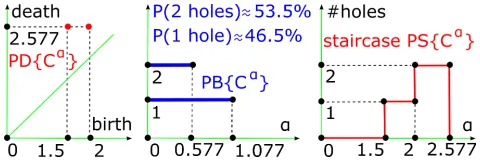
Figure 4. Extra outputs for the cloudCof 10 points in Fig.3. Left: persistence diagram, middle: barcode, right: persistence staircase.
We can convert the persistence diagram into the persis-tence barcodePB{C↵}. All pairs(birth,death)give
hori-zontal bars ordered by their lengthdeath birth. Usually the bars are drawn from the left endpoint0to the right end-pointdeath birth, see the middle picture in Fig.4.
Figure 5. Extra outputs for the cloudCof 1251 points in Fig.2. Left: persistence diagramPD, middle: barcodePB, right: staircasePS.
birth ↵<deathandf(↵) = 0otherwise. The sum of these functions over all pairs gives thepersistence staircase PS{C↵
}. The value of this piecewise constant function of
↵is the number of holes in the offset C↵. We have
con-nected consecutive horizontal segments ofPS{C↵}to get a
‘continuous’ staircase as in the right picture of Fig.4. For the cloudC of 10 points in Fig. 3, the full range of the scale↵is from the smallest critical value↵ = 1.5 (when a first hole is born) to the largest critical value↵=
5 8
p
17 ⇡ 2.577 (when both final holes die). The output probabilityP(1 hole) ⇡ 46.5% is the contribution of the interval(1.5,2)to the full range1.5 ↵ 5
8
p
17. The largest probabilityP(2 holes)⇡53.5%is the contribution of the interval(2,58p17)whenC↵has exactly 2 holes.
For the cloud C of 1251 points in Fig. 2, we scaled
PB{C↵}andPS{C↵}along the horizontal↵-axis and kept only the longest bars in the barcodePB{C↵
}in Fig.5.
6. Persistent homology: stability and duality
Definition 11(bottleneck distancedB). Let the distance
be-tweenp = (x1, y1),q = (x2, y2)inR2 be||p q||1 = max{|x1 x2|,|y1 y2|}. The bottleneck distance is
dB(D, D0) = inf'supp2D||p '(p)||1over all bijections ':D!D0between persistence diagramsD, D0.
Theorem 12. [4] If a finite cloudCof points is an"-sample of a shapeX ⇢R2, thend
B(PD{X↵},PD{C↵})".
Stability Theorem12implies for barcodesPBthat the endpoints of all bars are perturbed by at most". So a long bar can become only a bit shorter after adding noise.
To every triangle in the Delaunay triangulationDel(C), let us associate a single abstract vertexvi,i= 1, . . . , k. It
will be convenient to call the external region ofDel(C)also a ‘triangle’ and represent it by an extra vertexv0.
Definition 13(graphsC⇤(↵)). For any verticesv
i, vj
rep-resenting adjacent triangles inDel(C), letdijbe the length
of the (longest) common edge of the triangles. The metric graphC⇤dual toDel(C)has the verticesv
0, v1, . . . , vkand
edges of the lengthdij connecting verticesvi, vj that
rep-resent adjacent triangles, see Fig.6. The graphC⇤ is fil-tered by the subgraphsC⇤(↵)that have only the edges of a lengthdij>2↵. We remove any isolated nodev(exceptv0) fromC⇤(↵)if the corresponding triangleTvis not acute or
has a smallcircumradiusrad(v)↵. We get the filtration
C⇤=C⇤(0) · · · C⇤(↵) · · · C⇤(+1) ={v0}.
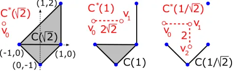
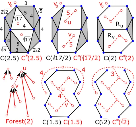
Figure 6. The complexesC(↵)have solid edges and gray triangles. The graphsC⇤(↵)have circled vertices and red dashed edges.
Components of C⇤(↵) are called white, because they represent regions inR2 C(↵)(or holes inR2 C↵). A
cycle ⇢C(↵)is called acontourif bounds a region in R2 C(↵), so ‘encloses’ the corresponding white compo-nent ofC⇤(↵). Lemma14is an analogue of the Symmetry Theorem [6, p. 164] for a function on a closed manifold.
Lemma 14 (Duality). All contours of the complex C(↵) are in a 1-1 correspondence with all connected components of the graphC⇤(↵)not containing the vertexv
0. When↵is decreasing, the contours ofC(↵)and the white components ofC⇤(↵)have the corresponding critical moments:
•a birth of a contour$a birth of a white component,
[image:4.612.309.547.402.476.2]7. The algorithm H
OCT
OP for counting holes
We build the union-find structureForest(↵)on the ver-tices of the graphC⇤(↵). All nodes and trees ofForest(↵) will be in a 1-1 correspondence with all vertices and white components ofC⇤(↵). Every nodevinForest(↵)has
•a pointer to a unique parent of the nodevinForest(↵);
•a pointer to the Delaunay triangle dual to the nodev;
•the weight (the number of nodes belowvin its tree); •the critical value (birth)↵v= sup{↵:v2C⇤(↵)}.
If a nodevis a self-parent, we callvaroot. We can find
root(v)of any nodevby going up along parent links. If↵is decreasing,↵vcan be considered as the birth time when the
vertexvjoinsC⇤(↵). The algorithm initializesForest(↵) as the set of isolated nodesv0, . . . , vk. If the triangle
cor-responding tovk is acute, the birth time ofvk is the
cir-cumradius of the triangle, otherwise 0. We will go through all edges ofDel(C)in the decreasing order of their length and will update ↵v whenv enters the ascending filtration
{v0}=C⇤(+1)⇢· · ·⇢C⇤(↵)⇢· · ·⇢C⇤(0) =C⇤. All triangles of C(↵) and the corresponding nodes of Forest(↵)are calledgray. The remaining triangles and the external region of Del(C)are called white. The external region has birth time+1and is called a ‘triangle’ for sim-plicity. Initially all triangles with birth time 0 are gray.
The while loop. For each edge e ⇢ Del(C)arriving in the decreasing order of length, we find two trianglesTu, Tv
attached toeand check if they are gray or white. To
deter-mine if a triangleTvrepresented by a nodevis gray, we go
up along parent links fromvtoroot(v). If the birth time of root(v)is 0, the triangleTvis still gray, otherwise white.
To distinguish Cases 1 and 4 below, we also check if the triangles Tu, Tv attached to the current edge e are in the
same region ofR2 C(↵). Case 1 means that the nodes
u, v 2 Forest(↵) belong to the same tree, soroot(u) = root(v). In all 4 cases the scale↵goes down through the half-length1
2length(e)of the current edgeefromDel(C).
Case 1:ehas the same white region on both sides ofe.
C(↵)loses only the open edgee. The white components of C⇤(↵)are unchanged. Fig.6illustrates Case 1 for↵ = 1 whenC(↵)loses the edge connecting(1,0)to(1,2).
Case 2: the edgeeis in 1 gray triangle and 1 white triangle. Letu, v 2 C⇤(↵)be the vertices dual to the gray triangle
Tuand the white triangleTvattached to the current edgee
inDel(C). Then the birth times are↵u= 0,↵root(v)>0. Since ↵ is decreasing, the descending filtration C(↵) loses the (open) edgeeand the gray (open) triangleTu. So
the vertexubecomes connected by an edge withvand joins the white component ofC⇤(↵)containingv. Then we link the isolated nodeuto the tree containing the older nodev
inForest(↵). Soroot(v)becomes the parent ofuand the
[image:5.612.309.548.122.346.2]weight ofroot(v)jumps by 1. Fig.7illustrates Case 2 for ↵= p217 whenC(↵)loses the 2 edges of lengthp17.
Figure 7. ComplexesC(↵)and graphsC⇤(↵)are shown for the cloudCfrom Fig.3. Two trees inForest(↵)merge at↵= 2.
Case 3: the edgeeis in the boundary of 2 gray triangles. Let u, v 2 C⇤(↵) be the vertices dual to the gray tri-angles Tu, Tv attached to the current edge e ⇢ Del(C).
ThenTu, Tvare right-angled triangles with the common
hy-potenusee. The birth time of bothu, vis the half-length of e. Since↵is decreasing,C(↵)loses the (open) edgeeand
both (open) trianglesTu, Tv. The contour@(Tu[Tv)
ap-pears inC(↵). So we link the nodesu, vinForest(↵).
Case 4:ehas 2 different white regions on both sides. Let u, v 2 C⇤(↵)be the vertices dual to the white trian-glesTu, Tv attached to the current edgeeinDel(C). The
descending filtration{C(↵)}loses the (open) edgee. The
verticesu, v become connected by an edge, so their white
components inC⇤(↵)merge into a new big component. By Duality Lemma14, two contours enclosing regionsRuand
Rvlose their common edgeeand we get one larger contour @(Ru[Rv)enclosing both regions. Fig.7illustrates Case 4
for ↵ = 2 when C(↵) loses the middle edge of length 4. Then 2 white components (containing 4 vertices each) merge in the graphC⇤(↵)shown after merger at↵= 1.5.
white component Rv dies and we get (birth,death) = (12length(e),↵root(v))for the life of the white component
in the ascending filtration{C⇤(↵)}and of the correspond-ing contour in the descendcorrespond-ing filtration{C(↵)}.
We swapped the birth and death times, because the per-sistence is usually defined when the scale↵is increasing. However, we need the ascending filtration{C⇤(↵)}to use a union-find structure, so↵is decreasing in the algorithm.
Finally, to merge the trees with root(u),root(v) in Forest(↵), we compare the weights of the roots and set the root of the (non-strictly) larger tree as the parent for the root of another tree. So the size of any subtree grows by a factor of at least 2 each time when we pass to the parent. We get
Lemma 15. By the above construction the longest path in any tree of sizekfromForest(↵)has lengthO(logk).
8. Proofs of main results and our conclusion
Proof of Theorem 1. Constructing the Delaunay triangu-lation Del(C) on a cloud ofnpoints requires O(nlogn) time [2, Chapter 9]. SortingO(n)edges ofDel(C)needs
O(nlogn)time. Then we go through thewhile loop ana-lyzing each of the O(n) edges ofDel(C). For the nodes
u, v 2 Forest(↵)of triangles attached to each edgee, we
find the roots of u, v by going up along O(logn)parent links by Lemma15. All other steps in thewhile looprequire onlyO(1)time. Hence the total time isO(nlogn). The sizes of all data structures are proportional to the numbers of edges or triangles inDel(C), so we useO(n)space.
The careful analysis of a union-find structure says that Forest(↵)can be built in timeO(nA 1(n, n))time, where
A 1(n, n)is the extremely slowly growing inverse Acker-mann function. Our time O(nlogn) is dominated by the construction ofDel(C)and sorting allO(n)edges.
Proof of Theorem4.The important critical values of↵for the 1-dimensional homology of the filtration{X↵
}are •↵= minhfs(X)is the 1st value whenH1(X↵)changes;
•↵= maxhfs(X)is the last value whenH1(X↵)changes.
No new holes appear in offsets X↵ of the shape X
with originalkholes. ThenPD{X↵
}contains only points
(0, di). The smallest death isd1= minhfs(X). The largest death isdk = maxhfs(X). If a cloudCis an"-sample of
a shapeX⇢R2, the perturbed diagramPD{C↵}has only
points"-close to(0, di)or to the diagonal{x= y}in the
L1distance on the plane by Stability Theorem12. The strip{2"< y x < d1 2"}is the largest empty strip inPD{C↵}due to the given conditiond
1>12dk+ 4"
or(d1 2") 2">(dk+2") (d1 2"). Then we can detect this strip inPD{C↵
}without using". HencePD{C↵
}has exactlyk points above y x = d1 2"close to(0, di)
corresponding tokholes of the unknown shapeX.
Conclusion. Here are the key advantages of our approach:
•a cloudC⇢R2ofnpoints is simultaneously analyzed at all scales↵without any extra user-defined parameters;
• the algorithm HOCTOP counts persistent holes of any
topological form inO(nlogn)time, see Theorem1;
• theoretical guarantees for a correct number of holes are
proved for"-samples of unknown shapes, see Theorem4;
•the output is stable under perturbations of a cloudCand the only parameter of noise is an unknown upper bound".
Fig.8shows extracted contours (with our uniform noise) of images athttp://www.lems.brown.edu/˜dmc.
Figure 8. Output of HOCTOP for real noisy contours. Left:
P(1 hole) ⇡ 90.5%, P(2 holes) ⇡ 3%, P(4 holes) ⇡ 0.6%.
Right:P(2 holes)⇡74.2%,P(1 hole)⇡13%,P(3)⇡1.3%.
More details, code, experiments are at author’s website
http://kurlin.org. We thank reviewers for helpful comments and are open to collaboration on related projects.
References
[1] D. Attali, M. Glisse, S. Hornus, F. Lazarus, and D. Morozov. Persistence-sensistive simplification of functions on surfaces in linear time. TopoInVis 2009.2
[2] M. de Berg, O. Cheong, M. van Kreveld, and M. Over-mars. Computational Geometry: Algorithms and Applica-tions. Springer, 2008.3,6,7
[3] F. Chazal, L. Guibas, S. Oudot, P. Skraba. Scalar Field Anal-ysis over Point Cloud Data. Discrete and Computational Ge-ometry, v. 46 (2011), p.743-775.2
[4] D. Cohen-Steiner, H. Edelsbrunner, and J. Harer. Stability of persistence diagrams.Discrete and Computational Geometry, 37:103–130, 2007. 2,4
[5] H. Edelsbrunner. The union of balls and its dual shape. Dis-crete Computational Geometry, 13:415–440, 1995.3
[6] H. Edelsbrunner and J. Harer. Computational topology. An introduction. AMS, Providence, 2010. 2,3,4,5,7
[7] Letscher, D., Fritts, J. Image segmentation using topological persistence. Proceedings of CAIP 2007: Computer Analysis of Images and Patterns, pages 587–595.2
[image:6.612.309.542.227.349.2]Appendix A: a pseudo-code of H
OCT
OP
Algorithm 1 below contains the pseudo-code of the our main algorithm HOCTOP . Cases 2–4 from the description in section7are covered in further Algorithms 2–4.
Algorithm 1Find(birth,death)of all cycles inC(↵)
Require: a cloudCgiven as pairs(x1, y1), . . .(xn, yn)
1: Build Delaunay triangulationDel(C)withktriangles
2: Extract all edges with pointers to 2 adjacent triangles 3: Sort edges ofDel(C)in the decreasing order of length 4: Forest isolated nodesv0, . . . , vkwith birth times0
5: For the external nodev0, update the birth↵ +1 6: For each acute triangleTv,↵v circumradius ofTv
7: Set the total number of links inForest(↵):L 0 8: whileL < k(we stop whenForest(↵)is a tree)do 9: Take the next longest edgeefromDel(C) 10: Set the current critical value:↵ 1
2length(e) 11: Find 2 nodesu, vdual to the triangles attached toe
12: Find the rootsroot(u),root(v)of the nodesu, v
13: ifroot(u) = root(v)(u, vin the same region)then
14: Case 1 (no changes): continue thewhile loop 15: else if↵root(u)= 0and↵root(v)>0then 16: Case 2 (ugray,vwhite): run Algorithm 2
17: else if↵root(u)= 0and↵root(v)= 0then 18: Case 3 (bothu, vare gray): run Algorithm 3
19: else
20: Case 4 (↵root(u),↵root(v)>0): run Algorithm 4 21: end if
22: L L+ 1(one link was added in Cases 2, 3, 4) 23: end while
24: return array of pairs(birth,death)from Case 4
Recall that a nodeuis gray if the birth time↵u= 0. The
case (uwhite,vgray) is symmetric to Case 2 below, so we simply denote the gray node byuwhen calling Algorithm 2.
Algorithm 2Link 2 nodesu, vinForest(↵)in Case 2
Require: nodesuandroot(v)(souis gray,vis white) 1: Setroot(v)as parent ofu, set↵u ↵root(v) 2: Add 1 (coming fromu) to the weight ofroot(v)
In Algorithm 3 below any of the gray nodesu, vcan be
the parent of the other node, we have simply chosenu.
Algorithm 3Link 2 nodesu, vinForest(↵)in Case 3
Require: ↵, nodesu, vdual to triangles (bothu, vgray) 1: Setuas the parent of the nodevinForest(↵) 2: Set:↵u,↵v ↵,weight(u) 1,weight(v) 0
Algorithm 4UpdateForestand(birth,death)in Case 4
Require: ↵, rootsroot(u),root(v)of white nodesu, v
1: if↵root(u)>↵root(v)(souis older thanv)then 2: Add new pair(↵,↵root(v))to array(birth,death)
3: else
4: Add new pair(↵,↵root(u))to array(birth,death)
5: end if
6: ifweight(root(u))>weight(root(v))then 7: root(u)becomes the parent ofroot(v)inForest 8: Addweight(root(v)) + 1toweight(root(u)) 9: else
10: root(v)becomes the parent ofroot(u)inForest 11: Addweight(root(u)) + 1toweight(root(v)) 12: end if
Appendix B: proofs of lemmas and theorems
Proof of Duality Lemma 14. The component of C⇤(↵) containing the nodev0corresponds to the boundary contour of the external region ofDel(C). Any region ofR2 C(↵) enclosed by a contour consists of several Delaunay triangles whose dual nodes form a white component ofC⇤(↵).
A birth of a contour in the descending filtration
{C(↵)}means that now encloses a new region ofR2
C(↵). Hence a new white component is born in the dual graphC⇤(↵), see the evolution ofC(↵), C⇤(↵)in Fig.7.
A death of a contour in{C(↵)} means that is no longer encloses a region ofR2 C(↵). Hence two white components merge into a big one. By the elder rule of per-sistence [6, p. 150], the youngest component dies, while the oldest component survives and inherits all nodes.
The elder rule is a preference for the case when one class has a high persistence and another has a lower persistence over the case when both classes have similar persistences.
Let us recall that Theorem 1 claims that the algorithm HOCTOP runs inO(nlogn)times withO(n)space.
Step-by-step proof of Theorem 1. Constructing the De-launay triangulation Del(C) on a cloud of n points with O(n) edges and triangles requires O(nlogn) time and
O(n) space [2, Chapter 9] in Steps 1–2 of Algorithm 1. Sorting allO(n)edges in the decreasing order of the length needs O(nlogn)time in Step 3. Going through each of
k=O(n)triangles to initializeForest(↵), we set each birth ↵vinO(1)time in Steps 4–6. Most expensive Step 12 in the
Appendix C: experiments on counting holes
The left hand side picture in Fig.9 is horse2-068-180-contour.png from the database ETH80. The right hand side picture is a cloud around the contour with added noise. The captions contain output probabilities of HOCTOP for most likely numbers of holes when the scale↵is uniform.Figure 9. P(1 hole) ⇡ 52.7%, P(2 holes) ⇡ 25.8%,
P(3 holes)⇡9.4%, P(4 holes)⇡2%, P(5 holes)⇡0.5%.
The left hand side pictures in Fig. 10–14 are from
[image:8.612.51.281.170.286.2]http://www.lems.brown.edu/˜dmc. The right hand side pictures are extracted contours with added noise.
Figure 10. P(1 hole) ⇡ 88.4%, P(2 holes) ⇡ 1.5%,
P(0 holes)⇡0.9%, P(13 holes)⇡0.5%, P(5 holes)⇡0.4%.
[image:8.612.309.525.227.368.2]Figure 11. P(1 hole) ⇡ 66%, P(2 holes) ⇡ 11%, P(3 holes)⇡3.8%, P(4 holes)⇡3.3%, P(6 holes)⇡1.1%.
[image:8.612.51.275.366.488.2]Figure 12. P(1 hole) ⇡ 58.3%, P(2 holes) ⇡ 19.3%, P(3 holes)⇡4.2%, P(4 holes)⇡1.6%, P(8 holes)⇡0.8%.
Figure 13. P(1 hole) ⇡ 49.6%, P(2 holes) ⇡ 21.1%,
P(3 holes)⇡4.7%, P(4 holes)⇡3.3%, P(5 holes)⇡1.8%.
Figure 14. P(2 holes) ⇡ 43.7%, P(1 hole) ⇡ 27.8%, P(3 holes)⇡2.5%, P(5 holes)⇡2.1%, P(6 holes)⇡1.6%.
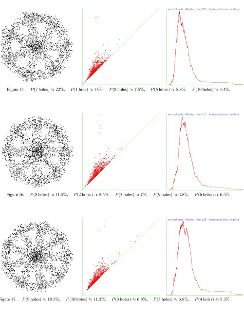
The left hand side pictures in Fig.15–17contain a cloud
C uniformly generated around wheels (the boundaries of
regular polygons with the radii to all vertices). The mid-dle pictures show the persistence diagramsPD{C↵}. The
right hand side pictures are the staircasesPS{C↵} giving
[image:8.612.310.540.412.515.2] [image:8.612.53.267.534.676.2]Figure 15. P(7 holes)⇡22%, P(1 hole)⇡14%, P(8 holes)⇡7.5%, P(6 holes)⇡5.8%, P(10 holes)⇡4.4%.
Figure 16. P(8 holes)⇡11.5%, P(2 holes)⇡8.5%, P(3 holes)⇡7%, P(9 holes)⇡6.8%, P(6 holes)⇡6.5%.
Figure 18. P(25 holes)⇡8.8%, P(0 holes)⇡5.4%, P(15 holes)⇡5%, P(27 holes)⇡4.6%, P(20 holes)⇡3.5%.
Figure 19. P(36 holes)⇡9.4%, P(31 holes)⇡4.8%, P(33 holes)⇡4.8%, P(2 holes)⇡4.6%, P(1 hole)⇡3.2%.
[image:10.612.65.553.518.686.2]