Efficacy of a GPGPU Acceleration to Inundation Flow Simulation in Tonle Sap Lake in Cambodia

Efficacy of a GPGPU-Acceleration to Inundation

Flow Simulation in Tonle Sap Lake in Cambodia

Takashi Nakamura1,*_{, Shun Murakami}2_{, Lun Sambo}3_{, and Hideto Fujii}4

1Department of Global Engineering for Development, Environment and Society, Tokyo Institute of Technology, 4259 Nagatsuta, Midori-ku, Yokohama 226-8502, Japan

2IDAJ Co., LTD., 2-2-1-1 Minato Mirai, Nishi-ku, Yokohama 220-8137, Japan

3Department of Rural Engineering, Institute of Technology of Cambodia, PO Box 86, Russian Federation Blvd., Phnom Penh, Cambodia

4Department of Food, Life and Environmental Sciences, Yamagata University, 1-23 Wakaba-machi, Tsuruoka, Yamagata 997-8555, Japan

E-mail: *_{[email protected] (Corresponding author)}

Abstract. A new two-dimensional numerical model is developed for a rapid computation of the sea-sonal inundation phenomena in Tonle Sap Lake in Cambodia. In order to overcome a huge computa-tional cost for a prolonged analysis over an extensive area, the General-Purpose computing on Graphics Processing Units (GPGPU) technology is applied to the model. The developed model is applied to a solution of seasonal inundation process for the 154 days in 2002. Calculated result is compared with observational data and satellite remote sensing. It is found that the developed model seems to success-fully reproduce reasonable progress/regress of inundation. A breakdown of the total elapsed time for the numerical analysis is considered in a detail. It is found that the GPGPU technology can accelerate the solution more than one hundred times faster by employing a simple rectangular mesh and coding to reduce a memory access overhead.

Keywords:GPGPU, numerical inundation flow model, shallow water equation, Tonle Sap Lake.

ENGINEERING JOURNALVolume 23 Issue 1

1. Introduction

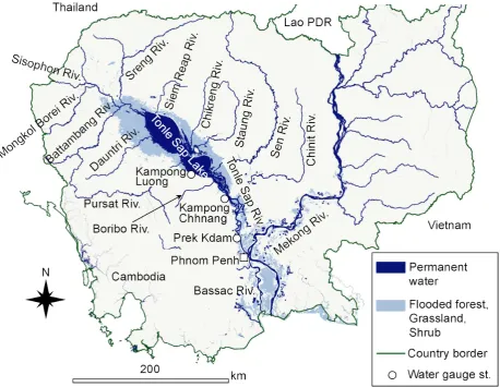
Tonle Sap Lake (TSL) is the largest freshwater lake on Southeast Asia. The lake is located roughly at the center of the kingdom of Cambodia (Fig. 1). Through Tonle Sap River (TSR) located on the southeast of the lake, TSL is connected to the Mekong River (MR). TSL has a quite unique hydraulic and hydrological characteristic. The climate of the region is characterized by clearly divided dry (from November to April) and wet (from May to October) seasons [1]. During the dry season, TSL releases water to the MR (maximum discharge 10,000 m3_{/s) and its depth is kept to be shallow (minimum} monthly depth is 1.5 m) [2, 3]. Conversely, during the wet season, TSL receives a large amount of water from the MR due to reversal flow caused in TSR [4]. The maximum flux of the reversal flow can reach up to about 10,000 m3_{/s. This phenomenon causes a significant rising of TSL’s water level and} fills up wide floodplains surrounding the lake. At the end of wet season, the lake’s depth reaches up to 10 m and surface water area expands to six-fold area (15,000 km2_{) compared to that of dry season} (2,600 km2_{) [2]. In addition to a function as a detention reservoir for the Mekong Delta area [3], TSL} is providing important infrastructures of society and ecosystem. TSL provides the largest fishery in Cambodia, which accounts for 70%of the protein consumed in the country [5]. The flooded forest, shrub, grassland and agricultural field on the floodplain provide habitats and foods for a wide range of species including globally threatened species. The lake and its floodplain support the productive biodiversity.

The recent researches suggest that the ecosystem of TSL had achieved a certain stage of maturity until at least 2010 and its food web is being a vulnerable, albeit with the relatively healthy ecosystem [6, 7]. Furthermore, the future of TSL is uncertain. TSL and the MR basins are changing at a rapid rate under the severe pressures such as economic growth, population increase, infrastructure development and climate change [2, 8]. Recently, the Mekong River Commission (MRC) investigated eight different future scenarios in which probable development of water infrastructures and climate change were considered [8]. The study concluded that a flooded depth during wet season could be reduced by 0.5 m. This change could threaten the highly productive biodiversity in TSL by reducing the flooded area by 400-900 km2_. These findings suggest that TSL is now standing at a turning point for sustaining its brilliant ecosystem and valuable resources.

In order to keep using the TSL’s resources sustainably in assessing environmental and ecological risks, well understanding of the hydraulics is needed. Nonetheless, at the present time, the hydraulic re-search on TSL still remains at an early stage. Indeed, while surface hydrology of TSL is well understood and has been explained through many numerical models [9, 10, 11, 12, 13], a few numerical hydraulic dynamics models have been successfully applied to analysis of a whole area of TSL [11, 12, 13]. There is no doubt that one of the barriers to apply the hydraulic model is a huge computational cost requested by topographical and hydraulic features of TSL. Namely, long-term and large-scale computations should be needed for the practical assessments because the TSL’s water bodies spreads over a quite wide area (almost 200×75 km2 _{in wet season) and important environmental phenomena are caused by the} sea-sonal change of hydraulic conditions such as the reversal flow during wet season. To overcome the huge computational cost, in the case of WUP-JICA model [11], TSL is represented as a network of one-dimensional channels and two-one-dimensional progress of inundation is approximately solved by the rapid one-dimensional solutions. Even in the case of the MRCS/WUP-FIN model [12], while the model is a multi-dimensional flow model that does not use the approximation with the one-dimensional channels, it is recommended that the spatial size of computational mesh should be larger than 1 km to finish the computation with affordable elapsed time [13]. On the other hand, recently it has been known that the minute fluctuation of altitude over the floodplain can affect to the inundation flow [8]. Thus, in order to advance the practical assessments of TSL in the future, the model is being demanded to employ the finer mesh and cope with much more computational cost than the past.

Fig. 1. Major river system in Cambodia.

Processing Unit (GPU), which is originally designed to create images for output to a display device. The GPGPU technology has already been applied to inundation flow analysis. However, because the past applications mainly targeted tsunami propagation in a short-term period and inundation in relatively small area along a river [16, 17], there is no knowledge of applicability to a long-term and large-scale sim-ulation of the seasonal flooding in TSL. Thus, in this study, we developed a new inundation flow model with the GPGPU and investigated the efficacy of a GPGPU-acceleration to the inundation analysis of TSL.

In the model development, we paid much attention to serviceableness for the daily management of the lake. This study is conducted as a part of the international research project, “Establishment of Envi-ronmental Conservation Platform of Tonle Sap Lake” supported by Science and Technology Research Partnership for Sustainable Development (SATREPS) [18]. The goal of the project is establishment of water-environment analytical tools that help science-based management by the Cambodian government. The present model is expected to take a part in the tools. Due to an aftereffect of unfortunate Cambodia Civil War in the last century, even now the Cambodian technicians with the highly specialized skills of the numerical hydraulic simulation seem to be lack. Therefore, in order to utilize the model for daily assessment, the simulation model should be easy-to-use and easy-to-understand. Consequently, we de-cided that the inundation flow model is developed with the simplest mesh and well-established schemes although there are various inundation models using a sophisticated mesh system and advanced schemes of high-order accuracy [16, 17].

long-term simulation of TSL with a fine mesh-size (250 m). The effectiveness of the present model is discussed by comparing the elapsed time with a conventional model, which does not use the GPGPU solution.

2. Numerical Model

2.1. Governing Equation

The model solves the two-dimensional shallow water equation in a Cartesian coordinates(x, y);

∂tw+∂xF(w) +∂yG(w) =Sbtm+Sf ric+SCor+SRey, (1)

w= (h, hu, hv)T,F(w) = (hu, hu2+gh2/2, huv)T,G(w) = (hv, huv, hv2+gh2/2)T, (2)

whereh(t, x, y)is depth,u(t, x, y)andv(t, x, y)are depth-averaged velocity in thexandydirections, respectively, w is a vector of Riemann invariants to be solved, F and G are the tensor fluxes. The symbol∂λarepresents a partial differential operation∂a/∂λ.Sbtm,Sf ric,SCorandSReyrepresent the forces due to the spatial gradient of water level, bottom friction, Coriolis effect and Reynolds stress, respectively [19];

Sbtm = gh(0, ∂xz, ∂yz)T, (3)

Sf ric = −g(n∗)2h−1/3(0, u(u2+v2)1/2, v(u2+v2)1/2)T, (4)

SCor = fch(0, v,−u)T, (5)

SRey = (0, ∂x(νth∂xu) +∂y(νth∂yu), ∂x(νth∂xv) +∂y(νth∂yv))T, (6)

wherez(x, y)is an altitude of bed surface,n∗Manning’s roughness coefficient andfcCoriolis coefficient. In this work, a linear eddy viscosity model is employed as the Reynolds stress. The turbulent viscosity coefficientνtis assumed to be constant that is calculated from a computational mesh sizeLby using the Richardson’s 4/3 power law;νt= 0.01L4/3[20, 21].

2.2. Mesh and Discretization

Equation (1) is solved with a finite volume method [22]. In order to make the model to-use and easy-to-understand, a uniform rectangular mesh system and the simple 1st-oder Roe approximate Riemann scheme [23] are employed. The variablewis stored at the centroids of each computational cell (Fig. 2). By dividing the time domain in sub-interval[tn, tn+1]with time increment∆t, Eq. (1) is discretized using the finite volume approach;

wn_ij+1=wn_ij+∆t ∆x

( F_i−1

2,j−Fi+ 1 2,j ) +∆t ∆y ( G_i,j−1

2 −Gi,j+ 1 2

)

+ ∆t

∆x∆y

∫ y_{j+ 1}

2

y_j−1 2

∫ x_{i+ 1}

2

x_i−1 2

Sdxdy, (7)

where w_ijn represents the averaged value of win the cell(xi, yj)at timetn and S = Sbtm +Sf ric+ SCor+SRey. Fi±₂1,j =F(wni±1

2,j

)andG_i,j±1

2 =G(w

n i,j±1

2

Fig. 2. Computational mesh system.

(a) Before wetting (b) After wetting

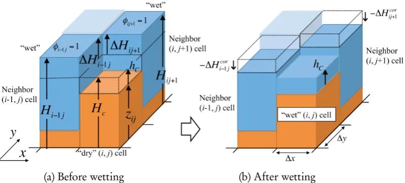
Fig. 3. Schematic view of wetting process. For simplicity, only two neighbour cells(i−1, j)and

(i, j+ 1)are shown.

2.3. Wetting and Drying Algorithm

In order to model inundation processes, a simple element removal algorithm is employed [25]. All computational cells are classified into the “wet (flooded) cell where the water body exists” and “dry (no flooded) cell where land surface is not covered with the water”. The “dry cells” are removed from the calculation and the shallow water equation (1) is solved only at the “wet cells”. To trace a temporal change of inundation area, the classification is updated every time step and the newly wetting/drying cells are detected by checking the water depth after solving Eq. (7). If water depth in a “wet cell” becomes shallower than a certain small threshold value hc, all water body is considered to migrate from the cell and the cell is changed from “wet” to “dry”. The change from “dry” to “wet” is detected by comparing the water level. Let us consider a “dry” (i, j) cell with its neighbor four “wet” cells,

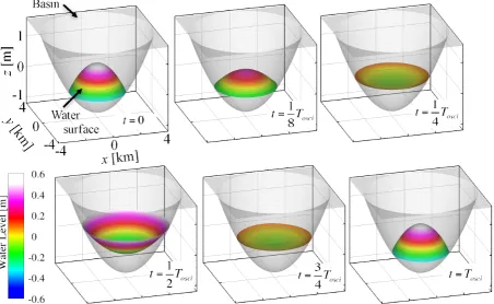
Fig. 4. Water surface calculated for two-dimensional sloshing problem.

calculated as

Ve=ϕi−1j∆Hi−1j +ϕi+1j∆Hi+1j+ϕij−1∆Hij−1+ϕij+1∆Hij+1, (8)

∆Hlm =Hlm−Hc, ϕlm= {

∆x∆y if (l, m) cell is wet

0 if (l, m) cell is dry . (9)

Then, if the excess water volumeVeis enough large to fill in the “dry”(i, j)cell with ahcthick water layer (Ve > ∆x∆yhc), a portion ofVe in the neighbor cells is considered to flow into the “dry”(i, j) cell and the(i, j)cell is changed to “wet” cell which has the minimum water depthhij =hc(Fig. 3(b)). In that case, the water level at the neighbor “wet”(l, m)cells is reduced by∆H_lmcor =hc(ϕlm∆Hlm/Ve) in order to cancel the increasing of water volume due to the newly “wetting”(i, j)cell.

2.4. Two-Dimensional Sloshing Benchmark Problem

To check the fundamental accuracy of the model, the present model is applied to a two-dimensional sloshing problem in an elliptic paraboloid basin. For the problem, Thacker derived a theoretical solution given by the elliptic paraboloidal water surface that oscillates with a constant periodTosci[26]. In the test problem, we assumed the same initial conditions as Thacker used. Initially, a stationary water body locally stands within aL = 2km radius of the bottom of the basin. A profile of the water surface is given by a rotating circular wave whose wave height∆ ˜His 1 m. The calculations is conducted for one recurrence periodTosci= 1774sec. The time increment∆tis determined at each time step in order to keep the CFL number for the water surface wave less than 0.1 (roughly∆t∼0.2sec). ∆x = ∆y = 8

Fig. 5. Cross-sectional water surface profile calculated for two-dimensional sloshing problem [Cross-section along the centerliney= 0(red) and diagonal liney=x(blue)].

As shown in Fig. 5, through the computation, the maximum difference between the calculated water level and exact solution is less than2.0cm, and the calculated result agrees very well with the theoretical solution.

3. Acceleration by GPGPU

3.1. GPU Architecture

Fig. 6. GPU expansion card in PC.

Fig. 7. Schematic view of GPU architecture (NVIDIA Tesla P100).

access speed to the shared memory from the CUDA cores is very fast. On the other hand, “Global memory” is an off-chip memory allocated in DRAM chips on the expansion card. In contrast to the shared memory, while the access speed to global memory is slower than that to shared memory, its large capacity can reach up to several gigabytes and all CUDA cores are allowed to access to it.

3.2. Basic Concept of GPGPU-Acceleration of the two-dimensional Shallow Water Equation

Acceleration by the GPGPU is based on a parallel computing using the massive CUDA cores. The NVIDIA provides a programing platform called “CUDA” for the GPGPU parallel computing [14]. This CUDA platform consists of a compiler and programing libraries designed to work with C, C++ and Fortran languages. By using its API functions, we can relatively easily develop a GPGPU-accelerated parallel code without a troublesome programing to control the GPU device.

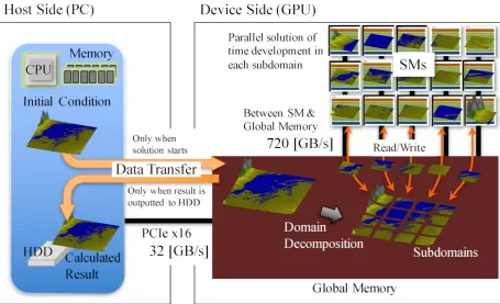
side”. Then, the solution starts on the GPU. On the device side, by a repeated calculation of Eq. (7) with the wetting/drying treatments, time development of the water depth and water current is solved. In order to accelerate this calculation, we employed a parallel computing based on a domain-decomposition approach. A whole computational domain is split into many “subdomains”, which are small rectangular areas containing the same number of computational cells. In this work, a size of each subdomain is set to 32_×32 cells. The SMs in the GPU are assigned to the subdomains one by one, and each SM is charged to solve the new value w_ijn in the assigned subdomain. This calculation can be conducted simultaneously with the other SMs because all calculations in the present model are based on the simple explicit formulation. In addition to this parallelizing by the domain-decomposition, simultaneously, the solution in each subdomain can be also parallelized by using 64 CUDA cores grouped in each SM.

Even if the CUDA platform is used, various contrivances are needed in order to archive a satisfactory acceleration [14, 15]. One of the most important contrivances is reducing a memory access overhead because memory access latency is several tens or hundreds times larger than that of basic arithmetic operations calculated by the CUDA core. In the present model, while all data transfers in the device side are generally coded to be coalescing memory access without bank conflicts in order to reduce the latency, the calculation in a CUDA core is coded to use the shared memory as a data buffer in order to reduce the number of times that the core reads data from the global memory. While data transfer between the device and host sides is conducted by the PCI Express (PCIe) bus which connects the expansion GPU card with PC, speed of the bus (32GB/s) is generally quite slow even in comparison with the slowest data transfer within the device side (720GB/s between the global memory and CUDA cores). Thus, the present model is coded in order to reduce the frequency of these quite slow data transfer to the minimum; normally any data is not transferred between the host and the device after translating the initial conditions except when the calculated results are outputted to a HDD at certain time intervals.

(a) (b)

Fig. 9. Computational Domain; (a) topographic map of a whole domain and (b) birds-eye view of a part area given by a white dashed box in panel (a).

Table 1. Specification of processers used for computation.

Clock Used Memory Transfer Peak Speed [GFLOPS]† Processer Name [GHz] Cores Bandwidth[GB/s] (Normalized by CPU)

CPU: Intel Xeon E5-2630 v4 2.2 1 68.3 28.8 (1)

GPU: NVIDIA Tesla P100 1.328 3584 732 4700 (163)

†:performance for double precision data format.

4. Application to the Tonle Sap Lake

The developed model is applied to an inundation simulation in TSL. The calculated results are com-pared to the observed data and satellite remote sensing. Efficacy of GPGPU-acceleration is checked by comparison with a conventional model that uses only the CPU.

4.1. Computational Conditions

Fig. 10. Hydraulic conditions during the calculated period.

fortnightly ADCP data, is imposed as a boundary condition at the downstream end of TSR, where a red line named “PK BC” is shown in Fig. 9 (a). Together with the flow rate, an observational time series data of water level at Prek Kdam is imposed at the same boundary. For the eleven major tributaries except the Boribo River, time series data of flow rate provided by MRC [30] is imposed as a boundary condition at each position represented by a red box in Fig. 9 (a). The top four flow rate in the tributaries are shown in Fig. 10 (c) and (d). On the other hand, the boundary condition is not imposed on the Boribo River, for which the observational data is unavailable. Because the small basin area of the Boribo River (827 km2_{) accounts only for 1.4%of the total area of the TSL (57,632 km}2_{), it is expected that the} disregard of the Boribo does not have a large influence on the calculated result. Time increment is set to∆t = 10sec. As initial conditions, while stationary water body (u = v = 0) is assumed, a spatial profile of water level is set by a linear-interpolation with the observed water level at three water gauge stations, Prek Kdam, Kampong Chhnang and Kampong Luong.

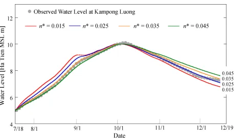
be a dominant factor to affect a calculated result of water level. Therefore, we conducted a series of simulations with differentn∗ raging from 0.015 m−1/3_{sec (normal value for an earthen water channel} without vegetation) to 0.045 m−1/3_{sec (for a floodplains with scattered bush and heavy weeds). Then,} we determined the most proper value by comparing the simulations.

The GPU and CPU used in this work are shown in Table 1. The double precision format is used for all of real numbers in the calculation. Speed of calculation by a possessor is usually measured in FLOPS, which stands how many times the possessor can perform arithmetical operations with floating-point data during one second. Theoretically expected peak speed of the GPU reaches up to 4,700 GFLOPS, which is 163 times faster than that of the CPU (28.8 GFLOPS).

Fig. 11. Influence of Manning’s roughness coefficientn∗on the water level at Kampong Luong. Cir-cles and solid lines represent observational data and calculated results, respectively.

Table 2. Nash–Sutcliffe model efficiency coefficient for the solution of water level.

Manning’s roughness coefficientn∗[m−13sec] NSE

0.015 0.924

0.020 0.974

0.025 0.979

0.030 0.989

0.035 0.990

0.040 0.982

Fig. 12. Calculated inundation area and water level (n∗= 0.035).

4.2. Calculated Results

Figure 11 shows a dependency of calculated water level on Manning’s roughness coefficient n∗. As shown in Fig. 10 (b), before the beginning of Oct., water flows from Tonle Sap River to Tonle Sap Lake due to the reversal flow. Therefore, the observational water levels at Kampong Luong and Kampong Chhnang continuously rise until the beginning of Oct. After water level reaches to the peak at the beginning of Oct., water level starts to fall because a direction of flow in Tonle Sap River changes to the normal flow. As shown in Fig. 11, before the beginning of Oct., calculated water level rises more rapidly asn∗ decreases. Similarly, after the beginning of Oct, the calculated fall of water level becomes to be more rapid asn∗decreases. Such acceleration of the change of water level is reasonable from a viewpoint of physical meaning ofn∗. Because the frictional forceSf ricis proportion to(n∗)2as shown in Eq. (4), frictional resistance to the water flow becomes to be weaker asn∗decreases. Therefore, transportation of water to/from TSL is enhanced and the change of water level is accelerated by decreasingn∗. Table 2 shows the Nash–Sutcliffe model efficiency coefficient (NSE) estimated by

NSE= 1− 1 N s2

N ∑

n=1

(H_Obsn −H_Simn )2, (10)

whereN is the number of observational data. Hn

Obs andHSimn are observational and calculated water levels, respectively. s2 is the sample variance ofH_Obsn . NSE indicates the relative magnitude of the model’s prediction error compared to the observed data variance. “NSE=1” means that the calculated result exactly agrees with the observed data [4]. As shown in Table 2, NSE reaches a peak atn∗= 0.035

m−13sec. The maximum value (NSE=0.990), which is close to 1, means that the present model has a

Fig. 13. Comparison of calculated water level with observational data (n∗ = 0.035).

the calculated results with the value are shown in the following.

Figure 12 shows the temporal change of calculated inundation area and water level. While the el-evation in the non-flooded area is represented in monochrome, the water level in the flooded area is shown in a color contour map. As shown in Fig. 10(a), the highest water level was observed around the beginning of Oct. when the reversal flow ended. As shown in Fig. 12, the present model reproduces not only this rising of water level and the expanding of inundation area, but also the shrinking process of flooded after the beginning of October.

Figure 13 shows a comparison with the water level observed at two water gauge stations, Kampong Luong and Kampong Chhnang. The Kampong Luong and Kampong Chhnang locate on TSL and TSR, respectively and the distance between the two stations reaches to about 70 km (Fig. 9). As shown in Fig. 13, the calculated water levels agree well with the observational data. Furthermore, the present model successfully reproduces the time lag in rising of water level between the two water gauge stations during the period before the water level reaches to the peak at the beginning of Oct. On the other hand, during the later period from Oct. to Dec. in that the water level falls, calculated water level slightly differs from the observation while the difference is kept to be no more than 20 cm. Although the concrete cause of the degradation of results has not been specified at the present time, there are some suspect causes; low temporal resolution of observed data used for the boundary conditions (especially, fortnightly data of flow rate at Prek Kdam), disregard for the precipitation/evaporation processes and employment of uniform Manning’s roughness coefficient for the whole area without regard to spatial change of land cover. It is expected that the model performance can be further improved by coping the above suspect causes.

Figure 14 shows a comparison of inundation area to the satellite remote sensing. In each panel, while the white lines show the water’s edge calculated by the present model, the red pixels represent the water existence area detected by the Normalized Difference Water Index (NDWI) [33]. The NDWI is estimated with Landsat-7 ETM+ data:

NDWI= (VIS−SWIR)/(VIS+SWIR), (11)

Fig. 14. Comparison of inundation area to satellite remote sensing (n∗ = 0.035).

work, band-1 and band-5 of ETM+ are used for the VIS and SWIR respectively, and NDWI = 0.4 is used for the threshold value of water existence. While the calculated inundation area seem to be different from the remote sensing in the northwest part where the water cannot be detected by the satellite remote sensing due to the flooded forest covering the water surface, it is found that the calculated inundation area agrees with the remote sensing results as a whole.

4.3. Efficacy of the GPGPU-Acceleration

The present parallel computing model with the GPU is recoded into a conventional non-parallel com-puting model, which uses only the CPU without the GPU. In order to assess the efficacy and usability of GPGPU acceleration, elapsed time for the simulation of TSL is compared between the present model and the conventional model. The conventional model is not implemented in a parallel computing model and only one core on the CPU is used for the simulation. Table 3 shows the elapsed time spent on the solution of the 154 days in TSL. As shown in column (a), while the conventional model spends almost one week, the present model enables to finish the solution in an hour and a half. This fact means that even a yearlong simulation can be finished in less than four hours by the present model. The speed of the present model, which can be estimated from the inverse of the total elapsed time, reaches up to 104 times faster than that of the conventional model. While this acceleration of the speed is surprising, the measured speed of the present model degrades from the theoretically expected peak speed of the GPU that is 163 times faster than the CPU (see Table 1).

cannot be accelerated at all because the reading/writing to the disk drive is essentially a sequential process and the process cannot be carried out in parallel. Therefore, while time for the calculation is sub-second (column (a) of Table 4), time for the data output reaches up to a few seconds for both the conventional model and present model (column (c) of Table 4). Generally speaking, the overhead concerning the data output tends to be a dominant factor for the effective GPGPU acceleration, because the overhead of output becomes to be relatively longer than the time for the calculation that can be drastically shortened by the parallel computing of the GPGPU. Actually, as shown in the breakdown of the total elapsed time (column (b) and (c) of Table 3), the data output accounts for 36%of the total elapsed time in the present model and this large overhead causes the degradation of the computing speed from the theoretically expected value.

It must be valuable to point out that the data transfer process is also important factor in the GPGPU computing to archive a rapid solution as well as the output process. The column (b) of Table 4 shows time spent to transfer the calculated data from the “device side” (GPU) to the “host side” (CPU) before outputting the data to a HDD. Because of slow transfer via the PCIe bus, in the present model, the time of the transferring (12 msec; column (b) of Table 4) becomes to be almost five times longer than that of calculation (2.5 msec; column (a) of Table 4). This fact suggests that the frequency of data transfer between the “device” and “host” must be reduced to minimum in order to get the effective GPGPU acceleration as it was done in the present model.

Table 3. Elapsed time for the solution of the TSL.

(a) Total (b) For calculation (c) For data output† (Normalized speed) (%in the total) (%in the total) Conventional model 6.34 day (1) 6.32 day (99.7%) 31.8 min ( 0.3%) Present model 86.8 min (104) 55.2 min (63.6%) 31.6 min (36.4%)

†:interim results are outputted every 6 hours (every 2160 time steps)

Table 4. Time consumed to carry out each process once.

(a) Calculation for one time step (b) Data transfer (c) Data output (Normalized speed) from GPU to PC to HDD

Conventional model 0.41 sec (1) - 3.1 sec

Present model 2.5 msec (165) 12 msec 3.1 sec

5. Conclusions

Toward establishment of a hydraulic simulation model for daily management of TSL, a new GPGPU-accelerated two-dimensional inundation flow model is developed and efficacy of the model is investi-gated. The developed model is applied to TSL and the inundation process for the 154 days in 2002 is reproduced. The following conclusions are drawn based on the application.

• While the accuracy of the present model has not been fully verified because of the lack of ob-served hydraulic data, by comparing with the obob-served data of water level and satellite remote sensing analysis, it is found that the present model seems to successfully reproduce the reasonable progress/regress of inundation in TSL.

• The calculation speed of the present model surprisingly reaches to more than one hundred times faster compared to the conventional model. By investing the breakdown of elapsed time, it is confirmed that the reduction of the overhead of data transfer/output becomes to be a crucial point to archive a satisfactory GPGPU-acceleration.

Acknowledgement

Authors thank the Mekong River Commission (MRC), the Tonle Sap Authority and Ministry of Water Resources and the Meteorology Cambodia (MOWRAM) for providing the dataset and kind supports. This research was supported by Science and Technology Research Partnership for Sustainable Devel-opment (SATREPS), Japan Science and Technology Agency (JST)/Japan International Cooperation Agency (JICA).

References

[1] C. Phoeurn and S. Ly, “Assessment of satellite rainfall estimates as a pre-analysis for water environ-ment analytical tools: A case study for Tonle Sap Lake in Cambodia,”Engineering Journal, vol. 22, pp. 229–241, 2018.

[2] M. E. Arias, T. A. Cochrane, T. Piman, M. Kummub, B. S. Caruso, and T. J. Killeen, “Quantifying changes in flooding and habitats in the Tonle Sap Lake (Cambodia) caused by water infrastructure development and climate change in the Mekong Basin,”J. Environ. Manag., vol. 112, pp. 53–66, 2012.

[3] MRC, “Overview of the hydrology of the Mekong Basin,” Mekong River Commission, Vientiane, Lao PDR, Tech. Rep., 2005.

[4] S. Ly, L. Kim, S. Demerre, and S. Heng, “Flood mapping along the lower Mekong River in Cam-bodia,”Engineering Journal, vol. 22, pp. 269–278, 2018.

[5] N. Bonheur and B. D. Lane, “Natural resources management for human security in Cambodia’s Tonle Sap Biosphere Reserve,”Environ. Sci. Pol., vol. 5, pp. 33–41, 2002.

[6] R. Cheaa, C. Guoa, G. Grenouilleta, and S. Lek, “Toward an ecological understanding of a flood-pulse system lake in a tropical ecosystem: Food web structure and ecosystem health,”Ecol. Model., vol. 323, pp. 1–11, 2016.

[7] A. Ohtaka, R. Watanabe, S. Im, R. Chhay, and S. Tsukawaki, “Spatial and seasonal changes of net plankton and zoobenthos in Lake Tonle Sap, Cambodia,”Limnology, vol. 11, pp. 85–94, 2010. [8] MRC, “Impacts on the Tonle Sap ecosystem, Technical note 10, assessment of basin-wide

develop-ment scenarios. In: Basin Developdevelop-ment Plan Programme, Phase 2,” Mekong River Commission, Vientiane, Lao PDR, Tech. Rep., 2010.

[9] M. Kummu, S. Tes, S. Yin, P. Adamson, J. Józsa, J. Koponen, J. Richey, and J. Sarkkula, “Water balance analysis for the Tonle Sap Lake–floodplain system,”Hydrol. Process., vol. 28, pp. 1722–1733, 2014.

[10] H. Inomata and K. Fukami, “Restoration of historical hydrological data of Tonle Sap Lake and its surrounding areas,”Hydrol. Process., vol. 22, pp. 1337–1350, 2008.

[11] WUP-JICA, “The study on hydro-meteorological monitoring for water quantity rules in Mekong river basin (Final Report),” Japan International Cooperation Agency, Tech. Rep., 2004.

[12] MRCS/WUP-FIN, “Modelling Tonle Sap watershed and lake processes for environmental change assessment,” Mekong River Commission, Vientiane, Lao PDR, Tech. Rep., 2003.

[13] MRCS/WUP-FIN, “Hydrological, environmental and socio-economic modelling tools for the lower mekong basin impact assessment Technical Paper No. 1,” Mekong River Commission, Vi-entiane, Lao PDR, Tech. Rep., 2008.

[15] D. B. Kirk and W. W. Hwu, Programming massively parallel processors, third edition: a hands-on approach. Morgan Kaufmann, Burlington, USA, 2016.

[16] A. Lacasta, M. Morales-Hernandez, J. Murillo, and P. Garcia-Navarro, “GPU implementation of the 2D shallow water equations for the simulation of rainfall/runoff events,”Environ. Earth Sci., vol. 74, pp. 7295–7305, 2015.

[17] R. Vacondio, A. D. Palub, A. Ferrari, P. Mignosa, F. Aureli, and S. Dazzi, “A non-uniform efficient grid type for GPU-parallel shallow water equations models,”Environ. Modeling Software, vol. 88, pp. 110–137, 2017.

[18] SATREPS, “Establishment of Environmental Conservation Platform of Tonle Sap Lake,” https://sites.google.com/site/satrepscambodia/, [Accessed: Jun, 2017].

[19] Y. Ding, Y. Jia, and S. S. Y. Wang, “Identification of Manning’s roughness coefficients in shallow water flows,”J. Hydr. Eng., vol. 130, pp. 501–510, 2004.

[20] L. F. Richardson, “Atmospheric diffusion shown on a distance-neighbor graph,” Proc. Roy. Soc. London, vol. A110, pp. 709–739, 1926.

[21] H. B. Fischer, E. J. List, R. C. Y. Koh, J. Imberger, and N. H. Brooks,Mixing in inland and coastal waters. Academic Press, New York, 1979.

[22] F. Moukalled, L. Mangani, and M. Darwish, The finite volume method in computational fluid dy-namics. Springer International Publishing, Switzerland, 2015.

[23] P. L. Roe, “Approximate riemann solvers, parameter vectors, and difference schemes,”J. Comput. Phys., vol. 43, pp. 357–372, 1981.

[24] F. Benkhaldoun, I. Elmahi, and M. Seaid, “A new finite volume method for flux-gradient and source-term balancing in shallow water equations,”Comput. Methods Appl. Mech. Engrg., vol. 199, pp. 3324–3335, 2010.

[25] S. C. Medeiros and S. C. Hagen, “Review of wetting and drying algorithms for numerical tidal flow models,”Int. J. Numer. Meth. Fluids, vol. 71, pp. 473–487, 2013.

[26] W. C. Thacker, “Some extent solutions to the nonlinear shallow-water wave equations,” J. Fluid Mech., vol. 107, pp. 499–508, 1981.

[27] A. Jarvis, H. I. Reuter, A. Nelson, and E. Guevara, “Hole-filled SRTM for the globe version 4,” available from the CGIAR-CSI SRTM 90m Database http://srtm.csi.cgiar.org, 2008 [Accessed: Jun, 2017].

[28] Mekong River Commission and Ministry of Public Work and Transport of Cambodia, “Hydro-graphic atlas Mekong River in Cambodia,” Mekong River Commission and Ministry of Public Work and Transport of Cambodia, Tech. Rep., 1999.

[29] H. Fujii, H. Garsdal, P. Ward, M. Ishii, K. Morishita, and T. Boivin, “Hydrological roles of the Cambodian floodplain of the Mekong River,”Intl. J. River Basin Management, vol. 1, pp. 253–266, 2003.

[30] Mekong River Commission, “MRC Data and Information Services Portal,” available from http://portal.mrcmekong.org/index, [Accessed: Jun, 2017].

[31] J. V. Phillips and S. Tadayon, “Selection of Manning’s roughness coefficient for natural and con-structed vegetated and non-vegetated channels, and vegetation maintenance plan guidelines for vegetated channels in central Arizona,” Scientic Investigations Report 2006–5108, U.S. Geological Survey, Tech. Rep., 2006.

[32] V. T. Chow,Open-channel hydraulics. McGraw-Hill Book Co., New York, 1959.

[33] B. Gao, “NDWI-a normalized difference water index for remote sensing of vegetation liquid water from space,”Remote Sensing of Env., vol. 58, pp. 257–266, 1996.

Appendix

the fluxesF,Gand source termsSin Eq. (7). By assuming that Riemann invariantswhas the constant valuewij within each cell, the discretized formulations ofF,GandSare derived as follows;

F_i−1 2,j =

1 2

(

F(wn_ij) +F(wn_i−1,j))+Aabs_i−1 2

(

w_in_−1,j−wn_ij)+Asgn i−1₂Bi−12,

(A-1)

G_i,j−1 2 =

1 2

(

G(wn_ij) +G(w_i,jn ₋₁))+Cabs_j−1 2

(

w_i,jn₋₁−wn_ij)+Csgn_j−1 2

D_j−1

2, (A-2)

1 ∆x∆y

∫ y

j+ 1₂

y_j−1 2

∫ x

i+ 1₂

x_i−1 2

Sdxdy = 1 2

(

S(wn_i−1 2,j

) +S(wn_i+1 2,j ) ) +1 2 (

S(wn_i,j−1 2

) +S(wn_i,j+1 2 )

)

+

( Asgn_i−1

2

S(wn_i−1 2,j

)−Asgn_i+1 2

S(wn_i+1 2,j ) ) + ( Csgn

j−1₂S(w n

i,j−1₂)−C sgn j+1₂S(w

n i,j+1₂)

)

, (A-3)

supplemented with

Aabs_i−1 2

= 1

2c∗



 (−|λλ33| − ||λ2|λ+2|λ)λ2|3λλ32| λ2||λλ22| −| − |λλ33||λ3| 00

v∗(−λ3|λ2|+λ2|λ3| −2c∗|λ1|) v∗(|λ2| − |λ3|) 2c∗|λ1| 

, (A-4)

Asgn_i−1 2

= 1

2c∗



 00 λ2sgn(λsgn(λ22))−−sgn(λλ3sgn(λ3)3) 00

0 v∗(sgn(λ2)−sgn(λ3)) 0 

, (A-5)

B_i−1 2 =−

g 4



 (hn_i−1,j)20−(hn_ij)2 0



, (A-6)

Cabs_j−1 2

= 1

2c∗∗



 u∗∗(−µ3−|µµ23||+µ2µ|2+|µµ32| −|µ32c| ∗∗|µ1|) 2c∗∗0|µ1| u∗∗|µ(|2µ| − |2| − |µ3µ|3|)

(|µ3| − |µ2|)µ3µ2 0 µ2|µ2| −µ3|µ3| 

, (A-7)

Csgn_j−1 2

= 1

2c∗∗



 00 00 u∗∗sgn(µ(sgn(µ2)2−)−sgn(µsgn(µ3)3))

0 0 µ2sgn(µ2)−µ3sgn(µ3) 

, (A-8)

D_j−1 2 =−

g 4



 00

(hn_i,j−1)2−(hn_ij)2



. (A-9)

Theλmandµm represent the characteristic speeds of the Riemann invariants inxandydirections, respectively;λ1 =c∗,λ2 =u∗+c∗, λ3 =u∗−c∗,µ1 = c∗∗,µ2 =v∗∗+c∗∗,µ3 =v∗∗−c∗∗, where

c∗ = (gh∗)1/2 andc∗∗ = (gh∗∗)1/2 are the phase speed of the shallow-water waves. (h∗, u∗, v∗)and

(h∗∗, u∗∗, v∗∗)are the Roe’s averages given by

h∗= 1 2(h

n

ij +hni−1,j), u∗ = √

hn_ijun_ij+√h_in_−1,jun_i−1,j

√

hn_ij+

√

hn_i−1,j

, v∗ =

√

hn_ijv_ijn +√h_in_−1,jvn_i−1,j

√

hn_ij +

√

hn_i−1,j

, (A-10)

h∗∗= 1 2(h

n

ij +hni,j−1), u∗∗= √

hn_ijun_ij+√hn_i,j−1un_i,j−1

√

hn ij+

√

hn i,j−1

, v∗∗=

√

hn_ijv_ijn +√hn_i,j−1v_i,jn₋₁

√

hn ij+

√

hn i,j−1