Predicting the effect of missense mutations on protein function: analysis with Bayesian networks

White Rose Research Online URL for this paper:

http://eprints.whiterose.ac.uk/1931/

Article:

Needham, C.J., Bradford, J.R., Bulpitt, A.J. et al. (2 more authors) (2006) Predicting the

effect of missense mutations on protein function: analysis with Bayesian networks. BMC

Bioinformatics, 7 (405). ISSN 1471-2105

https://doi.org/10.1186/1471-2105-7-405

[email protected] https://eprints.whiterose.ac.uk/ Reuse

See Attached

Takedown

If you consider content in White Rose Research Online to be in breach of UK law, please notify us by

Open Access

Research article

Predicting the effect of missense mutations on protein function:

analysis with Bayesian networks

Chris J Needham*

_{, James R Bradford}

_{, Andrew J Bulpitt}

_{, Matthew A Care}

and David R Westhead

Address: 1_{School of Computing, University of Leeds, Leeds, LS2 9JT, UK and} 2_{Institute of Molecular and Cellular Biology, University of Leeds,} Leeds, LS2 9JT, UK

Email: Chris J Needham* - [email protected]; James R Bradford - [email protected]; Andrew J Bulpitt - [email protected]; Matthew A Care - [email protected]; David R Westhead - [email protected]

* Corresponding author

Abstract

Background: A number of methods that use both protein structural and evolutionary information are available to predict the functional consequences of missense mutations. However, many of these methods break down if either one of the two types of data are missing. Furthermore, there is a lack of rigorous assessment of how important the different factors are to prediction.

Results: Here we use Bayesian networks to predict whether or not a missense mutation will affect the function of the protein. Bayesian networks provide a concise representation for inferring models from data, and are known to generalise well to new data. More importantly, they can handle the noisy, incomplete and uncertain nature of biological data. Our Bayesian network achieved comparable performance with previous machine learning methods. The predictive performance of learned model structures was no better than a naïve Bayes classifier. However, analysis of the posterior distribution of model structures allows biologically meaningful interpretation of relationships between the input variables.

Conclusion: The ability of the Bayesian network to make predictions when only structural or evolutionary data was observed allowed us to conclude that structural information is a significantly better predictor of the functional consequences of a missense mutation than evolutionary information, for the dataset used. Analysis of the posterior distribution of model structures revealed that the top three strongest connections with the class node all involved structural nodes. With this in mind, we derived a simplified Bayesian network that used just these three structural descriptors, with comparable performance to that of an all node network.

Background

An important aspect of the post-genomic era is to under-stand the biological effects of inherited variations between individuals. For instance, a key problem for the pharmaceutical industry is to understand variations in

drug treatment responses among individuals at the molec-ular level. A single nucleotide polymorphism (SNP) is a mutation, such as an insertion, deletion or substitution, observed in the genomic DNA of individuals of the same species. When the SNP results in an amino acid

substitu-Published: 06 September 2006

BMC Bioinformatics 2006, 7:405 doi:10.1186/1471-2105-7-405

Received: 24 May 2006 Accepted: 06 September 2006 This article is available from: http://www.biomedcentral.com/1471-2105/7/405

© 2006 Needham et al; licensee BioMed Central Ltd.

tion in the protein product of the gene, it is called a mis-sense mutation. A mismis-sense mutation can have various phenotypic effects although we restrict ourselves here to the simplified task of predicting whether a missense muta-tion has an effect or no effect on protein funcmuta-tion.

The wealth of SNP data now available [1-4] has prompted a number of studies on the functional consequences of SNPs. For example, Wang and Moult [5] and Ramensky et al. [6] showed that most of the detrimental missense mutations affect protein function indirectly through effects on protein structural stability particularly disrup-tion to the protein hydrophobic core. The evoludisrup-tionary properties of the mutated residue may also be important determinants of its effect on protein function [7-9], since conserved amino acids tend to be functionally important or critical in maintaining structural integrity. A number of groups have developed strategies to predict the effects of missense mutations by using structural or evolutionary information, or a combination of both. Most of these methods claim prediction accuracies of between 70 – 80% although comparison is extremely difficult due to the use of different data sets and criteria for assigning a mutation as having an effect or not. Chasman and Adams [7] pro-posed a probabilistic method, and Krishnan and West-head [10] evaluated decision trees and support vector machines. Herrgard et al. [11] used structural motifs called Fuzzy Functional Forms to predict the effects of amino acid mutations on enzyme catalytic activity. Deleterious human alleles were predicted by Sunyaev et al. [12] using mostly structural information. By contrast, [13] used purely sequence homology data in their SIFT (Sorting Intolerant From Tolerant) algorithm, although adding structural information resulted in significant improve-ments [14]. Subsequent work has compared SIFT to SVMs and random forests [15]. Cai et al. [16] used a Bayesian framework to predict pathogenic SNPs. Verzilli et al. [17] applied a hierarchical Bayesian multivariate adaptive regression spline (hierarchical BMARS) model for binary classification of the functional consequences of SNPs. Within this model, samples from the posterior distribu-tion were used to highlight properties of the mutated res-idue that are most important in predicting its effect on protein function.

All these methods require either structural or evolutionary data to be available for predictions to be possible. How-ever, there are many proteins that lack any detectable sequence homology to known proteins or a solved 3D structure. In these cases, many prediction methods break down. Therefore a method is needed that can combine both structural and evolutionary information but at the same time tolerate the absence of either without manual intervention. With this in mind we have applied Bayesian networks to the problem of predicting the consequences

of a missense mutation on protein function. Bayesian net-works are probabilistic graphical models which provide a neat compact representation for expressing joint probabil-ity distributions and inference. The representation and use of probability theory makes Bayesian networks suitable for learning from incomplete datasets, expressing causal relationships, combining domain knowledge and data, and avoiding over-fitting a model to training data. As such, a host of applications in computational biology (for example, see [18-20]) have used Bayesian networks and Bayesian learning methodologies [21-23]. Our detailed evaluation of Bayesian network performance in this work is likely to be valuable to many groups working with Baye-sian networks and biological data.

Bayesian networks

Our recent primer [24] introduces Bayesian networks to the computational biologist. Briefly, given a set of varia-bles x = {x₁,..., x_N}, which are represented as nodes in the Bayesian network, a set of directed edges representing relationships between nodes can be defined in a graph structure. To allow efficient inference and learning, a directed acyclic graph (DAG) must be formed, which exploits the conditional independence relations between variables. Using this model structure, model parameters θ in the form of conditional probability distributions (CPDs) between the connected variables may be learned. With discrete data, these model parameters take the form of conditional probability tables (CPTs). Throughout this work, we have used the Bayes Net Toolbox for MATLAB (BNT) [25]. The code used to produce the results pre-sented in this paper is available on request from the authors.

Learning from complete data

The Bayesian learning paradigm can be summarised as:

p(x|D) = ∫p(x|θ)p(θ|D)dθ

I.e., the predictive distribution for a new example observa-tion, given a set of training examples D can be calculated by averaging over all possible models θthe likelihood of the example x given the model, multiplied by the likeli-hood of the model given the training data. For a given model structure the model θcan be thought of as the model parameters that encode the conditional probability distributions between variables and their parents in .

Learning from incomplete data

One advantage of using Bayesian networks is that it is pos-sible to learn model parameters from incomplete training data i.e. in cases where variables are missing. To learn from incomplete data, we used the Expectation-Maximisa-tion (EM) algorithm, which estimates missing values by



computing the expected values and updating parameters using these expected values as if they were observed val-ues.

Structure learning

A fully connected network structure captures relationships (dependencies) between all of the variables. A simpler, more compact model may be produced if conditional independencies between variables are learned. To do this, we used the greedy search algorithm from the Matlab-based structure learning package (SLP) [26] with tabular CPDs and uninformative Dirichlet priors (BDeu). The greedy search algorithm starts with a graph with no edges between the nodes, and aims to maximise a score func-tion: either the full Bayesian posterior or the Bayesian Information Criterion (BIC). At each stage, the neigh-bourhood of the current graph (the set of graphs that dif-fer by adding, reversing or deleting an edge) are considered, and the one with the highest score is chosen, until convergence. We use the notation of Heckerman, where h _{is a model structure hypothesis. From Bayes'}

theorem the posterior distribution for network structures p( h_{|D) is proportional to the marginal likelihood of the}

data p(D| h_{). The full Bayesian posterior can be}

calcu-lated [[27], equation 35], or the BIC approximation can be used, which contains a term to describe how well the maximum likelihood model s for structure h predicts

the data D, and a term that punishes model complexity. For a model with d parameters, built from N samples, the BIC score is:

Inference with missing data

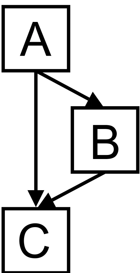
Knowledge of the conditional probability distributions between variables allows us to make predictions about the expected states of variables even if some variables are missing from the test data. For example, if structural infor-mation about a test missense mutation is not available, we can still infer whether the mutation has a functional effect on the protein or not by marginalising over the unknown variables. This is illustrated in a very simple Bayesian network with three nodes, A, B, C, which can take the values {a1,..., }, {b1,..., }, and {c1,...,

} respectively and a structure given by Figure 1. The joint probability over all the variables is:

p(A, B, C) = p(A)p(B|A)p(C|A, B)

Each of the probabilities can be expressed as a conditional probability table in this discrete case. If we wish to infer the value of C given A = a_i and B = b_j then we can calculate the probability of C taking each of the possible values, C = c_k for k = 1,..., N_C by p(c_k|a_i, b_j) read from CPTs. If we wish to infer the value of C given only the value of A, we can marginalise over the unknown variables (in this case, B). Thus:



 

ˆ

θ 

ln ( |p D h)≈ln ( |p D θ_s,h)−dlnN 2

a_NA b_NB

c_NC

Example 3 node Bayesian network

Figure 1

Example 3 node Bayesian network. Example 3 node Bayesian network.

A

B

Results and discussion

The systematic unbiased mutagenesis dataset of lac repres-sor [28,29] and T4 lysozyme [30,31] were used to train and validate the Bayesian networks. Classification of 'effect' and 'no effect' mutations was based on that of [17] in which only those mutations resulting in a significant loss of function were considered 'effect' mutations. As a result, our lac repressor dataset consisted of 823 effect and 2422 no effect mutations, and our T4 lysozyme dataset contained 312 effect and 1320 no effect mutations.

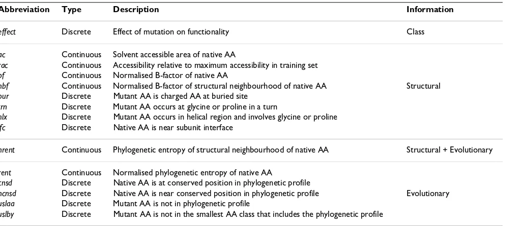
A total of fourteen variables were used to predict whether or not a missense mutation affects protein function (Table 1; Note also the abbreviations introduced – taken from the dataset of [17]). All these variables have been impli-cated in previous studies as useful in discriminating 'effect' from 'no effect' mutations. Six of the variables are continuous (ac, rac, rent, nrent, bf, and nbf), the rest are dis-crete binary. The variables (excluding the class node) can also be sorted into three groups based on the type of bio-logical information they give: structural, evolutionary, or in the case of nrent structural and evolutionary informa-tion.

We used two basic types of Bayesian network structure in this study: naïve and learned. In the naïve structure, the effect node is a parent to all the other nodes in the network structure. Details of the learned structure are provided later. On each of these structures we performed seven experiments:

• all:all: 15 node network trained and tested using all 14 variables listed in Table 1.

• all: noS: 15 node network trained on all variables, tested with evolutionary information only (ac, rac, bf, nbf, bur, trn, hlx, ifc, nrent nodes hidden).

• noS:noS: 6 node network (structural nodes missing) trained and tested with evolutionary information only.

• all:noE: 15 node network trained on all variables, tested with structural information only (nrent, rent, cnsd, ncnsd, uslaa, uslby nodes hidden).

• noE:noE: 9 node network (evolutionary nodes missing) trained and tested with structural information only.

• all:key: 15 node network trained on all variables, tested using three key variables (ac, bur, bf). These key variables were identified by analysing a number of learned struc-tures.

• key:key: 4 node network trained and tested using key var-iables only.

Results of these experiments are presented in Tables 2 and 3. We carried out both homogeneous and heterogeneous cross-validation tests. Homogeneous cross-validation was performed on both lysozyme and lac repressor datasets separately, and a mixed set in which the two datasets were pooled. In each case, data were randomised and divided into 10 equal parts. One part was used as the test set and the remainder as the training set. This procedure was repeated 10 times so that each example (here it is each

p c_k a_i p b_j a p c_{i k} a b_{i j}

b B_j

( | )= ( | ) ( | , )

∈

∑

Table 1: Attributes used for predicting functional effects of missense mutations

Abbreviation Type Description Information

effect Discrete Effect of mutation on functionality Class

ac Continuous Solvent accessible area of native AA

rac Continuous Accessibility relative to maximum accessibility in training set bf Continuous Normalised B-factor of native AA

nbf Continuous Normalised B-factor of structural neighbourhood of native AA Structural bur Discrete Mutant AA is charged AA at buried site

trn Discrete Mutant AA occurs at glycine or proline in a turn

hlx Discrete Mutant AA occurs in helical region and involves glycine or proline ifc Discrete Native AA is near subunit interface

nrent Continuous Phylogenetic entropy of structural neighbourhood of native AA Structural + Evolutionary

rent Continuous Normalised phylogenetic entropy of native AA

cnsd Discrete Native AA is at conserved position in phylogenetic profile

ncnsd Discrete Native AA is near conserved position in phylogenetic profile Evolutionary

uslaa Discrete Mutant AA is not in phylogenetic profile

mutation) was used exactly once for testing. The mean and standard deviation of the ten results were then calcu-lated. In heterogeneous cross-validation, the data set of one protein (e.g. lac repressor) was used as the training set and that of the other protein (e.g. lysozyme) was used as the test set.

Naïve Bayes classifier

all:all

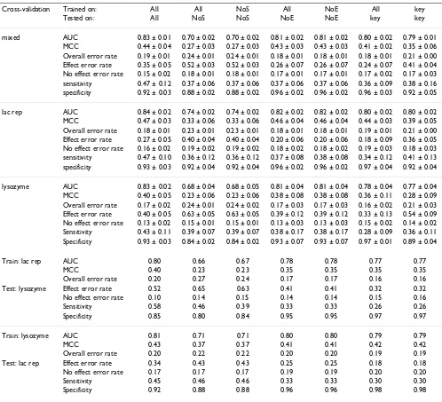
As expected, overall error rates of less than 20% were achieved in all cross validation tests with the all:all model

(Table 2, column 1). These results are consistent with pre-vious studies reporting accuracies of 70 – 80% on similar datasets using similar variables [7,10,17]. Furthermore, all AUC values (Area under ROC curve – see Evaluation measures in Methods section for details of all perform-ance metrics), including those from heterogeneous cross validation were at least 0.80 indicating a robust classifier despite the naïvety of the network structure. We therefore used results on the all:all model as a benchmark for the six other experiments.

Table 2: Results with a naïve Bayes classifier.

Cross-validation Trained on: All All NoS All NoE All key

Tested on: All NoS NoS NoE NoE key key

mixed AUC 0.83 ± 0.01 0.70 ± 0.02 0.70 ± 0.02 0.81 ± 0.02 0.81 ± 0.02 0.80 ± 0.02 0.79 ± 0.01 MCC 0.44 ± 0.04 0.27 ± 0.03 0.27 ± 0.03 0.43 ± 0.03 0.43 ± 0.03 0.41 ± 0.02 0.35 ± 0.06 Overall error rate 0.19 ± 0.01 0.24 ± 0.01 0.24 ± 0.01 0.18 ± 0.01 0.18 ± 0.01 0.18 ± 0.01 0.21 ± 0.00 Effect error rate 0.35 ± 0.05 0.52 ± 0.03 0.52 ± 0.03 0.26 ± 0.07 0.26 ± 0.07 0.24 ± 0.07 0.41 ± 0.04 No effect error rate 0.15 ± 0.02 0.18 ± 0.01 0.18 ± 0.01 0.17 ± 0.01 0.17 ± 0.01 0.17 ± 0.02 0.17 ± 0.03 sensitivity 0.47 ± 0.12 0.37 ± 0.06 0.37 ± 0.06 0.37 ± 0.06 0.37 ± 0.06 0.36 ± 0.09 0.38 ± 0.16 specificity 0.92 ± 0.03 0.88 ± 0.02 0.88 ± 0.02 0.96 ± 0.02 0.96 ± 0.02 0.96 ± 0.03 0.92 ± 0.05

lac rep AUC 0.84 ± 0.02 0.74 ± 0.02 0.74 ± 0.02 0.82 ± 0.02 0.82 ± 0.02 0.80 ± 0.02 0.80 ± 0.02 MCC 0.47 ± 0.03 0.33 ± 0.06 0.33 ± 0.06 0.46 ± 0.04 0.46 ± 0.04 0.44 ± 0.03 0.39 ± 0.05 Overall error rate 0.18 ± 0.01 0.23 ± 0.01 0.23 ± 0.01 0.18 ± 0.01 0.18 ± 0.01 0.19 ± 0.01 0.21 ± 0.00 Effect error rate 0.27 ± 0.05 0.40 ± 0.04 0.40 ± 0.04 0.20 ± 0.06 0.20 ± 0.06 0.18 ± 0.09 0.36 ± 0.05 No effect error rate 0.16 ± 0.02 0.19 ± 0.02 0.19 ± 0.02 0.18 ± 0.02 0.18 ± 0.02 0.19 ± 0.03 0.18 ± 0.03 sensitivity 0.47 ± 0.10 0.36 ± 0.12 0.36 ± 0.12 0.37 ± 0.08 0.38 ± 0.08 0.34 ± 0.12 0.41 ± 0.13 specificity 0.93 ± 0.03 0.92 ± 0.04 0.92 ± 0.04 0.96 ± 0.02 0.96 ± 0.02 0.97 ± 0.04 0.92 ± 0.04

lysozyme AUC 0.83 ± 0.02 0.68 ± 0.04 0.68 ± 0.05 0.81 ± 0.04 0.81 ± 0.04 0.78 ± 0.04 0.77 ± 0.04 MCC 0.40 ± 0.05 0.23 ± 0.06 0.23 ± 0.06 0.38 ± 0.08 0.38 ± 0.08 0.36 ± 0.11 0.28 ± 0.09 Overall error rate 0.17 ± 0.02 0.24 ± 0.01 0.24 ± 0.02 0.17 ± 0.03 0.17 ± 0.03 0.16 ± 0.02 0.21 ± 0.03 Effect error rate 0.40 ± 0.05 0.63 ± 0.05 0.63 ± 0.05 0.39 ± 0.12 0.39 ± 0.12 0.33 ± 0.13 0.54 ± 0.09 No effect error rate 0.13 ± 0.02 0.15 ± 0.01 0.15 ± 0.01 0.13 ± 0.03 0.13 ± 0.03 0.15 ± 0.02 0.14 ± 0.02 Sensitivity 0.43 ± 0.11 0.39 ± 0.07 0.39 ± 0.07 0.38 ± 0.17 0.38 ± 0.17 0.28 ± 0.09 0.36 ± 0.11 Specificity 0.93 ± 0.03 0.84 ± 0.02 0.84 ± 0.02 0.93 ± 0.07 0.93 ± 0.07 0.97 ± 0.01 0.89 ± 0.04

Train: lac rep AUC 0.80 0.66 0.67 0.78 0.78 0.77 0.77

MCC 0.40 0.23 0.23 0.35 0.35 0.35 0.35

Overall error rate 0.20 0.27 0.24 0.17 0.17 0.16 0.16 Test: lysozyme Effect error rate 0.52 0.65 0.63 0.41 0.41 0.32 0.32 No effect error rate 0.10 0.14 0.15 0.14 0.14 0.15 0.16

Sensitivity 0.58 0.46 0.39 0.33 0.33 0.26 0.26

Specificity 0.85 0.80 0.84 0.95 0.95 0.97 0.97

Train: lysozyme AUC 0.81 0.71 0.71 0.80 0.80 0.79 0.79

MCC 0.43 0.37 0.37 0.41 0.41 0.42 0.42

Overall error rate 0.20 0.22 0.22 0.20 0.20 0.19 0.19 Test: lac rep Effect error rate 0.34 0.43 0.43 0.25 0.25 0.18 0.18 No effect error rate 0.17 0.17 0.17 0.19 0.19 0.20 0.20

Sensitivity 0.45 0.46 0.46 0.33 0.33 0.30 0.30

Specificity 0.92 0.88 0.88 0.96 0.96 0.98 0.98

Missing structural information (all:noS and noS:noS)

Performance dropped significantly with a 6 node network utilising only evolutionary information (noS:noS, Table 2, Column 3), with most AUC values reduced by over 10% from the all:all model. In particular, with homogeneous cross validation on lysozyme data AUC value decreased from 0.83 to 0.68, and MCC value was as low as 0.23. Even when structural information was used in training the network (all:noS, Table 2, Column 2), results were not improved possibly because variables are treated as inde-pendent in a naïve structure and so variables with missing values have little influence when they are marginalised over.

Missing evolutionary information (all:noE and noE:noE)

In contrast to results achieved without structural informa-tion, there was little or no effect on performance when evolutionary information was either missing during test-ing (all:noE, Table 2, Column 4) or missing during both training and testing (noE:noE, Table 2, Column 5). Again, due to the naïvety of the structure, similar results were achieved by the all:noE and noE:noE models with AUC val-ues of around 0.80 and overall error rates below 0.20.

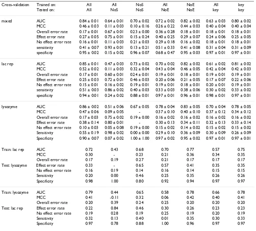
Overall, results suggest that structural information is more important than evolutionary information in predicting the functional consequences of a missense mutation in

Table 3: Results with a learned Bayesian network.

Cross-validation Trained on: All All NoS All NoE All key

Tested on: All NoS NoS NoE NoE key key

mixed AUC 0.84 ± 0.01 0.64 ± 0.01 0.70 ± 0.02 0.72 ± 0.02 0.82 ± 0.02 0.63 ± 0.03 0.80 ± 0.02 MCC 0.46 ± 0.03 0.11 ± 0.03 0.10 ± 0.16 0.26 ± 0.22 0.44 ± 0.03 0.40 ± 0.04 0.40 ± 0.04 Overall error rate 0.17 ± 0.01 0.67 ± 0.01 0.23 ± 0.00 0.36 ± 0.28 0.18 ± 0.01 0.18 ± 0.01 0.18 ± 0.01 Effect error rate 0.27 ± 0.05 0.75 ± 0.01 0.15 ± 0.24 0.40 ± 0.25 0.29 ± 0.07 0.24 ± 0.06 0.25 ± 0.05 No effect error rate 0.16 ± 0.01 0.11 ± 0.03 0.21 ± 0.03 0.29 ± 0.18 0.16 ± 0.02 0.18 ± 0.01 0.18 ± 0.01 sensitivity 0.41 ± 0.07 0.93 ± 0.01 0.13 ± 0.21 0.51 ± 0.33 0.41 ± 0.08 0.31 ± 0.04 0.31 ± 0.09 specificity 0.95 ± 0.02 0.15 ± 0.02 0.96 ± 0.07 0.68 ± 0.47 0.95 ± 0.03 0.97 ± 0.01 0.97 ± 0.01

lac rep AUC 0.85 ± 0.01 0.47 ± 0.03 0.73 ± 0.02 0.70 ± 0.02 0.82 ± 0.02 0.61 ± 0.02 0.81 ± 0.02 MCC 0.52 ± 0.02 0.11 ± 0.03 0.32 ± 0.04 0.43 ± 0.04 0.46 ± 0.05 0.42 ± 0.04 0.42 ± 0.03 Overall error rate 0.17 ± 0.01 0.60 ± 0.01 0.24 ± 0.01 0.19 ± 0.01 0.18 ± 0.01 0.19 ± 0.01 0.19 ± 0.01 Effect error rate 0.25 ± 0.03 0.72 ± 0.01 0.46 ± 0.03 0.20 ± 0.06 0.21 ± 0.05 0.17 ± 0.07 0.22 ± 0.06 No effect error rate 0.15 ± 0.01 0.16 ± 0.02 0.19 ± 0.01 0.19 ± 0.01 0.18 ± 0.01 0.20 ± 0.01 0.19 ± 0.01 sensitivity 0.51 ± 0.03 0.86 ± 0.02 0.40 ± 0.03 0.33 ± 0.03 0.38 ± 0.06 0.30 ± 0.02 0.33 ± 0.02 specificity 0.94 ± 0.01 0.24 ± 0.02 0.88 ± 0.01 0.97 ± 0.01 0.96 ± 0.01 0.98 ± 0.01 0.97 ± 0.01

lysozyme AUC 0.86 ± 0.02 0.51 ± 0.06 0.67 ± 0.05 0.78 ± 0.04 0.83 ± 0.05 0.70 ± 0.04 0.78 ± 0.05 MCC 0.47 ± 0.06 0.09 ± 0.05 - 0.37 ± 0.10 0.40 ± 0.10 0.37 ± 0.12 0.34 ± 0.12 Overall error rate 0.17 ± 0.03 0.75 ± 0.02 0.19 ± 0.00 0.16 ± 0.02 0.16 ± 0.02 0.16 ± 0.02 0.16 ± 0.02 Effect error rate 0.38 ± 0.14 0.80 ± 0.01 - 0.30 ± 0.13 0.34 ± 0.11 0.32 ± 0.13 0.33 ± 0.14 No effect error rate 0.10 ± 0.03 0.05 ± 0.08 0.19 ± 0.00 0.15 ± 0.02 0.14 ± 0.02 0.15 ± 0.02 0.15 ± 0.02 Sensitivity 0.55 ± 0.19 0.98 ± 0.02 0.00 ± 0.00 0.29 ± 0.10 0.36 ± 0.09 0.30 ± 0.09 0.26 ± 0.09 Specificity 0.90 ± 0.07 0.07 ± 0.02 1.00 ± 1.00 0.97 ± 0.02 0.95 ± 0.02 0.97 ± 0.01 0.97 ± 0.01

Train: lac rep AUC 0.72 0.43 0.68 0.70 0.77 0.57 0.75

MCC 0.30 - 0.23 0.21 0.36 0.34 0.35

Overall error rate 0.17 0.19 0.27 0.21 0.17 0.17 0.17 Test: lysozyme Effect error rate 0.33 - 0.65 0.57 0.41 0.35 0.35 No effect error rate 0.16 0.19 0.14 0.16 0.14 0.15 0.15

Sensitivity 0.20 0.00 0.46 0.25 0.35 0.26 0.26

Specificity 0.98 1.00 0.80 0.92 0.94 0.97 0.97

Train: lysozyme AUC 0.79 0.44 0.65 0.58 0.78 0.66 0.78

MCC 0.41 -0.11 0.32 0.06 0.42 0.40 0.41

Overall error rate 0.20 0.39 0.24 0.25 0.20 0.20 0.20 Test: lac rep Effect error rate 0.22 0.84 0.46 0.30 0.26 0.23 0.23 No effect error rate 0.19 0.28 0.19 0.25 0.19 0.20 0.19

Sensitivity 0.32 0.13 0.40 0.01 0.35 0.30 0.33

Specificity 0.97 0.78 0.88 1.00 0.96 0.97 0.97

both lac repressor and T4 lysozyme, for the dataset used. Indeed, although evolutionary information has some pre-dictive power, utilising only structural information appears to be sufficient for accurate prediction, compara-ble to that of the all:all model.

A note on structural flexibility

It has previously been suggested that the B-factor and neighbourhood B-factor of the native amino acid are the most important predictors of functional effects of SNPs [17]. However, the need to use B-factor information limits a method to structures from X-ray crystallography; such information is not available for NMR structures (although these do have their own internal flexibility measures). We found that removing the bf and nbf nodes from the all node network made little significant difference to overall performance with AUCs ranging from 0.80 to 0.83 in homogeneous cross-validation and 0.78 and 0.82 in het-erogeneous cross-validation (results not in Table). This suggests that accurate prediction is possible without using structural flexibility information, although that is not to say that structural flexibility is not important, rather, other variables have compensated effectively for its loss.

Learned structure

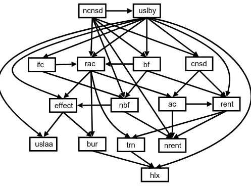
Using both the Bayesian and BIC scoring functions employed by the greedy search algorithm we learned structures from lac repressor and lysozyme datasets sepa-rately and the two datasets combined ('mixed'). As with the naïve Bayes classifier, we evaluated each structure using both homogeneous ten-fold and heterogeneous cross-validation. There was little significant difference in performance between the two scoring functions, or between structures learned on different datasets. The main difference was in the number of edges in the resulting DAGs. For our mixed dataset, there were 35 edges with BIC, and 48 with full Bayesian scoring. Using Occam's Razor, we prefer the simplest of equally good models, and take the Bayesian network structure learned from the mixed dataset, using the BIC scoring function, as our model structure , which is illustrated in Figure 2. With a harsher penalty for extra edges, the DAG learned using the BIC scoring function, should contain edges which are more likely to be biologically meaningful. It is important to note that the Bayesian networks with learned structure (or structure determined from conditional independence relations identified by an expert) capture the relationships between all the variables, and are not designed solely to discriminate for classification of a single variable based on the other variables. This is a significant advantage of the Bayesian network: we can infer the value of any varia-ble(s) based on the value of any other variable, so we have

constructed a model which can not only predict effect/no effect, but can infer the value of any of the attributes.

all:all

Little significant improvement in homogeneous cross val-idation performance was gained from using structure (Table 3, column 1) over the simple naïve structure (Table 2, column 1). This was because the naïve structure is spe-cifically designed for classification, whereas our learned structure is the 'best' structure for capturing the relation-ships between all of the variables. The learned structure performs as well in classification of effect as the naïve structure, but has the added advantage that it can be used to predict the values of any of the variables, from any of the other variables.

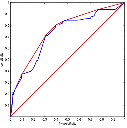
Structure appeared to perform worse than the naïve structure during heterogeneous cross-validation, espe-cially when trained on lac repressor and tested on lys-ozyme data. Here, AUC decreased from 0.80 to 0.72 despite lower effect error rates at the selected threshold (0.33 vs 0.52). The low AUC value of 0.72 may be decep-tive since a significant number of points on the ROC curve lie below the convex hull (Figure 3) and as such are non-optimal classifiers [32]. Therefore, measuring the per-formance of a classifier which represents a single point on both the ROC curve and the convex hull (circled in Figure 3) was more useful in this case. As described in Methods, we chose the point at cost ratio 3.0 (where false positives cost three times more than false negatives) as this helps balance the 'effect' and 'no effect' misclassification error rates (important in datasets such as ours that are biased towards negative examples). At this selected threshold, overall error (0.17) and effect error rate (0.33) were lower for structure than the naïve structure (0.20 and 0.52 respectively). However, MCC value was also lower (0.30 vs 0.40) and no effect error rate was higher (0.16 vs 0.10) which illustrates the difficulty in selecting a measure to compare different models not only between different studies but within the same study as well.

Missing structural information (all:noS and noS:noS)

The model learned from all the variables and tested using only evolutionary information (all:noS, Table 3, column 2) performed poorly achieving AUC values less than 0.50 (worse than random) and error rates above 0.75. Given the number of connections in and the potential for inferring the missing structural information in the test











data, the all:noS model was surprisingly worse than the noS:noS model (Table 3, column 3).

There could be a number of reasons for the poor perform-ance of the all:noS model. The model may have learned during training that structural information is more impor-tant to prediction than evolutionary information. Conse-quently, without structural information during testing, the model has problems since it has down-weighted the evolutionary nodes relative to the structural nodes. Alter-natively, it may not be possible to accurately infer values at the structural nodes from evolutionary information. By contrast, it is essential that the noS:noS model makes full use of the evolutionary information since structural infor-mation is unavailable in both training and testing. Even though cross validation results with noS:noS were worse than the all:all model with AUC values ranging from 0.65 – 0.73 and overall error rates up to 0.27, they were better

than the all:noS since full weight is given to the evolution-ary nodes.

Missing evolutionary information (all:noE and noE:noE)

When marginalising over unknown evolutionary varia-bles (all:noE, Table 3, column 4), predictions in most cases were comparable to the all:all model. However, poor results were achieved during homogeneous cross valida-tion on mixed data and heterogeneous cross validavalida-tion, especially training on lysozyme and testing on lac repres-sor data (AUC 0.58). In these cases, it appears that values at the evolutionary nodes with missing data could not be predicted accurately from the structural information dur-ing testdur-ing thus confusdur-ing the model. As expected, the noE:noE model trained and tested using structural varia-bles only performed as well as the all:all model across all cross validation tests (Table 3, column 5).

Learned Bayesian network structure

Figure 2

Learned Bayesian network structure . Learned Bayesian network structure (using greedy search with BIC scoring function from mixed dataset). Key to node labels is shown in Table 1.

uslby

effect

ac

rac

rent

nrent

bf

nbf

bur

_trn

hlx

cnsd

ncnsd

ifc

uslaa

Tolerance to incomplete training data

Bayesian networks are capable of learning model parame-ters from incomplete data. Here we test the tolerance of the Bayesian networks by training on incomplete data. In every training example, we hide n nodes (chosen ran-domly for each training case). We do this for the naïve Bayes classifier, and the learned structure , and vary n from 0 to 14. The CPTs are learned using the iterative EM algorithm on the missing values. Figure 4 shows the results of homogeneous cross-validation when trained on incomplete data from the 'mixed' dataset, and tested when all nodes are observed. Note that using this method, different sets of n nodes are chosen to have missing data between different training cases, therefore here we were testing the general ability of the Bayesian network to tol-erate incomplete data rather than the effect of when cer-tain nodes were missing data in all examples (as in the previous section).

Figure 4 shows that the performance of both the naïve and structures (measured by AUC value) were robust to incomplete training data, with an area under the ROC

curve of over 0.80 maintained even when nine of the fif-teen nodes were not observed in every example. With very sparse data (more than 9 nodes hidden), the naïve Bayes classifier performed better than the learned structure. This was probably because the conditional probability tables (CPTs) of the naïve structure only model the relationship of effect with each variable, whereas the CPTs of depend on the relationship between multiple variables. From Figure 2, we can see that a number of nodes are dependent on three variables in , which perhaps explains the performance decrease when the model is not trained on sets of four or more variables. For example, when 11 variables are missing, an AUC value of 0.73 is achieved by , whereas when 12 variables are missing, performance decreases to that of random classifier (AUC < 0.5). Nevertheless, overall tolerance to incomplete train-ing data by both Bayesian networks was encouragtrain-ing con-sidering the potential sparsity of either evolutionary and structural information for a significant number of pro-teins, especially structural genomics targets. Other machine learning methods such as SVMs or decision trees are unable to handle incomplete data in this way.

Training set size

In order to assess how much data is needed for training the Bayesian networks, sequential learning of the model parameters was performed. The 'mixed' dataset was divided into two. One half was used as the test validation









 Classifier performance

Figure 4

Classifier performance. Performance of naïve Bayes clas-sifier and structure with parameters learned from incom-plete data. The AUC (area under the ROC curve) is plotted against the number of nodes (n) randomly chosen to have missing data within the test examples.

0 1 2 3 4 5 6 7 8 9 10 11 12 13 14 0.4

0.5 0.6 0.7 0.8 0.9 1

Number of missing data in each training case

Area under ROC curve Naive Bayes classifier learned BN structure S



ROC curve for learned structure

Figure 3

ROC curve for learned structure . ROC curve for learned structure trained on lac repressor, tested on lys-ozyme. The blue line is the ROC curve. The red line is the convex hull of the ROC curve. The circled point which lies on both of these curves is the classifier with the selected threshold (cost ratio = 3.0).

0 0.1 0.2 0.3 0.4 0.5 0.6 0.7 0.8 0.9 1 0

0.1 0.2 0.3 0.4 0.5 0.6 0.7 0.8 0.9 1

1−specificity

sensitivity

set, and the Bayesian networks were trained on the other half. Figure 5 shows a plot of training set size vs. classifier performance, measured using area under the ROC curve. The result is as expected. The naïve model (with its 43 parameters) gradually improves its performance as its parameters are sequentially learned, with excellent per-formance after 400 examples (and good after as few as 50). The learned BN structure has 182 free parameters and it out performs the naïve classifier after 1000 training examples.

Interpreting the structures

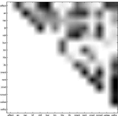
The learned structure is one of many Markov equiva-lent structures which could have been learned from this data. There are also many other network structures which could suitably encode the relationships between the vari-ables. Using Markov chain Monte Carlo (MCMC) meth-ods, we constructed a set of 'good' model structures, and averaged over these models to form a posterior distribu-tion of model structures. Figure 6 shows a plot of the fre-quency of connections made in the set of 'good' structures from ten runs of the MCMC simulation over 10000 sam-ples, after a 'burnin' of 1000 samples. The darker squares indicate a higher observed frequency of an edge connect-ing each pair of nodes. From this, one can identify strong

relationships between highly correlated variables. The use of MCMC methods to study the posterior distri-bution over networks has the advantage of revealing rela-tionships between the input variables. For instance, in Figure 6, the top row shows which variables are most strongly related to effect, and this is used later to develop simplified classifiers.

However, biologically meaningful relationships between the other variables are also revealed. With the exception of the trivial relationship between ac and rac, the second row of Figure 6 shows strong links between ac, nrent, and rent, reflecting a well known biochemical relationship between solvent accessibility of residues and phylogenetic variabil-ity: the solvent exposed surface loops of protein structures show greater evolutionary variability than the unexposed hydrophobic core residues. Similar effects that concur with known protein chemistry relate measures of flexibil-ity (nbf, bf) to phylogenetic variability. Equally under-standable are the strong link between G and P residues in turns (trn) and evolutionary conservation at the specific sequence position of G/P (indicated by rent, cnsd) but not to a neighbourhood measure (nrent, ncnsd), and the rela-tionship between protein interface positions (ifc) and neighbourhood flexibility measures (nbf).

From Figure 6, one can see that the effect node has the strongest relationships with bur, nbf, ac, uslaa, and uslby (in





Posterior distribution of relationships

Figure 6

Posterior distribution of relationships. Strength of rela-tionships between variables, identified through analysis of edges connecting pairs of nodes in MCMC structure learning. A dark square indicates a strong relationship; a white square a weak relationship.

effect ac rac bf nbf bur trn hlx ifc nrent rent cnsd ncnsd uslaa uslby effect

ac rac bf nbf bur trn hlx ifc nrent rent cnsd ncnsd uslaa uslby

Training set size

Figure 5

Training set size. Performance of naïve Bayes classifier and structure with parameters learned sequentially. The AUC (area under the ROC curve) is plotted against the number of training examples.

0 500 1000 1500 2000

0.65 0.7 0.75 0.8

Training set size

Area under ROC curve

Naive Bayes classifier learned BN structure S

descending order). There are very few direct connections between effect and trn, hlx, ifc, cnsd, and ncnsd. As expected, nodes such as bf and nbf, and rent and nrent are highly cor-related, which suggests some redundancy within the net-work and one node could be used to predict the value of the other. Both structural and evolutionary information are represented by the nodes most frequently directly con-nected to effect, although the top three most common nodes, bur, nbf and ac, represent only structural informa-tion. This, together with the strong performance of the Bayes classifier without evolutionary information (Table 2, columns 4 and 5), suggests that evolutionary properties of the mutated residue have little direct influence on pre-diction if structural information is present.

Our finding that solvent accessible area of the native amino acid, whether the amino acid is charged at a buried site, and the flexibility of its structural neighbourhood are all important predictors of effect agrees to some extent with Chasman and Adams (2001) who found that struc-ture based accessibility and B-factor feastruc-tures have the most discriminatory power. The strong performance of accessibility measures probably reflects the finding of [5] and [6] that mutations affecting the hydrophobic core are more likely to destabilise the protein and thus affect func-tion. Perhaps mutations on the surface are more likely affect function if they are conserved, as suggested by the strong relationship between accessibility and phyloge-netic entropy (ac with rent and nrent). Conversely, whether or not the mutation breaks either a helix or turn does not appear to be critical to predicting effect although, again, secondary structure information may become more powerful when used in conjunction with other features.

A simplified Bayesian network

Whilst the nodes directly connected to the effect node are not essential to prediction if certain other nodes are present (as demonstrated by the removal of the structural flexibility nodes nbf and bf, with no significant loss of per-formance), in theory, the value of the effect node can be predicted using only the nodes which are directly con-nected to it in the learned structures. The other variables become d-separated from effect; i.e. with a structure, and the conditional independence relations it implies, the effect node is conditionally dependent on only the nodes it is connected to when they are observed.

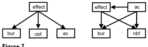
We tested this hypothesis by constructing two simple four node networks: a naïve structure (Figure 7a), and structure

3 (Figure 7b) learned using the greedy search algorithm

and the BIC scoring function as above. These networks consisted of only the three nodes, bur, nbf and ac, with the strongest relationships with effect as shown in Figure 6.

Across all cross-validation tests, the four node naïve Bayes classifier trained and tested using only the three key varia-bles (key:key, Table 2, final column) performed extremely well with only a minor decrease in performance over the all:all model. In homogeneous cross validation, AUC val-ues ranged from 0.77 to 0.80 and the maximum overall error rate was just 0.21. In heterogeneous cross validation tests, the AUC also remained high (0.77 and 0.79) with overall error rates as low as 0.16 for training on lac repres-sor and testing on lysozyme data. There were no signifi-cant differences between the performance of the four node learned structure (key:key, Table 3, final column) and that of the naïve structure, which suggests little value in the connections between variables.

Conclusion

We have applied Bayesian networks to the task of predict-ing whether or not missense mutations will affect protein function with comparable performance to other machine learning methods. However, the strength of the Bayesian network lies in its ability to handle incomplete data and to encode relationships between variables; both of which were exploited here to derive some biological insight into how a missense mutation affects protein function.

A number of models were learned in this work. Due to the unbalanced datasets we analysed ROC curves and selected a suitable cost ratio in order to choose a probability threshold for the classifiers. This allowed us to compare classifiers in a meaningful way. From this analysis we con-cluded that a naïve network structure is sufficient for accu-rate prediction of the effect of a missense mutation with AUC values around 0.80. We also found that the structural environment of the amino acid is a far better predictor of the functional consequences of a missense mutation than phylogenetic information. This was demonstrated by the more accurate performance of a naïve classifier that just uses structural information compared to that which uses just evolutionary information. There were no significant performance gains when using a learned network struc-ture, however the learned structure did allow

relation-

Simplified Bayesian networks

Figure 7

Simplified Bayesian networks. Four node networks using the three key variables shown to have the strongest relation-ship with the effect. (a) Naïve Bayes classifier, (b) learned Bayesian network structure ₃.

effect

ac nbf

bur

effect ac

nbf bur

ships between variables to be analysed, in particular by analysing the posterior distribution of model structures, we found the top three strongest connections with the effect node all involved structural nodes. With this in mind, we derived a simplified Bayesian network that used just these three structural descriptors (solvent accessible area of the native amino acid, whether the amino acid is charged at a buried site, and the flexibility of its structural neighbourhood) without significant decrease in perform-ance. Given the importance of structure, it would be inter-esting to learn if certain amino acid changes are more predictive of effect than others. For example, both cysteine, which forms disulphide bridges, and proline, with its unique ring structure, are often critical to the integrity of a protein structure so one would expect a mutation involving either of these residues to change the structure significantly. This will provide the basis for future work.

Methods

Evaluation measures

A number of measures were applied to evaluate each clas-sifier: error rates (fraction of mis-classified examples), sen-sitivity (true positive rate) and specificity (true negative rate). We also used Matthews' correlation coefficient (MCC), which is a correlation measure designed for com-parison of unbalanced datasets such as ours. A value of +1 indicates perfect classification, and -1 indicates misclassi-fication of every example. The MCC is defined as:

where TP are true positives, TN are true negatives, FP are false positives, and FN are false negatives obtained from evaluating the classifier on the test data.

Since we have a Bayesian network classifier, with a proba-bility associated with each classification, the metrics above depend on the value of the classification threshold p that is used. To assess performance across a range of val-ues of the probability threshold we plotted a receiver operator characteristic (ROC) curve. The ROC curve is a plot of the sensitivity versus (1-specificity) for all feasible ratios of costs associated with misclassification errors (equivalent to plotting true positive rate versus false posi-tive rate). The area under the curve (AUC) is a measure of the performance of a binary classifier. A classifier no better than random gives an AUC of 0.5, a perfect classifier gives an AUC of 1.0.

Choosing a classification threshold

In order to perform a fair comparison of classifiers, we choose the classification threshold p, represented by a point on the ROC curve for which the curve has a gradient

(ΔTPrate/ΔFPrate) of CFP/CFN – the ratio of costs between

False Positives and False Negatives, and which is closest to the point (0, 1). In this work we use a cost ratio of 3.0, due to the unbalanced nature of the datasets containing 3742 mutations which have no effect on protein function and 1135 which do effect protein function. This is close to 3:1, and by weighting the cost of a false positive, C_FP, as three times more costly (to the classifier) than a false negative, CFN, we obtain a classifier with reasonably well balanced

error rates. This means the classifier is less likely to predict everything as an effect (than with an equal cost ratio of 1.0) and make many false positive errors, which would give a high effect error rate. (Without doing this, we may be comparing classifiers with very different properties. i.e. ones with quite different specificities and sensitivities). The method is applied to the ROC curves obtained from the probabilistic classification scheme and we present the results for the classification threshold p corresponding to the point on the convex hull of the ROC curve where the gradient is closest 3.0. (We choose a point on the convex hull since any point on the ROC curve not on the convex hull is a non-optimal classifier [32]).

Data discretization

There were a number of challenges buried in these data. Continuous data was non-Gaussian, making it unsuitable for modelling as a continuous Gaussian node in a Baye-sian network. There were also no obvious boundaries at which to separate the data into discrete categories. Our solution was to fit a number of Gaussians to the data using an Expectation-Maximisation based algorithm that automatically chooses the number of classes. It begins with one Gaussian, and iteratively splits the Gaussian with the largest weight, until adding extra classes does not increase the maximum likelihood of the model. Full details are provided below. This allowed us to form dis-crete classes from continuous data, which gave better per-formance than simply splitting the data into three classes of equal range (results not shown). We therefore used this strategy in all our analyses.

The E-M algorithm

The Expectation Maximisation algorithm is a well estab-lished efficient algorithm for fitting Gaussian mixture models to data. The main draw-back of the algorithm is its sensitivity to initialisation, and the need for multiple runs with different numbers of mixtures in order to choose the maximum likelihood model. Here we present a adapta-tion to the method which is deterministic and automati-cally chooses the number of Gaussians. It begins with one Gaussian, and iteratively splits the Gaussian with the larg-est weight, until adding extra mixtures does not increase the maximum likelihood of the model. Given a data set X

= {x1,..., xN} of N cases of d-dimensional data, a single

cluster μ1 is initialised at the mean of the data. A Gaussian

MCC TP TN FP FN

TP FP TP FN TN FP TN FN

= × − ×

+ + + +

( ) ( )

with diagonal covariance equal to the standard deviation of the data in each dimension is placed at μ1 The weight of

this cluster is set to one p(j = 1) = 1.

The probability p(j|xi) is calculated for each data point xi.

For a set of j mixtures, the update equations follow. These are iteratively performed until the maximum likelihood is reached, i.e. ML = log∑i∑jp(j|xi)

E-step:

M-step:

When the ML stops increasing, the Gaussian with the larg-est weight p(j) described by μj and sj is split into two

Gaus-sians at and , each with the same covariance sj. The

new Gaussians are placed +/- a distance of the largest eigenvalue in the direction of the principle eigenvector of the covariance matrix sj from μj. (The Gaussians are then

renamed). The EM steps above are performed until the maximum likelihood configuration is reached. This proc-ess is repeated until the ML score is no higher than with one less Gaussian. At each stage, the centres and covari-ances of the Gaussians are saved. Thus the algorithm ter-minates with a set of Gaussians that are at best no better than the set at the previous stage with one less Gaussian, so the saved set from the previous stage is used.

Classification of each data point xi is taken as a hard

clas-sification into the most likely class given by argj max

p(j|xi).

Authors' contributions

CJN carried out the study, CAM assisted with data sets and result interpretation, JRB advised on biological aspects and result interpretation, AJB and DRW, suggested the study and assisted with result interpretation. All authors approved the final manuscript.

Acknowledgements

We would like to thank the BBSRC who funded this research under grant BBSB16585.

References

1. Thorisson GA, Stein LD: The SNP Consortium website: past, present and future. Nucl Acids Res 2003, 31:124-127.

2. The SNP Consortium website [http://snp.cshl.org]

3. Sherry ST, Ward MH, Kholodov M, Baker J, Phan L, Smigielski EM, Sirotkin K: dbSNP: the NCBI database of genetic variation.

Nucleic Acids Res 2001, 29:308-311.

4. NCBI dbSNP [http://www.ncbi.nlm.nih.gov/SNP]

5. Wang Z, Moult J: SNPs, protein structure, and disease. Hum Mutat 2001, 17:263-270.

6. Ramensky V, Bork P, Sunyaev S: Human nonsynonymous SNPs: server and survey. Nucleic Acids Res 2002, 30:3894-3900. 7. Chasman D, Adams RM: Predicting the Functional

Conse-quences of Non-synonymous Single Nucleotide Polymor-phisms: Structure-based Assessment of Amino Acid Variation. J Mol Biol 2001, 307:683-706.

8. Ferrer-Costa C, Orozco M, de la Cruz X: Characterization of dis-ease-associated single amino acid polymorphisms in terms of sequence and structure properties. J Mol Biol 2002, 315:771-786.

9. Ng PC, Henikoff S: Predicting deleterious amino acid substitu-tions. Genome Res 2001, 11:863-874.

10. Krishnan VG, Westhead DR: A comparative study of machine learning methods to predict the effects of single nucleotide polymorphisms on protein function. Bioinformatics 2003, 19(17):2199-2209.

11. Herrgard S, Cammer SA, Hoffman BT, Knutson S, Gallina M, Speir JA, Fetrow JS, Baxter SM: Prediction of deleterious functional effects of amino acid mutations using a library of structure-based function descriptors. Proteins: Structure, Function, and Genet-ics 2003, 53(4):806-816.

12. Sunyaev S, Ramensky V, Koch I, Lathe W III, Kondrashov AS, Bork P: Prediction of deleterious human alleles. Hum Mol Genet 2001, 10:591-597.

13. Ng PC, Henikoff S: SIFT: predicting amino acid changes that affect protein function. Nucl Acids Res 2003, 31(13):3812-3814. 14. Saunders CT, Baker D: Evaluation of structural and

evolution-ary contributions to deleterious mutation prediction. J Mol Biol 2002, 322:891-901.

15. Bao L, Cui Y: Prediction of the phenotypic effects of non-syn-onymous single nucleotide polymorphisms using structural and evolutionary information. Bioinformatics 2005, 21(10):2185-2190.

16. Cai Z, Tsung EF, Marinescu VD, Ramoni MF, Riva A, Kohane IS: Baye-sian Approach to Discovering Pathogenic SNPs in Con-served Protein Domains. Human Mutation 2004, 24:178-184. 17. Verzilli CJ, Whittaker JC, Stallard N, Chasman D: A hierarchical

Bayesian model for predicting the functional consequences of amino-acid polymorphisms. Applied Statistics 2005, 54:191-206.

18. Beaumont MA, Rannala B: The Bayesian Revolution in Genetics.

Nature Reviews Genetics 2004, 5:251-261.

19. Friedman N: Inferring Cellular Networks Using Probabilistic Graphical Models. Science 2004, 303:799-805.

20. Husmeier D, Dybowski R, Eds: SR: Probabilistic Modeling in Bioinformat-ics and Medical InformatBioinformat-ics Springer; 2005.

21. Jordan MI: Learning in Graphical Models Kluwer Academic; 1998. 22. Jensen FV: Bayesian Networks and Decision Graphs Springer; 2001. 23. Pearl J: Causality: models, reasoning and inference Cambridge; 2000. 24. Needham CJ, Bradford JR, Bulpitt AJ, Westhead DR: Inference in

Bayesian networks. Nature Biotechnology 2006, 24:51-53.

µµ

µµ µµ

1 ₁

1 ₁ 1 1

1 1 1 1 = = − − = = = =

∑

∑

i i T

i N

x

s (x )(x )

( )

p j p j p j p x p j i i i i _d j

i j j

( | ) ( ) ( | ) ( )

( | )

( )

exp ( )

x x

x

s

x s

=

= 1 − −

2 1 2 2 1 2 π µµ −− = − ⎛ ⎝ ⎜ ⎞_⎠⎟ =

∑

i j T

i i

N

p j p j

µµ

µµ

µµ

j _iN i i

j _iN i i j i j T

p j p j

p j p j

= = − − = =

∑

∑

s x x x µ

Publish with BioMed Central _{and every} scientist can read your work free of charge

"BioMed Central will be the most significant development for disseminating the results of biomedical researc h in our lifetime."

Sir Paul Nurse, Cancer Research UK

Your research papers will be:

available free of charge to the entire biomedical community peer reviewed and published immediately upon acceptance cited in PubMed and archived on PubMed Central yours — you keep the copyright

Submit your manuscript here:

http://www.biomedcentral.com/info/publishing_adv.asp

BioMed_central

25. Murphy KP: The Bayes Net Toolbox for Matlab. Computing Sci-ence and Statistics 2001:331-350.

26. Leray P, Francois O: BNT Structure Learning Package: Docu-mentation and Experiments. Tech. rep., Laboratoire PSI, Univer-sité et INSA de Rouen; 2004.

27. Heckerman D: A tutorial on learning with Bayesian networks. In Learning in Graphical Models Edited by: Jordan MI. Kluwer Academic; 1998:301-354.

28. Markiewicz P, Kleina LG, Cruz C, Ehret S, Miller JH: Genetic studies of the lac repressor. XIV. Analysis of 4000 altered Esherichia coli lac repressors reveals essential and non-essential resi-dues, as well as 'spacers' which do not require a specific sequence. J Mol Biol 1994, 240:421-433.

29. Suckow J, Markiewicz P, Kleina LG, Miller J, Kisters-Woike B, Muller-Hill B: Genetic studies of the lac repressor. XV: 4000 single amino acid substitutions and analysis of the resulting pheno-types on the basis of the protein structure. J Mol Biol 1996, 261:509-523.

30. Alber T, Sun DP, Nye JA, Muchmore DC, Matthews BW: Temper-ature sensitive mutations of bacteriophage T4 lysozyme occur at sites with low mobility and low slovent accessibility in the folded protein. Biochemistry 1987, 26:3754-3758. 31. Rennell D, Bouvier SE, Hardy LW, Poteete AR: Systematic

muta-tion of bacteriophage T4 lysozyme. J Mol Biol 1991, 222:67-88. 32. Fawcett T: ROC Graphs: Notes and Practical Considerations