Article
Numerical Study of the Oregonator Models on the
Basis of the Two-Phase Rozenbrock’s Method with
Complex Coefficients
Rustam D. Ikramov
a,* and Svetlana A. Mustafina
bBashkir State University, Russian Federation
E-mail: a[email protected](Corresponding author), b[email protected]
Abstract. Chemical transformations typically occur according to multiphase schemes. Changes in the concentrations of the starting materials and intermediates with time are not always described with increasing or decreasing functions. A detailed study of a complex process kinetics showed that at the presence of feedback far from equilibrium there may occur vibrational modes - periodic increase or decrease in the concentration of one of the components in time. In a numerical study of oscillating reactions there appears a problem in solving a rigid system of typical differential equations. The purpose of this study is to develop an algorithm and a program to solve the direct kinetic problem and to investigate multicomponent chemical systems with complex nonlinear dynamics.
Keywords: Belousov-Zhabotinsky’s reaction, critical reaction, deactivation, Oregonator, oscillations.
ENGINEERING JOURNAL Volume 20 Issue 1 Received 8 February 2015
1.
Introduction
Among the numerous oscillating chemical and biochemical reactions the most famous class of reactions is the class first discovered by the Russian scientists B.P. Belousov and A.M. Zhabotinsky [1]. Belousov-Zhabotinsky’s reaction has been studied in hundreds of world laboratories in vessels of various shapes, in a flow, in porous environments, etc.
The mechanism of Belousov-Zhabotinsky’s reaction has more than 80 phases. Due to this fact the investigation of the reactions patterns, solutions of the direct and inverse problems as well as the optimization problems are often impossible. In paper [2] there is proposed a simple and abstract model of Belousov-Zhabotinsky’s reaction, which turned out to preserve the most important features of this reaction. Such a simplified scheme has been called Oregonator [2].
Model Oregonator describing the behavior of Belousov-Zhabotinsky reaction, found its use not only in chemistry but also in other sciences, such as medicine, geology, and others. For example, the wave structures of the oscillations of the heart musclehave a similar kind of oscillations. Therefore, the study of the model Oregonator and a study of the Belousov-Zhabotinsky reaction is relevant at the moment.
2.
Data Analyses
We consider several variants of models of Belousov-Zhabotinsky’s oscillatory reaction. We assume that the reaction is carried out in a closed vessel. Then the reaction scheme can be presented as follows [3]:
, ,
2 ,
2 ,
,
A Y X
X Y P
B X X Z
X Q Z fY (1)
where A and B – raw reactants, P and Q – products, X , Y , Z – intermediates: HBrO2 , Br and
( )
Ce IV correspondingly. Differential equations describing the dynamics of Belousov-Zhabotinsky’s
reaction (according to a simplified Oregonator scheme) has the following form [4]:
2
1 2 3 4
1 2 5
3 5
[ ]
[ ][ ] [ ][ ] [ ][ ] 2 [ ] ,
[ ]
[ ][ ] [ ][ ] [ ],
[ ]
[ ][ ] [ ],
d X
k A Y k X Y k B X k X
dt d Y
k A Y k X Y fk Z
dt d Z
k B X k Z
dt
(2)
where k1 1.34mole/s,
9 2 1.6 10
k mole/s, k3 8 103 mole/s, k4 4 107 mole/s, A0.06 mole, 0.06
B mole. Stoichiometric factor f and rate constant k5 are parameters related to the consumption
of reactants which can be varied [5].
System (2) is characterized by high rigidness coefficient, calculated according to the formula [6]
max(Re( )) ( ) , min(Re( )) i i t (3)
where i – eigenvalues of the Jacobi matrix of the system of differential equations along its solutions and Re( )i 0 . The rigidness coefficient ( )t for system (2) exceeds
6
1.4 10 [7].
Thus, for direct kinetic problem Eq. (2) explicit schemes for solving typical differential equations become inapplicable [8]. Therefore, the only possible way to solve problem Eq. (2) is to use implicit methods.
2 , , 2 , , 2 , 0.462 .
A X W
A Y X P
X Y P
C W X Z
X A P
Z C Y
(4)
This reaction involves 7 substances: A BrO3
, CM n( ) – ion of a metal catalyst, PHOBr,
2
W BrO , XHBrO2 , Y Br
, ZM n( 1) – an oxidized form of the ion of a metal catalyst. Let’s mark the concentration of the reagents in the following way: c1 [BrO3]
, c2 [Br ]
, c3 [M n( )] ,
4 [ 2]
c HBrO , c5[HOBr], c6 [BrO2], c7 [M n( 1)] . Since reaction (4) takes place in a constant
volume isothermal reactor with metabolism, then the corresponding system of differential equations consists of equations of the form:
1 1 3 5 1 1
2 1 2 6 2 2
3 4 6 3 3
4 1 2 3 4 5 4 4
5 1 2 5 5 5
6 3 4 6 6
7 4 6 7 7
( ) / ,
0.462 ( ) / ,
( ) / ,
2 ( ) / ,
2 ( ) / ,
2 ( ) / ,
( ) / , p p p p p p p
c v v v c c
c v v v c c
c v v c c
c v v v v v c c
c v v v c c
c v v c c
c v v c c
(5)
where / is the time of the mixture in the reactor, – reactor volume, – volumetric flow rate of the mixture through the reactor, vi, (i1..6) are given by:
1 1 1 2 1 4 5 2 2 2 2 4 2 5 2 3 3 1 4 3 6 4 4 3 6 4 4 7
2
5 5 4 5 1 5 6 6 7
, , , , , .
v k c c k c c
v k c c k c
v k c c k c
v k c c k c c
v k c k c c
v k c
Kinetic constants take the following values: k10.084 mole/s,
3 3 2 10
k mole/s, k3 2 103
mole/s, mole/s, 5
4 1.3 10
k mole/s, k5 4 104 mole/s, k6 0.65 mole/s,
4 1 10
k mole/s,
5 2 5 10
k mole/s, k3 2 107 mole/s, k4 2.4 10 7 mole/s. Initial conditions are given in the form
0
(0)
с с .
After checking the rigidness of the system of differential equations (5), we obtain that 5
( )t 4.5 10
[10].
Thus, for a numerical solution of Eq. (2) and Eq. (5) it is necessary to develop an algorithm for solving rigid problems with a wide range of sustainability.
Rosenbrock schemes - a family of methods for solving stiff problems, based on the diagonal implicit methods of Runge-Kutta. Some schemes of this family have increased reliability. In terms of stability, they do not concede implicit methods, but transition to the next time layer is obtained by the solution of system of linear equations with a finite number of steps. Initially, methods were proposed in 1963 by Rosenbrok to circumvent the problem of rigidness.
of Rosenbrock’s method for a transition to a new time layer require some solutions of a linear system of equations with a well-conditioned matrix which avoids iterations.
The use of complex coefficients is a non-trivial process to obtain the schemes with better accuracy and stability compared to the scheme with real coefficients. The number of parameters of the schemes is actually doubled.
Rosenbrock’s methods can take form [13] in the simplest case:
1 Re( 1 1 2 2)
n n
y y b g b g , (6)
where g1 and g2 are obtained from the relevant systems of linear equations:
1 1
2 1 2 1
[ ( )] ( ),
[ ( Re( ))] ( Re( )).
y n n
y n n
E h f y g hf y
E h f y h ag g hf y h dg
(7)
Here yn – direct numerical solution of the kinetic problem in a time moment t , h – time step, E – identity matrix, fy – Jacobi matrix of system (2) and system (5), 1 , 2, b1, b2, a and d – complex
parameters defining the properties of the scheme. In [13], the following values of the parameters of the method are given:
1 2 1 2 0.09705 0.14418i, 0.18866 0.06177i, 0.04833-0.32059i, 0.95166-1.69677i, 0.53597-0.96659i, 0.17308-0.16940i. b b a d
With appropriate parameters Rosenbrock’s scheme is L1-stable [14, 15].
The complexity of the algorithm is in the work with complex numbers and matrices of complex numbers. To find vectors g1 and g2 we have to solve a system of linear algebraic equations with complex
numbers. We have to move from complex numbers to real numbers when realizing the algorithm on a computer. To do this, we introduce the notation for finding vector g1 (vector g2 is similar):
1
[ y( n)]
А E h f y – complex matrix, Bhf y( n) – real vector.
First equation of system (7) can be represented in a matrix form:
1 .
Аg B (8)
Since matrix A and vector g1 contain complex numbers, then Eq. (8) can be represented as follows:
1 1
(Аre iAim)(gre igim)(Bre i0),
where Аre , g1re – real part of complex matrix A and vector g1 , Aim , g1im – corresponding complex parts of matrix A and vector g1, i – an imaginary unit.
To find vector g1 it is necessary to solve a system of equations
1 1
1 1
,
0.
re re im im re
im re re im
A g A g B
A g A g
(9)
Its solution can be written in the following way:
1 1 1 1 1 1 ( ), ( ) .
re im re im
im re im re im re
g A A g
g A A A A B
And we can obtain an explicit formula for the transition to the next time layer by substituting the parameters g1 and
2
g in the general equation of the method (6).
3.
Discussion
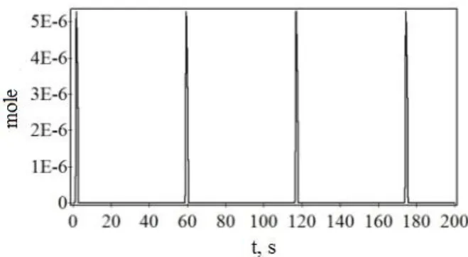
The results of the integration of the system (2) with initial conditions 11 0
[ ]X 5 10 mole, [ ]Y 0 3 107
mole, 8
0
3
10
h . The system of differential equations (2) is characterized by periodic changes of concentrations
with period T57.58c.
Fig. 1. Oscillating values of X reactant concentrations in reaction (2).
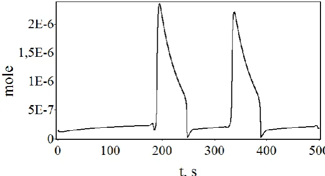
Fig. 2. Oscillating values of Y reactant concentrations in reaction (2).
[image:5.595.131.461.118.299.2] [image:5.595.133.458.330.502.2] [image:5.595.128.463.538.717.2]The results of the integration of the system (5) with initial conditions с10.1387 mole, 7
2 1.534 10
с mole, 4
3 1.176 10
с mole, 8
4 3.165 10
с mole, 4
5 1.956 10
с mole,
7
6 5.814 10
с mole, 6
7 6.31 10
с mole are given in Figs. 4–10 [17, 18]. The integration step is 3
10 .
h
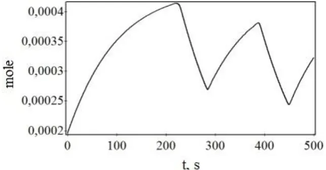
According to Figs. 4–10 we can see that kinetic curve of reagent c2, c3
,
c4, c6,
c7 is characterized by acomplex periodic oscillation mode and kinetic curve of reagent с5 by a quasisinusoidal oscillation [19, 20].
Fig. 4. Fluctuating values of c1 reagent concentration in reaction (5).
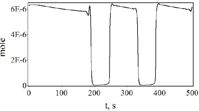
[image:6.595.134.452.191.364.2] [image:6.595.129.453.402.577.2]Fig. 6 Fluctuating values of c3 reagent concentration in reaction (5).
Fig. 7. Fluctuating values of c4 reagent concentration in reaction (5).
[image:7.595.130.461.290.464.2] [image:7.595.136.458.496.664.2]Fig. 9. Fluctuating values of c6 reagent concentration in reaction (5).
Fig. 10. Fluctuating values of c7 reagent concentration in reaction (5).
4.
C
onclusion
The article gives an algorithm for solving the direct kinetic problem based on Rosenbrock’s implicit schemes with complex coefficients. An algorithm test has been performed on the famous Belousov-Zhabotinsky’s reaction provided with the models taking into account the reactions in a closed and in an isothermal reactor of a constant volume.
A numerical simulation of Belousov-Zhabotinsky’s reaction has showed that periodic oscillations of reactant concentrations with period of T57, 58c can exist in a closed system. Simultaneously, fluctuations in concentrations can be represented by quasi-sinusoidal and complex periodic modes in an isothermal reactor.
There has been worked out a program providing a numerical study of oscillatory reactions in Object Pascal in Lazarus.
References
[1] B. Belousov, “Periodically acting reaction and its mechanism,” in Sbornik referatov po adiotsionnoi meditsine. Moscow: Medgiz, 1951, pp. 145–147.
[2] R. J. Field and R. M. Noyes, “Oscillations in chemical systems. IV. Limit cycle behavior in a model of a real chemical reaction,” Journal of Chemical Physics, vol. 60, no. 5, pp. 1877–1884, 1974.
[image:8.595.135.457.79.255.2] [image:8.595.137.464.290.473.2][4] M. V. Vol'kenshtejn, “Reakcia Belousova-Zhabotinskogo” in Biofizika. Moscow: Nauka, 1988, ch. 16, sec.2, pp. 515–521.
[5] A. M. Zhabotinsky, “Avtokolebatelnie khimicheskie reakcii v gomogennom rastvore. Kolebatelnie reakcii okisleniya bromatom,” in Koncentracionnye avtokolebanija. Moscow: Nauka, 1974, ch.4, pp. 87–113. [6] P. D. Shirkov, “Optimalno zatuhaushie skhemi s kompleksnimi koefficientami dlya zhestkih system
ODU,” Matematicheskoe modelirovanie, vol. 4, no. 8, pp. 47–57, 1992.
[7] J. D. Lambert, Numerical Methods for Ordinary Differential Systems. New York: Wiley, 1992, p. 304.
[8] G. A. Limonov, “Development of Rosenbrock’s two-phase schemes with complex coefficients and their application in the problems of periodic nanostructures modeling,” Ph.D. Thesis, Ural Federal Institute, Ekaterinburg, Russia, 2010.
[9] [9] R. Ikramov and S. Mustafina, “Chislennoe issledovanie modelej oregonatora s ispol''zovaniem dvuhstadijnogo metoda rozenbroka s kompleksnymi kojefficientami,” Informacionnye tehnologii modelirovanija i upravlenija, vol. 3, no. 87, pp. 211–217, 2014.
[10] R. D. Ikramov and S. A. Mustafina, “Numerical research of oscillatory processes in chemical kinetics by Rosenbrock’s method with complex coefficients,” Mejdunarodnii nauchno-issledovatelskii zhurnal, vol. 4, no. 23, pp. 12–14, 2014.
[11] A. B. Alshin, E. A. Alshina, and A. G. Limonov, “Dvuhstadiinie kompleksnie skhemi Rozenbroka dlya zhestkih system,” Zhurnal vichislitelnoi matematiki i matematicheskoi fiziki, vol. 49, no. 2, pp. 270–287, 2011.
[12] O. V. Noskov, “Chislennoe modelirovanie slozhnih kolebatelnih rezhimov v reakcii Belousova-Zhabotinskogo,” Ph.D. dissertation, Bashkir State University, Ufa, Russia, 1993.
[13] E. A. Novikov, “Numerical modelling of a modified Oregonator with method (2,1) of rigid problem solutions,” Computation methods and programming, vol. 11, pp. 281–288, 2010.
[14] R. D. Ikramov and S. A. Mustafina “Numerical modeling of ocsillating reactions based on Rosenbrock method with complex coefficients,” in Mejdisciplinarnie issledovaniya v oblasti matematicheskogo modelirovaniya i informatiki, Ul’yanovsk, Russia, 2014, pp. 78–83.
[15] R. D. Ikramov and S. A. Mustafina, “Semi-analytical approach to solving stiff systems of differential equations of the oscillating model of the Belousov-Zhabotinsky reaction,” in Matematicheskoe modelirovanie protsesov i system, Sterlitamak, Bashortostan Republic, Russia, 2014, pp.70–76.
[16] R. D. Ikramov and S. A. Mustafina, “Numerical modeling of oscillating reactions based on Rosenbrock’s method with real coefficients,” Zhurnal Srednevolzhskogo matematicheskogo soobshestva, vol. 16, no. 1, pp. 71–75, 2014.
[17] E. A. Novikov, L. V. Knaub, and A. E. Novikov, “Chislennoe modelirovanie Oregonatora trehstadiinimi metodami,” Modelirovanie system, vol. 3, no. 33, pp. 59–68, 2012.
[18] R. Ikramov and S. Mustafina, “Numerical study of the Belousov-Jabotinsky’s reaction models on the basis of the two-phase Rozenbrock’s method with complex coefficients,” International Journal of Applied Engineering Research, vol. 9, no. 22, pp 12797–12801, 2014.
[19] R. Ikramov and S. Mustafina, “Chislennoe issledovanie modelej reakcii belousova-zhabotinskogo na osnove dvuhstadijnogo metoda rozenbroka s kompleksnymi kojefficientami,” Sistemy upravlenija i informacionnye tehnologii, vol. 2, no. 56, pp. 11–14, 2014.