Brendan van Rooyen
A thesis submitted for the degree of
Doctor of Philosophy
A great many people and institutions have helped me complete this thesis. Firstly, I would like to thank my parents Karen and Bruce, without their input I can safely say I would not be in this position! I was very kindly supported by both the Australian National University and National ICT Australia. I thank both for creating a fantas-tic environment for learning. I would like to thank all of my friends from both the ANU and NICTA, including but not limited to Lachlan Chislett, Tom Chen, Kiara Bruggeman, Beau Johnston, Alexandra Rodriguez, Avi Ruderman, Nikete Della Pen-na, Giorgio Patrini and Daniel McNamara. Thank you all for keeping me sane these last three years.
I was lucky enough to spend the entirety of my PhD within the machine learning re-search group in NICTA’s Canberra lab. It was fantastic being around such a vibrant and engaged group of people. Thanks for all the afternoon teas, Friday lunches and of course Kioloa retreats! Special mention goes to Nishant Mehta, Cheng Soon Ong, Justin Domke, Christfried Webers, Felipe Trevizan and all the other members of the Friday lunch gang.
To my committee of supervisors, Mark Reid, Aditya Menon and Bob Williamson, it has been an absolute blast. I have learnt so much from all of you and have thor-oughly enjoyed our interactions. Thanks for putting up with my eclectic interests, terse presentation and (particularly Bob) my developing writing skills. You have all shown me the joys of research. To Aditya, always remember to be unhinged!
This thesis presents a clear conceptual basis for theoretically studying machine learn-ing problems. Machine learnlearn-ing methods afford means to automate the discovery of relationships in data sets. A relationship between quantitiesXandYallows the pre-diction of one quantity given information of the other. It is these relationships that we make the central object of study. We call these relationships transitions.
A transition from a set X to a set Y is a function from X into the probability dis-tributions onY. Beginning with this simple notion, the thesis proceeds as follows:
• Utilizing tools from statistical decision theory, we develop an abstract language for quantifying the information present in a transition.
• We attack the problem of generalized supervision. Generalized supervision is the learning of classifiers from non-ideal data. An important example of this is the learning of classifiers from noisily labelled data. We demonstrate the virtues of our abstract treatment by producing generic methods for solving these problems, as well as producing generic upper bounds for our methods as well as lower bounds for any method that attempts to solve these problems.
• As a result of our study in generalized supervision, we produce means to define procedures that are robust to certain forms of corruption. We explore, in detail, procedures for learning classifiers that are robust to the effects of symmetric label noise. The result is a classification algorithm that is easier to understand, implement and parallelize than standard kernel based classification schemes, such as the support vector machine and logistic regression. Furthermore, we demonstrate the uniqueness of this method.
Acknowledgments . . . vii
Abstract . . . ix
1. Introduction . . . 1
1.1 Outline of the Thesis . . . 1
2. Decision Theory, Transitions and Experiments . . . 3
2.1 Basic Notation . . . 3
2.2 A Simple, Motivating Example . . . 4
2.3 The General Decision Problem . . . 4
2.4 Representing Loss Functions . . . 6
2.4.1 Entropy from Loss . . . 7
2.4.2 Loss from Entropy . . . 7
2.4.3 Convexification of Losses in Canonical Form . . . 11
2.4.4 Example: Binary Decisions and Log Loss . . . 13
2.4.5 Misclassification and Linear Loss . . . 13
2.5 Experiments . . . 14
2.5.1 Transitions and their Algebra . . . 14
2.5.2 Comparing Experiments . . . 16
2.5.3 When is One Experiment Always Better than Another? . . . 18
2.6 Preview of the Remainder of the Thesis . . . 26
2.6.1 Prediction Problems . . . 26
3. Learning in the Presence of Corruption . . . 29
3.1 The Standard Prediction Problem . . . 30
3.1.1 Corrupted Prediction Problems . . . 31
3.2 Corruption Corrected Losses . . . 31
3.2.1 A Worked Example: Learning with Symmetric Label Noise . . . 32
3.2.2 Uses of Corruption Corrected Losses in Supervised Learning . . 33
3.3 Upper Bounds for Corrupted Learning . . . 33
3.3.1 Upper Bounds for Combinations of Corrupted Data . . . 34
3.4 Lower Bounds for Corrupted Learning . . . 34
3.4.1 Le Cam’s Method and Minimax Lower Bounds . . . 35
3.4.2 Measuring the Amount of Corruption . . . 36
3.4.3 A Generic Strong Data Processing Theorem. . . 37
3.4.5 Lower bounds Relative to the Amount of Corruption . . . 38
3.4.6 Lower Bounds for Combinations of Corrupted Data . . . 39
3.4.7 Applying the Bounds to Supervised Learning . . . 39
3.5 Measuring the Tightness of the Upper Bounds and Lower Bounds . . . 40
3.5.1 Comparing Theorems 3.3 and 3.14 . . . 41
3.5.2 Comparing Theorems 3.4 and 3.15 . . . 41
3.6 Canonical Losses and Convexity . . . 41
3.7 Learning when the Corruption Process is Partially Known . . . 42
3.8 Conclusion . . . 43
Appendix to Chapter 3 . . . 45
3.9 Examples . . . 45
3.9.1 Noisy Labels . . . 45
3.9.2 Semi-Supervised Learning . . . 47
3.9.3 Three Class Symmetric Label Noise . . . 47
3.9.4 Partial Labels . . . 48
3.10 Proof of Theorem 3.4 . . . 49
3.11 Le Cam’s Method and Minimax Lower Bounds . . . 50
3.12 Extension of Le Cam’s Method to Bayesian Risk . . . 51
3.13 Proof of Lemma 3.6 . . . 52
3.14 Proof of Lemma 3.9 . . . 52
3.15 Proof of Lemma 3.10 . . . 52
3.16 Proof of Theorem 3.15 . . . 52
3.17 Proof of Lemma 3.12 . . . 53
3.18 Proof of Lemma 3.16 . . . 53
3.19 Proof of Lemma 3.17 . . . 53
3.20 Proof of Theorem 3.19 . . . 54
3.21 Corrupted Learning when Clean Learning is Fast . . . 55
3.22 Corruption Invariant Loss Functions . . . 57
4. An Average Classification Algorithm . . . 61
4.1 Basic Notation . . . 62
4.2 Kernel Classifiers . . . 62
4.3 Why the Mean? . . . 63
4.3.1 Relation to Maximum Mean Discrepancy . . . 65
4.3.2 Relation to the SVM . . . 65
4.3.3 Relation to Kernel Density Estimation . . . 65
4.3.4 Extension to Multiple Kernels . . . 66
4.4 The Robustness of the Mean Classifier . . . 67
4.4.1 Approximation Error and Margins . . . 67
4.4.2 Robustness underσ-contamination . . . 67
4.4.3 Learning Under Symmetric Label Noise . . . 68
4.4.4 Other Approaches to Learning with Symmetric Label Noise . . . 68
4.5.1 Beyond Symmetric Label Noise . . . 71
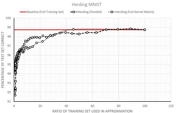
4.6 Herding for Sparse Approximation . . . 73
4.6.1 Rates of Convergence for Herding . . . 74
4.6.2 Computational Analysis of Herding . . . 75
4.6.3 Parallel Extension . . . 75
4.6.4 Discriminative Herding for Approximating Rule 4.2 . . . 76
4.6.5 Comparisons with Previous Work . . . 76
4.6.6 Comparing Herding to Sparse SVM Solvers . . . 76
4.6.7 Sparsity Inducing Objectives versus Sparsity Inducing Algo-rithms . . . 77
4.7 Conclusion . . . 78
Appendix to Chapter 4 . . . 79
4.8 Proof of Concept Experiment . . . 79
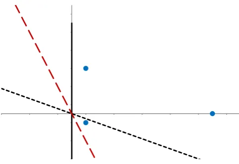
4.9 Long and Servedio Example . . . 80
4.10 Proof of Theorem 4.1 . . . 81
4.11 PAC-Bayesian Bounds for Linear Loss . . . 81
4.12 Proof of Theorem 4.6 . . . 85
4.13 Comparison with Makovoz’s Theorem . . . 86
4.14 Proof of Lemma 4.12 and Theorem 4.13 . . . 87
4.15 Proof of Theorem 4.14 . . . 89
4.16 Proof of Theorem 4.15 . . . 89
4.17 Proof of Theorem 4.16 . . . 89
4.18 Proof of Theorem 4.17 . . . 90
5. Feature Learning via Transitions . . . 91
5.1 Notation and Preliminaries . . . 92
5.2 Supervised Feature Learning . . . 92
5.2.1 Link to Deficiency . . . 93
5.3 Unsupervised Feature Learning . . . 94
5.3.1 Surrogate Approaches Motivated by Theorem 5.2 . . . 95
5.3.2 Rate Distortion Theory . . . 97
5.3.3 Hierarchical Learning of Features . . . 99
5.4 Illustrations . . . 100
5.5 Conclusion . . . 101
Appendix to Chapter 5 . . . 103
5.6 Proof of Theorem 5.1 . . . 103
5.7 Proof of Theorem 5.4 . . . 103
5.8 Proof of Theorem 5.7 . . . 104
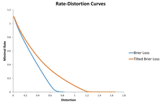
5.9 Tilted Loss Functions . . . 104
5.10 The Information Bottleneck/ Clustering with Bregman Divergences . . 106
6. Conclusion . . . 109
Appendix 111 A. PAC-Bayesian Generalization Bounds . . . 113
A.1 Information Exponential Inequality and Annealed Loss . . . 114
A.2 The Main Theorems . . . 115
A.3 Replication and Rates . . . 117
A.4 Relationship to Union Bounds . . . 118
A.5 Bounds for Bounded Losses . . . 118
A.6 The ERM Principle . . . 120
2.1 Plot of super prediction set and its lower boundary for log loss. . . 14
2.2 Construction of canonical coordinates for log loss. . . 15
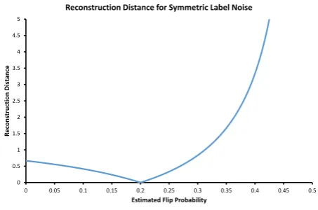
3.1 Plot of kRσ−Rσ0k1 forσ = 0.2. kRσ−Rσ0k1 is a measure of how far apart two corruptions are. . . 46
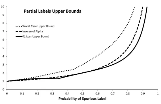
3.2 Upper and lower bounds for the problem of learning from partial labels. 49 4.1 Experiment on the MNIST data set highlighting herding’s ability to compress data sets. . . 79
4.2 Long and Servedio’s example highlighting the non-robustness to label noise of hinge loss minimization. . . 80
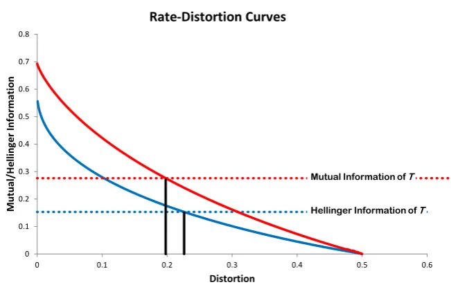
5.1 Rate-Distortion plots using mutual information showing the perfor-mance of a channel for two different loss functions. . . 98
5.2 Generalized Rate-Distortion Plots providing lower bounds on the qual-ity of features via mutual and Hellinger information. . . 99
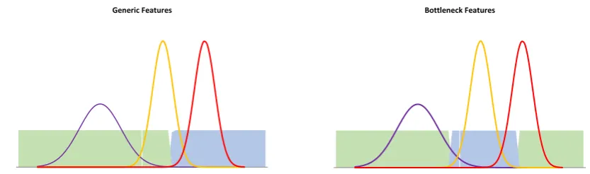
5.3 Loss Sensitive versus Loss Insensitive Features. . . 101
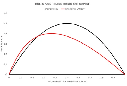
5.4 Breir and Tilted Breir entropies. . . 105
Introduction
The Problem:The massive reduction in the cost of collecting, storing, trans-porting and processing data has meant an increasing need for tools to make sense of it. Unfortunately, the deployment of modern machine learning tools is more akin to a craft than an engineering discipline: the inference problems to be solved are often under-specified or ill-posed and the available tools are often adhoc - lack-ing generality, transparency, usability and interoperability. Our premise is that the root cause of these difficulties is a lack of a clear conceptual basis for machine learning as an information engineering discipline.
- Robert C. Williamson,Reconceiving Machine Learning
This thesis presents part of the required conceptual basis. Machine learning methods afford means to automate the discovery of relationships in data sets. A relationship between quantities X andY allows the prediction of one quantity given information of the other. It is these relations that we make the central object of study. We call these relationstransitions.
Definition 1.1. Atransitionfrom a set X to a set Y is a function T : X→ P(Y), from X into the probability distributions on Y.
Intuitively, a transition T summarizes the uncertainty in predicting the quantity
Y given the observation of a quantity X. Many concepts in machine learning; such as forecasts, probabilistic models, experiments, algorithms, conditional probabilities, randomized decision rules, communication channels and so on, canallbe understood abstractly as transitions. Transitions therefore will serve as a guiding light.
1
.
1
Outline of the Thesis
Chapter one provides the abstract language underpinning the rest of the thesis. U-tilizing tools from statistical decision theory, it shows how to defineandcomparethe information content in transitions. We do this through the notion ofrisk. The risk has been shown previously to include a large number of information functions present in the literature, including the often used mutual information and KL-divergence [62; 105]. While most of the material is review, its presentation is greatly streamlined through the focus on transitions. Its novel contributions include; a generalization of the data processing theorem of information theory [46] (theorem 2.28) and means to calculate deficiency distances [85] via linear programming (lemma 2.35).
Chapter two considers the problem of learning from corrupted data. In the nor-mal theoretical analysis of supervised learning algorithms, it is assumed the decision maker has access to cleandata, that their observations are from the pattern they are expected to predict [25]. In the real world this is usually not the case, data is normal-ly corrupted and real world data sets are amalgamations of data of variable type and quality. Understanding how tolearn from andcompare different corrupted data sets is therefore a problem of great practical importance. This chapter provides a simple correction to ERM style algorithms (theorem 3.2) that facilitates learning from a large class of corrupted data sets. Furthermore, upper and lower bounds for this problem (theorems 3.4 and 3.15) are presented. These bounds allow thecomparisonof different corrupted data sets.
Chapter three focuses on one particular corrupted learning problem, namely the learning of classifiers under symmetric label noise. A conceptually simple, easily parallelized and robust classification algorithm is motivated and analysed. This al-gorithm highlights the practical benefits thatfocusingon transitions can bring.
Finally, chapter four utilizes transitions in the study of feature learning methods. Study began in this direction to take up a challenge posed by Yann LeCun to the ma-chine learning theory community at the Conference on Learning Theory 2013 [87]. It presents means to quantify the quality of learnt features independently of the su-pervised learning algorithm the features are used in. It is an attempt to provide a conceptual foundation of unsupervised, "deep" methods for the automated learning of features. Theorems 5.2 and 5.4characterizewhen it is possible to learn generical-ly good features from unlabelled data. Theorem 5.5 motivates several unsupervised learning algorithms as surrogate approaches to minimizing the quantities in theorem 5.2. Furthermore, we explore supervised feature learning algorithms and show their relationship to risks and deficiency presented in chapter one.
Decision Theory, Transitions and
Experiments
Science
The intellectual and practical activity encompassing the systematic study of the structure and behaviour of the physical and natural world through observation and experiment.
The scientific process is a means for turning the results of experiments into knowl-edge about the world in which we live. Much recent research effort has been directed toward automating the scientific process. To do this, one needs to formulate the sci-entific process in a precise mathematical language. This chapter specifies one such language. What is presented here is hardly new. The material leans much on great thinkers of times past [23; 53; 85; 125; 126] as well as more modern contributions [52; 67; 86; 105; 117]. It serves as the conceptual foundation for this thesis. The pre-sentation is abstract; this is intentional. By laying bare thebasiclanguage, we remove the distraction that focusing onspecificproblems brings, and we expose the common elements all representable by transitions.
2
.
1
Basic Notation
We require the following notation. LetR+ be the set of non-negative real numbers. Let YX be the set of functions with domain X and rangeY. For a set X define the functions idX(x) =x, and1X(x) =1. For a function f ∈RX×Y andy∈Y, we denote the partial function f(−,y) ∈ RX, with f(−,y)(x) = f(x,y), with similar notation for fixing the first argument. We denote thedual space of RX, the set of linear maps
2
.
2
A Simple, Motivating Example
Consider the problem faced by a scientist in a laboratory. In front of them is a beaker, containing one of a number of possible substances. Available to them are a myriad of experiments that can be performed to identify the unknown substance. The sci-entist could attempt to ignite it, mix a bit of it with some other known substance and see what happens, x-ray a sample, throw some of it at high velocity toward an oncoming beam of electrons and so on. Due to time and budget constraints, only a limited number of experiments can be performed to ascertain the substances true identity. Therefore the scientist should focus their effort on the "most informative" experiments. Of course, what is informative is dependent on how the substance is to be used. For example, if the scientist wishes to sprinkle some of it on their food to enhance its flavour, misidentifying arsenic as table salt is a very bad idea. However, if they want to sprinkle it on the snails in their garden, this distinction is less important. The focus of this chapter is the abstract formulation of this problem. We present a language for making decisions under uncertainty, a definition of an experiment and finally means to quantify the information contained in an experiment.
2
.
3
The General Decision Problem
We consider the problem of how a decision maker, or scientist, uses observations from experiments to inform their decisions. LetΘbe a set of possible values of some unknown quantity, and A the set of actions available to the decision maker. The consequence of an action is measured by a loss functionL :Θ×A→R. A negative loss represents a gain to the decision maker. In light of our previous example, Θare the possible substances that could be in the beaker, A is what the decision maker can do with the substance (eat it, put it on snails and so on), and L measures the consequence of an action to the scientist (L(arsenic, eat)should be high). The norm of a loss function is given by its largest possible consequence (positive or negative), kLk∞ =maxθ,a|L(θ,a)|.
To avoid measure theoretic technicalities, we assume Θ to be finite and A to be closed, compact, set with L a continuous function. This ensures that infima of all the quantities defined can be replaced by minima. Ultimately the methods suggested in this thesis will (hopefully) run on a computer, meaning all real world objects we wish to simulate need to be approximated by elements of a finite set. For those that feel this restriction places severe limitations on the theory developed here, we point out that all the following can be proven in the more general setting, at the cost of a more technical presentation. For example the reader is directed to theorem 6.2.12 of Torgersen [117], for direction on how results for finiteΘcan be extended to those for infiniteΘ.
to their limited information concerning the phenomena, the decision maker does not know the exact value of θ. They may have a vague idea of whichθ are more or less
likely to occur. This uncertainty is represented by a probability distribution.
Definition 2.1. Aprobability distributionon a set X is an element of(RX)∗, i.e. a linear functionEP :RX →R, such that:
1. EP(1X) =1.
2. If f(x)≤g(x), ∀x ∈X thenEP(f)≤EP(g).
The linear function EP is called an expectation. For a large class of general topo-logical spaces, this definition is equivalent to the usual one in terms of measures on sigma algebras 1 [79]. Focusing on the expectation operator rather than its repre-sentation via measures on sigma algebras and Lebesgue integrals provides means to "abstract away" the sample space. The function f can be thought of as a gamble taken by the decision maker, with f(x) being the loss incurred if the outcome x is observed. The expectationEP(f)is the total loss assigned to f by the decision maker. The gamble f is preferred to the gamble gif it has lower expected loss. Expectation is
oneway of ordering gambles. The first condition can be seen as a normalization, loss 1 is assigned to the constant gamble1X. The second condition can be seen as the sen-sible requirement that if f always offers lower loss thang, the decision maker always prefers f to g. If necessary, we use the notationEx∼Pf(x)to make clear what quan-tity we are taking expectations over. We drop the subscript when this is clear from context. We also make use of the following infix notation to denote expectations,
Ex∼Pf(x) =hP,fiX.
This notation for expectations is not standard, angled brackets are normally reserved to denote inner products. For finite spaces expectations are exactlyinner products. We continue with both notations where appropriate. In particular the infix notation makes it easier to see connections to concepts in functional analysis, such as adjoint operators, that are so key to the ideas presented in chapter 3.
Denote the set of probability distributions onXbyP(X), and the set of un-normalized distributions (those linear functions for which property (1) in definition 2.1 does not hold) by P+(X). This is a convex subset of (RX)∗. For x ∈ X, denote the point mass distribution onxbyδx. A probability distributionP∈P(Θ)facilitates the deci-sion making process. The decideci-sion maker acts by choosing the action with minimum expected loss,
arg min a∈A
Eθ∼PL(θ,a).
The key question iswhich distribution to use. To discoverthis distribution, the deci-sion maker is guided by experiments. Before we discuss the language for defining
1The key is to identify sets with their indicator functions. P∈(RX)∗defines a measure viaP(C):=
and ordering experiments, we first focus on how to construct suitable loss function-s. We show that the essential properties of a loss needed for the decision making process are encoded in its correspondingentropy,
L(P) =min
a∈AEθ∼PL(θ,a).
We show that each entropy defines acanonical loss function. We also show that for the sake of developing theory, one only need work withcanonicallosses.
Aside: Loss versus Regret
It is quite natural in decision theory to work with the regret,
∆L(P,a) =Eθ∼PL(θ,a)−min
a0∈AEθ∼PL(θ,a 0),
which measures the excess loss of the decision makers action versus the loss of the optimal action if they knewP. Here we focus on loss, elsewhere we focus on regret.
2
.
4
Representing Loss Functions
In this section we make heavy use of the infix notation for expectations, as well as partial functions. In its partial form, a loss provides a mapping partialL : A → RΘ with,
partialL(a) = L(−,a)∈RΘ.
In words, when the decision maker chooses an action a, they specify a function that takes the unknown and returns the loss incurred by the decision maker. Choosing an action is then equivalent to picking a partial loss function. In our notation,
Eθ∼PL(θ,a) =hP,L(−,a)iΘ.
In many statistical problems, it is natural for the space of actions Ato be the set of distributions over unknownsP(Θ).
Definition 2.2. A loss L:Θ×P(Θ)→Risproperif for all distributions P ∈P(Θ),
P∈arg min Q∈P(Θ)
hP,L(−,Q)iΘ.
It isstrictly properif P is theuniqueminimizer.
Intuitively, a proper loss takes a prediction Q ∈ P(Θ), and then penalizes the decision maker according to how much weight their prediction assigned to the un-known θ. Intuitively properness ensures that if the decision maker knows P, then
[7; 31; 52; 52; 64; 67; 106; 133].
As will be shown, all ”sensible" losses are essentially re-parametrized proper losses. We show how toconstructproper losses from their entropies. Furthermore, we show how to render any proper loss convex through a canonical re-parametrization. This allows the use of tools from convex analysis [26; 90] to aid in calculating optimal actions.
2.4.1 Entropy from Loss
Rather than working with probability distributions, we take the route of Williamson in [129] and work with un-normalized distributions. For any loss function L, define theentropy L:P+(Θ)→R,
L(µ) =min
a∈Ahµ,L(−,a)iΘ.
L(P) measures the uncertainty of the optimal action for the distribution P. The entropy is also called anuncertainty function, aBayes riskor asupport function[53; 105; 129]. It is concave and 1-homogeneous.
Definition 2.3. A function f :P+(Θ)→Ris 1-homogeneous if for all x∈ P+(Θ)and for
allλ>0,
f(λx) =λf(x).
2.4.2 Loss from Entropy
All loss functions give rise to an entropy. Conversely, the entropy encodes much information of its associated loss through its super-gradients, which include all the
Bayesactions for the underlying loss.
Bayes Actions and Super-gradients
For any distributionP, define theBayes actionsfor Pas the set of minimizers,
AP =arg min a∈A
hP,L(−,a)i.
For anyaP ∈ AP we haveL(P) =hP,L(−,aP)i.
Definition 2.4 (Super-gradient of a concave function [90]). Let f : P+(Θ) → Rbe a concave function. v∈RΘ is asuper-gradientof f at the point x if for all y ∈P+(Θ),
hy−x,vi+ f(x)≥ f(y).
Denote the set of all super-gradients at a pointxby∂f(x), and the set of all
the same as regular gradients [90]. 1-homogeneous functions afford a very simple representation via their super-gradients.
Theorem 2.5(Generalized Euler’s Homogeneous Function Theorem [51]). Let f :P+(Θ)→Rbe a concave 1-homogeneous function. Then for all x and for all v∈∂f(x),
f(x) =hx,vi.
Furthermore, v∈ ∂f(x) =⇒ v∈∂f(λx)for allλ>0.
We include a simple proof of this theorem for completeness.
Proof. Firstly, for allx and allλ>0,
hλx−x,vi+ f(x)≥λf(x),
which follows directly from the definition of a super-gradient atxand the 1-homogeneity of f. Re-arranging yields, (1−λ)(f(x)− hx,vi) ≥ 0. Letting λ → 0+ yields
f(x)≥ hx,vi. Similarly, for allxand allλ>0,
hx−λx,vi+λf(x)≥ f(x),
which follows directly from the definition of a super-gradient at λx and the
1-homogeneity of f. Re-arranging yields,(1−λ)(f(x)− hx,vi)≤ 0. Letting λ → 0+
yields f(x)≤ hx,vi, therefore f(x) =hx,vi.
To prove the second claim, we have for allyandλ>0,
hy−x,vi+ f(x)≥ f(y)
hλy−λx,vi+ f(λx)≥ f(λy),
where the first line is by definition, and the second is by 1-homogeneity. As y is arbitrary, the claim is proved.
This theorem provides a corollary, that shows the super-gradients of a 1-homogeneous function have a property similar to properness.
Corollary 2.6. Let f : P+(Θ) → R be a concave 1-homogeneous function. Then for all x,y∈P+(Θ)and for all v
x ∈∂f(x), vy∈ ∂f(y),
hx,vyi ≥ hx,vxi.
We now show that the partial loss of a Bayes action is a super-gradient of L.
Proof. ForaP ∈ AP we have for allµ∈P+(Θ),
hµ−P,L(−,aP)i+L(P) =hµ,L(−,aP)i ≥min
a∈Ahµ,L(−,a)i= L(µ). Hence L(−,aP)∈∂L(P). For the converse, if L(−,aP)∈∂L(P)then,
L(P) =hP,L(−,aP)i=min
a∈AhP,L(−,a)i, meaning ais Bayes.
Therefore, once inadmissible actions are discarded, we can identify a loss with a subset of ∂L. Rather than working with a subset ∂L, it is advantageous to consider
allof ∂L.
Definition 2.8 (Canonical Loss). Let L : P+(Θ) → R be a concave, 1-homogeneous function. Then itscanonical loss,L:Θ×∂L→Ris given by,L(θ,`) =`(θ).
As will be shown, canonical losses can always be convexified. Furthermore, they maintain all of the properties ofLneeded for assessing the quality of decisions.
The Bayes Super Prediction Set
The process ofcanonisinga loss, i.e. going from,
L→L→ L,
can createextrapartial losses/actions that were not originally available to the decision maker under L. However, they gain no benefit from these extra actions. From any entropy define theBayes super prediction set,
SL:= n`∈RΘ :hµ,`i ≥L(µ), ∀µ∈ RΘ+
o
.
By the definition,
min
a∈AhP,L(−,a)i=min`∈SL
hP,`i, ∀P∈P(Θ).
The Bayes super prediction set is precisely those partial losses that the decision maker need not use over the actions available to them, no matter the distribution P. The super prediction set is convex. Furthermore, the Bayes actions for L are the lower boundary of the super prediction set.
Lemma 2.9. Let L : P+(Θ) → R be a concave, 1-homogeneous function. Then` ∈
∂L if
and only if,
hµ,`i ≥ L(µ), ∀µ∈P+(Θ),
The proof is a straightforward application of 1-homogeneity and super-gradients.
Admissible Actions
Bayes actions are one notion of optimal action. Admissibility affords another.
Definition 2.10. Let L be a loss. An action a isadmissibleif there does not exist an action a∗ such that,
L(θ,a∗)≤L(θ,a), ∀θ ∈Θ,
with strict inequality for at least oneθ.
Intuitively, an action is admissible if there is no other action that is obviously better. Bayesian actions are optimal if the decision maker has knowledge about the unknown, given in the form of a probability distribution. Interestingly, the class of admissible and Bayesian actions are the same for many loss functions.
Theorem 2.11(Complete Class Theorem [24; 126] ). Let L be a loss such thatim(partialL) is a convex subset ofRΘ. Then the set of Bayes actions for L is in 1-1 correspondence with the set of admissible actions for L.
If the decision maker is allowed to usedrandomizedactions, i.e. distributions over
Awith L(θ,Q) =Ea∼QL(θ,a), then all admissible actions are Bayesian actions.
Proper Losses
Using the canonical loss allows the construction of proper losses from entropies.
Lemma 2.12 (Loss from Entropy). Let L : P+(Θ) → R be a concave, 1-homogeneous function and let∇L : P+(Θ) → RΘ be a super-gradient function, ∇L(µ) ∈ ∂L(µ), ∀µ.
Then,
L(θ,Q) =L(θ,∇L(Q)),
is a proper loss. Furthermore if L is strictly concave then L is strictly proper.
Regret for Proper Losses
Recall the notion of regret,
∆L(P,a) =Eθ∼PL(θ,a)−min
a0∈AEθ∼PL(θ,a 0).
For proper losses, the regret takes on the particularly elegant form,
∆L(P,Q) =Eθ∼P[L(θ,Q)−L(θ,P)] =hP,∇L(Q)− ∇L(P)i.
The regret for a proper loss is also equal to the Bregman divergence between Pand
Q. We have,
L(Q) +hP−Q,∇L(Q)i −L(P)
| {z }
Bregman divergence induced byL
where we have used the fact that L(Q) =hQ,∇L(Q)i.
2.4.3 Convexification of Losses in Canonical Form
The preceding shows how toconstructlosses, we begin with a convex 1-homogeneous function and then take super-gradients. Focus now turns to their convexification. Once convexified, the decision maker gains access to the large and ever growing lit-erature on the minimization of convex functions to aid in the calculation of optimal actions. The development here closely follows that in [52], which focused on proper losses. Working with canonical versus proper losses streamlines the development. For example, for some proper losses lemma 2.14 fails to hold, while it does hold for all canonical losses. Furthermore, our result on convexification of canonical losses (theorem 2.16), is to the best of our knowledge novel.
Recall 1Θ ∈ RΘ is the function that always returns 1, and define 1⊥Θ to be its or-thogonal complement inRΘ, i.e. the functionsv ∈RΘ with,
h1Θ,vi=
∑
z∈Θ
v(z) =0.
Define,
ΓL= {(γ,v)∈R×1⊥Θ :γ1Θ+v∈∂L}.
Lemma 2.13. Let(γ,v)∈ΓL. Thenγis uniquely determined by v.
Proof. Fixv and suppose there exists γ1 andγ2 with γ1 < γ2 andγ11Θ+v,γ21Θ+
v∈ ∂L. By assumption,γ21Θ+vis Bayes for some distribution P. But,
hP,γ11Θ+vi=γ1+hP,vi<γ2+hP,vi=hP,γ21Θ+vi,
a contradiction.
Thus we lose nothing by working with projections of losses onto 1⊥Θ. Geometri-cally, we have the following sequence of maps,
∂L
partialL //
RΘ proj1⊥Θ //
1⊥Θ,
with proj1⊥
Θ the projection onto 1 ⊥
Θ. Lemma 2.13 shows that proj1⊥Θ ◦partialL is
in-vertible. Define,
ˆ
ΓL =im(proj1⊥
Θ ◦partialL)⊆1 ⊥
Θ.
By lemma 2.13 ˆΓLis in 1-1 correspondence with∂L.
Proof. To show ˆΓL is convex, we are required to show that for all `1,`2 ∈ ∂L and all λ∈[0, 1]there is a constantγsuch that,
λ`1+ (1−λ)`2−γ1Θ ∈ ∂L.
By lemma 2.9, this is equivalent to,
λhP,`1i+ (1−λ)hP,`2i −L(P)
| {z }
γ(P)
−γ=γ(P)−γ≥0, ∀P∈P(Θ),
with equality holding for one P. Letγ∗ = minPγ(P), with P∗ the distribution that
achieves the minimum. Then,
λhP,`1i+ (1−λ)hP,`2i −γ∗ ≥ L(P), ∀P∈P(Θ),
with equality forP∗. Therefore by lemma 2.9, λ`1+ (1−λ)`2+γ∗1Θ ∈∂L.
Define the functionΨ: ˆΓL→Rsuch that,
v+Ψ(v)1Θ ∈ ∂L.
By lemma 2.13,Ψis well defined.
Lemma 2.15. Ψis a convex function.
Proof. Let v1,v2 ∈ΓˆLwithvλ =λv1+ (1−λ)v2. Let their partial losses be,
`1 =v1+Ψ(v1)1Θ
`2 =v2+Ψ(v2)1Θ
`λ =λv1+ (1−λ)v2+Ψ(λv1+ (1−λ)v2)1Θ,
respectively. By assumption, for allλ∈ [0, 1]there exists a distributionPλ such that,
hPλ,`λi ≤ hPλ,`i, ∀`∈ ∂L.
Assume there is aλ∗ such that,
λ∗Ψ(v1) + (1−λ∗)Ψ(v2)<Ψ(λ∗v1+ (1−λ∗)v2). But then,
hPλ∗,λ ∗`
1+ (1−λ∗)`2i<hPλ∗,`λ∗i,
a contradiction.
Theorem 2.16(Representation of Canonical Losses). Let L:P+(Θ)→Rbe a concave, 1-homogeneous function. Then its canonical lossL can be represented asL : Θ×C → R,
with C⊆1⊥Θ a convex set and,
L(θ,v) =v(θ) +Ψ(v),
for a convex functionΨ.
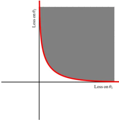
2.4.4 Example: Binary Decisions and Log Loss
For this example, takeΘ={−1, 1}, with lossL(−,p) = (−log(1−p),−log(p))for
p ∈ (0, 1), where pis the probability that θ =1. We plot this loss in 2.1. The partial
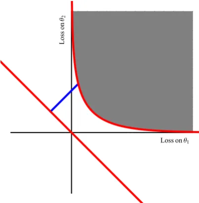
losses are given by the red curve, the super prediction set in grey. The loss on neg-atives is plotted on the x-axis. In figure 2.2 we show geometrically how to produce canonical coordinates.
For canonical coordinates, We seek to decompose L(−,p) = γ1v+γ21Θ, where
v = −12,12
. Here we have projected p = 0.8 onto 1⊥Θ. The length of the blue line is related to Ψ(γ1). Solving forγ0andγ1in terms of pgives,
γ1=log
p
1−p
andγ2 = 1 2log
1
p(1−p)
.
This equation can be easily solved for p, giving,
p= exp(γ1)
1+exp(γ1)
andγ2=Ψ(γ1) =log(1+eγ1)−
γ1 2 .
The above relationship betweenpandγ1is exactly that given by thecanonical linkfor log loss [104]. Finally for log loss,
L(−,γ) =γv+ (log(1+eγ)−γ
2)1Θ.
This yields,
L(y,γ) =log 1+e−yγ,
the usual form of logistic loss.
2.4.5 Misclassification and Linear Loss
For any observation space define themisclassificationlossL01 :Θ×Θ→R,
Loss onθ1
Loss
on
[image:30.595.182.377.112.312.2]θ2
Fig. 2.1: Plot of super prediction set and its lower boundary for log loss, see text.
In words, the decision maker incurs loss 1 if their prediction is different to their observation and no loss otherwise. Allowing randomized actions giveslinearloss,
Llinear(θ,Q) =Eθ0∼QL01(θ,θ0).
In canonical form, linear loss can be written as L(−,v) = v+ |Θ|Θ|−|11Θ. By theorem 2.16, linear loss is therefore the primitive loss, as it is the linear term in all other canonical losses. We will see in chapter 4, that linear loss provides means to learn classifiers.
2
.
5
Experiments
Recall that the decision maker chooses their actions by minimizing their expected loss,
arg min a∈A
Eθ∼PL(θ,a).
The key question is which distribution to use. To discover this distribution, the de-cision maker is guided by experiments. Let Z be a finite set of possible outcomes of an experiment. The outcome of the experiment, z ∈ Z, is assumed related to the unknown, certain outcomes are more strongly linked to certain values ofθ. The
relationship between the unknown and the outcome of the experiment is modelled by atransition.
2.5.1 Transitions and their Algebra
Loss onθ1
Loss
on
[image:31.595.215.417.112.318.2]θ2
Fig. 2.2: Construction of canonical coordinates for log loss, see text.
Denote the set of all transitions from X toY byT(X,Y). Transitions (or Markov kernels), constitute a modern approach to conditional probability [36; 39; 85; 117]. The distributionT(x)is how the decision maker summarizes their uncertainty about
Yif the true value of Xisx. Every functionφ∈YX defines a transition with,
hφ(x),fiY = f(φ(x)), ∀f ∈RY.
Such a transition is called deterministic. Transitions can also be thought of as dual mappings,T:(RX)∗ →(RY)∗. We define,
hT(α),fiY =hα,hT(x),fiYiX, ∀f ∈RY, ∀α∈ (RX)∗.
The function T∗(f)(x) =hT(x),fiY is thepullback of f byT. Formally, the operator
T∗ is the adjoint or transposeof T. Transitions can be composed. For transitions T ∈
T(X,Y)andS∈T(Y,Z)we can defineS◦T∈T(X,Z)with,
hS◦T(x),fiZ =hT(x),hS(y),fiZiY, ∀f ∈RZ.
In usual notation, this is just iterated expectation,
hS◦T(x),fiZ=Ey∼T(x)Ez∼S(y)f(z).
Intuitively, this can be seen as "marginalizing" overY in the Markov chain,
X →Y→ Z.
Transitions can also be combined in parallel. For P,Q ∈ P(X), denote the product distribution byP⊗Q. IfTi ∈T(Xi,Yi),i∈[1;k], are transitions then denote,
⊗ki=1Ti ∈T(×ki=iXi,×ki=1Yi)
with ⊗k
i=1Ti(x) = T1(x1)⊗ · · · ⊗ Tk(xk). Transitions can also be replicated. For any transition T ∈ T(X,Y) we denote the replicated transition Tn ∈ T(X,Yn), n ∈ {1, 2, . . .}, with,
Tn(x) =T(x)⊗. . .T(x)
| {z }
ntimes
= T(x)n,
the n-fold product of T(x). A distribution P ∈ P(X)and a transition T ∈ T(X,Y)
can be combined into ajointdistributionPnT∈P(X×Y), with,
hPnT,fiX×Y= hP,hT(x),fxiYiX =Ex∼PEy∼T(x)f(x,y), ∀f ∈RX×Y.
Bayes theorem provides means todisintegrate[36; 111] a joint distribution PXnTX→Y into a joint distribution PYnTY→X, where PX ∈ P(X) and TX→Y ∈ T(X,Y), and
PY ∈ P(Y) and TY→X ∈ T(X,Y). Disintegration theorems hold in very general spaces, not just the cases considered here.
2.5.2 Comparing Experiments
An experimentis a transition e ∈ T(Θ,Z). We call Z the observation space of the experiment. The distribution e(θ) summarizes the decision maker’s uncertainty in
the observation when θ is the value of the unknown. After observing the results of
an experiment, the decision maker is tasked with choosing a suitable action. They do this via alearning algorithm.
Alearning algorithmis a transitionA ∈T(Z,A). A(z)summarizes the decision mak-ers uncertainty in which action to choose, given an observationz∈ Z. We define the
risk,
RL(θ,e,A) =Ez∼e(θ)Ea∼A(z)L(θ,a).
The risk measures the quality of the final action chosen by the decision maker when they use the learning algorithm A, after performing experiment e, assuming θ is
the true value of the unknown. The risk does not provide a single number for the comparison of experiments, rather it provides an entirerisk profile. To compare risks directly, the decision maker can use theBayesianormaxrisks defined as,
Rπ
L(e,A):=Eθ∼πRL(θ,e,A)andRL(e,A):=sup θ
RL(θ,e,A),
respectively. The Bayesian risk is more appropriate if the decision maker has some intuition about θ, given in the form of a prior probability distribution π. The max
These quantities allow the decision maker to comparethe usefulness of experiment, learning algorithm pairs. To compare experiments directly, we assume the decision maker uses thebestlearning algorithm. Define the minimum Bayesian risk and min-imax risk as,
Rπ
L(e):=min
A R π
L(e,A)andRL(e):=min
A RL(e,A),
respectively. The minimum Bayes risk and the minimax risk are deeply related.
Theorem 2.18. For all experiments e and loss functions L,
RL(e) = sup
π∈P(Θ) Rπ
L(e).
The proof is a simple application of the minimax theorem [82]. In light of this theorem, we focus on Bayesian risks for the remainder. All results have a minimax equivalent.
We also point out to the reader that all notions here have relative versions. For example therelative riskis defined as,
∆RL(θ,e,A) =RL(θ,e,A)−inf
a∈AL(θ,a),
which measures the risk relative to knowingθ.
Abstracting Away the Observation: Risk as Loss
Ultimately, what matters to the decision maker is not the exact details of the exper-iment and their learning algorithm. What matters is that the distribution A ◦e(θ)
places high weight on actions that are suitable forθ. We can think of risk as a loss,
RL :Θ×T(Θ,A)→R,
with RL(θ,A) = Ea∼A(θ)L(θ,a). Different experiments allow the decision maker
access to different subsets ofT(Θ,A).
Admissible and Bayesian Learning Algorithms
The optimal learning algorithm will in general depend on their prior knowledge about the unknown. Even without this knowledge, the decision maker can remove rules that are obviously not optimal.
Definition 2.19. Let e be an experiment. A learning algorithm A is admissible for e if there does not exist a learning algorithmA0 with,
with strict inequality for at least oneθ.
Intuitively, a learning algorithm is admissible if it is not obviously worse than some other learning algorithm. If the decision maker has priorπ, they can minimize
the Bayesian risk by using a Bayesian learning algorithm.
Definition 2.20. Let e be an experiment and π a prior. A learning algorithm A∗ isBayes
for(π,e)if,
A∗∈ arg min
A
Rπ
L(e,A).
Much like the case for Bayesian actions, the decision maker need only consider Bayesian learning algorithms.
Theorem 2.21 (Complete Class Theorem [126]). A learning algorithm Ais admissible for e if and only if there exists a priorπsuch thatAis Bayes for(π,e).
The above theorem says that Bayesian algorithms provide all rules that a sensible decision maker should use. Picking a particular admissible algorithm isequivalent to picking a priorπ and minimizing the Bayesian risk against that prior. While
statis-tically, admissible algorithms afford no obvious improvements, they may be hard to implement. Our language as is does not take this into account. The study of inad-missible algorithms and their risks is therefore a worthwhile endeavour.
Bayes optimal algorithms admit a simple representation. A prior π and an
exper-imente define a joint distribution on pairsΘ× Z in the obvious way. LetπZ be the
marginal distribution over the observation space, and η ∈ T(Z,Θ) be the induced
conditional distribution of unknowns given observations. Then,
Rπ
L(e) =Ez∼πZL(η(z)),
with Bayes optimal algorithm,
A∗(z):=arg min a∈A
Eθ∼η(z)L(θ,a).
We stress that this algorithm is prior dependent, ηdepends on the prior π and the
experiment T.
2.5.3 When is One Experiment Always Better than Another?
Definition 2.22. Let e∈T(Θ,Z)and e0 ∈T(Θ,Z0)be experiments. edividese0(written e |e0) if there exists a transition T∈T(Z,Z0)such that e0 =T◦e.
Intuitively, e |e0 if e0 ise with extra noiseT. We make this intuition precise with theorem 2.24. For an experimente, letTe(Θ,A)be the set of transitions fromΘto A thate divides.
Theorem 2.23. e divides e0 if and only if for all action sets A,
Te0(Θ,A)⊆Te(Θ,A).
Proof. The forward implication follows simply from the definition. For the converse, take A=Z0 and notee0 ∈T
e0(Θ,Z0). By assumption,
Te0(Θ,Z0)⊆Te(Θ,Z0).
Ase0 ∈Te0(Θ,Z0), this implies there exists aT withT◦e =e0.
The Blackwell-Sherman-Stein Theorem and Sufficiency
Theorem 2.24 (Blackwell-Sherman-Stein Theorem [24]). Let e and e0 be experiments. e |e0 if and only if for all action sets, loss functions and priors,
Rπ
L(e)≤ RπL(e0).
We prove the forward implication, called the data processing theorem. The proof of the converse will come later, as a simple corollary of the randomization theorem.
Proof. For any learning algorithm A0 ∈ T(Z0,A) consider the learning algorithm A=A0◦T∈ T(Z,A). Ase0 = T◦e, it is easy to verify that,
Rπ
L(e0,A0) =RπL(T◦e,A0) =RπL(e,A0◦T) =RπL(e,A). To complete the proof take minima overAandA0.
We say e ande0 areequivalent experiments (writtene∼= e0) if bothe |e0 ande0 |e. Equivalent experiments have equivalent risks. A key notion in statistics is that of
sufficiency. A sufficient statisticis a function of the observation that loses none of the information contained in e. The Blackwell-Sherman-Stein theorem provides means to define and understand sufficiency. Identifying and exploiting sufficient statistics allows the decision maker to compress the information contained in the observation, without losing information.
By the Blackwell-Sherman-Stein theorem, sufficient statistics maintain all infor-mation in the observation, under the assumption the decision maker uses the best learning algorithm for each experiment.
For any set Θ of unknowns there is a most informative and a least informative ex-periment. Recall the identity function idΘ, idΘ(θ) = θ. For any experiment e, we
havee◦idΘ =e. Therefore, idΘ divides any experiment. Intuitively, idΘprovides the decision maker theexactvalue ofθ. This experiment has risk,
Rπ
L(idΘ) =Eθ∼πmin
a∈A L(θ,a).
For any set X, define the terminal transition •X ∈ {1}X with •
X(x) = 1 for all X. Intuitively this transition throws away all information about X. Much like the iden-tity transition divides every experiment, the terminal transition is divided by every experiment. For all experimentse,•Θ =•Z◦e. This experiment has risk,
Rπ
L(•Θ) =L(π). By the data processing theorem,
Rπ
L(idΘ)≤ RπL(e)≤ RπL(•Θ).
Relationship to the Standard Data Processing Theorem
Definition 2.26. Let f :R+→Rbe a convex function with f(1) =0. For all distributions
P,Q∈P(Z)the f-divergencebetween P and Q is,
Df(P,Q) =hP,f
dQ dP
i,
if Q is absolutely continuous with respect to P and is undefined otherwise.
f-divergences provide one means of measuring thedissimilarityof two probability distributions. They include many standard measures of dissimilarity, including the KL-divergence, the Hellinger divergence and variational distance [2; 48]. The stan-dard data processing theorem states that for all setsZ, ˜Z, all transitionsT∈T(Z, ˜Z), all distributionsP,Q∈P(Z)and all f-divergences,
Df(T(P),T(Q))≤Df(P,Q).
Intuitively, adding noise always makes it harder to distinguishPandQ. This theorem is actually theorem 2.24 in disguise. The pair P,Q ∈ P(Z) define a transition e ∈
T({−1, 1},Z), withe(1) =Pande(−1) =Q.
e ∈T({−1, 1},Z),
Rπ
L(•Θ)− RπL(e) =L(π)− RLπ(e) =Df(e(−1),e(1)).
The data processing theorem for f-divergences follows directly from our data processing theorem. In [62] this correspondence is developed further to create
multi-f-divergences. These results highlight the foundational role played by the Bayesian risk.
Digression: Generalised Data Processing Theorems
Key to the proof of the data processing theorem is the insight that ife |e0 then,
Te0(Θ,A)⊆Te(Θ,A).
Intuitively, this means more learning algorithms are available to the decision maker after performing the experiment ethane0. This suggests another means to construct quantities that satisfy data processing theorems.
Theorem 2.28. Letψ:T(Θ,A)→Rand define the information measure,
Iψ(e) = min
A∈Te(Θ,A)
ψ(A).
If e|e0then Iψ(e)≤ Iψ(e0).
Proof. Ife |e0 thenTe0(Θ,A)⊆Te(Θ,A). Therefore,
min
A∈Te(Θ,A)
ψ(A)≤ min
A0∈T
e0(Θ,A)
ψ(A0).
We recover the usual data processing theorem by taking,
ψ(A) =Eθ∼πEa∼A(θ)L(θ,A).
Remarkably, the proof of theorem 2.28 makes no reference to expected risks, transi-tions, or even probability distributions! Much recent work has been directed toward characterizing functions that satisfy a data processing theorem [10; 49; 71]. Invariably, these approaches "cook the books", adding extra constraints until KL-divergence and mutual information are discovered to be the only such functions, and the standard data processing theorem of information theory is recovered [46].
of [75]). In the emerging fields of non-commutative probability [42; 124], a field with close ties to quantum theory, the commutative algebra of functions is replaced with general non commuting algebras. All these different systems could potentially be used in place of probability. The generality of theorem 2.28 would seem to indicate that such a theorem will excess in these other systems.
Deficiency and Quantitative Data Processing Theorems
The converse of the Blackwell-Sherman-Stein theorem states that ifedoesnotdivide
e0 then there is a loss function and prior that renderse0 more useful. Furthermore, if
e0 does not divideethen there is a loss function and prior that rendersemore useful. The gap in risks is quantified by thedeficiency.
Definition 2.29. Let P,Q ∈ P(Z)be distributions. The variational distance between P and Q is,
V(P,Q):= sup f∈[0,1]Z
|EP(f)−EQ(f)|.
Intuitively, variational distance is the maximum difference in assigned loss when making decisions via P or Q. The variational distance is a metric on probability distributions. It is an f-divergence with f(x) = |x−1| [2; 48]. This means the variational divergence satisfies a data processing inequality, for all transitions T ∈
T(Z,Z0),
V(T(P),T(Q))≤V(P,Q).
Definition 2.30. Let e ∈ T(Θ,Z) and e0 ∈ T(Θ,Z0) be experiments. The directed
deficiencyfrom e to e0 is,
ξπ(e,e0):= min
T∈T(Z,Z0)Eθ∼πV(T◦e(θ),e 0(
θ)).
The directed deficiency provides means to quantify how close eis to dividing e0.
ξπ(e,e0) =0 for all priors if and only ife |e0. Thedeficiencyis defined as,
Ξπ(e,e0):=max{
ξπ(e,e0),ξπ(e0,e)}.
Deficiency measures how close to equivalenceeande0 are. Ξπ(e,e0) =0 for all priors
if and only if e ∼= e0. The directed deficiency provides a quantitative version of the Blackwell-Sherman-Stein theorem.
Theorem 2.31(Randomization Theorem [85]). Fixe >0and a prior π. Let e and e0 be
experiments. Then,
Rπ
L(e)≤ RπL(e0) +ekLk∞
for all action sets and loss functions, if and only ifξπ(e,e0)≤e.
Proof. We begin with the reverse implication. Asξπ(e,e0)≤ e, there exists a transition
T ∈T(Z,Z0)such that,
Eθ∼πV(T◦e(θ),e 0(
θ))≤e.
Now fix a learning algorithm A0 ∈ T(Z0,A), and consider A = A0◦T as in the diagram below.
Θ
e
e0
Z
T //Z
0 A0 //AWe have,
Rπ
L(e,A)− RπL(e0,A0) =Eθ∼π h
Ea∼A◦e(θ)L(θ,a)−Ea∼A0◦e0(θ)L(θ,a) i
≤Eθ∼πV(A ◦e(θ),A 0◦e0(
θ))kLk∞
=Eθ∼πV(A
0◦T◦e(
θ),A0◦e0(θ))kLk∞
≤Eθ∼πV(T◦e(θ),e 0(
θ))kLk∞
≤ekLk∞
where the first line follows from the definition of the Bayesian risk, the second fol-lows from the definition of the variational distance, the third from the definition of A, the fourth as variational distance is an f-divergence and therefore satisfies a data processing inequality and finally from our assumptions onT. The proof is completed by taking a minimum over A0 andA.
For the forward implication, first fix a set of actions A and a learning algorithm A0 ∈T(Z0,A)and define the function,
φ(L,A) =RπL(e,A)− RπL(e0,A0)−ekLk∞.
Note thatφis affine in Aand concave in L. By the conditions in the theorem,
sup L
min
A φ(L,A)≤0.
By the minimax theorem [82] or strong convex duality [90], there exists a saddle point
(L∗,A∗)with,
φ(L∗,A∗) =min
A supL φ(L,A) =supL minA φ(L,A)≤0.
This implies,
Rπ
L(e,A∗)≤ RπL(e0,A0) +ekLk∞, ∀L.
This means Eθ∼πV(A∗◦e(θ),A0◦e0(θ)) ≤ e, from the definition of variational
A=Z0 andA0 =idZ0. The transitionT is then given byA∗.
The proof of the reverse implication of the Blackwell-Sherman-Stein theorem can be recovered by setting e = 0. The randomization theorem shows there is a deep
connection between differences of risks and deficiency. The following theorem makes this connection precise.
Theorem 2.32. Let e and e0 be experiments. For all priorsπ,
Ξπ(e,e0) = sup
L:kLk∞6=0 |Rπ
L(e)− RπL(e0)| kLk∞ .
For the proof we require the following simple lemma.
Lemma 2.33. For x,y∈Rif∀e∈R, x ≤e⇔y≤ethen x =y.
Proof. Suppose that x 6= y and without loss of generality assume that x < y. Set
e= x+2y. Thenx ≤eandy> e, which implies the contrapositive.
We now prove the theorem.
Proof. If Ξπ(e,e0) ≤
e then ξπ(e,e0) ≤ e and ξπ(e0,e) ≤ e. By the randomization
theorem,
|Rπ
L(e)− RπL(e0)|
kLk∞ ≤e, ∀L :kLk∞ 6=0. Conversely, if,
sup L:kLk∞6=0
|Rπ
L(e)− RπL(e0)| kLk∞ ≤ e, thenRπ
L(e)≤ RπL(e0) +ekLk∞ andRπL(e0)≤ RπL(e) +ekLk∞. By the randomization
theorem, this meansΞπ(e,e0) ≤
e. This combined with the above lemma completes
the proof.
The randomization theorem can be used to definequantitativeversions of concepts such as sufficiency. This was Le Cam’s original motivation for defining the quantity in [85]. Tis approximately sufficient foreifΞπ(e,T◦e)is small. Deficiency provides
a metric on experiments.
Theorem 2.34. Letπ be a prior that assigns non zero probability to each unknown. Then
Ξπ is a metric on experiments modulo equivalence.
Proof. Ξπ is obviously non-negative and symmetric. We are required to show that it
Θ e xx e 0 e00 ''
Z
T //Z
0 T0 //Z
00We have for allθ,
V(e00(θ),T0◦T◦e(θ))≤V(e00(θ),T0◦e0(θ)) +V(T0◦e0(θ),T0◦T◦e(θ))
≤V(e00(θ),T0◦e0(θ)) +V(e0(θ),T◦e(θ)),
where we have used the fact that the variational distance is a metric, followed by the data processing inequality. Averaging overπ and taking a minimum overT and T0
yields,
ξπ(e,e00)≤ξπ(e,e0) +ξπ(e0,e00).
Reversing the direction and taking maximums yields the desired result.
Calculating Deficiency
The variational distance can be calculated as thel1 distance,
V(P,Q) = 1
2z
∑
∈Z|P(z)−Q(z)|.Experiments e ∈ T(Θ,Z)can be represented by a |Z | × |Θ|column stochastic ma-trix, Tij ≥ 0 and ∑iTij = 1 for all j. Furthermore, the prior distribution π can be
represented by a vector in R|Θ|. Using these representations, the directed deficiency can be calculated via linear programming.
Lemma 2.35. Let e and e0 experiments with their stochastic matrix representation given by E and E0 respectively. Thenξπ(e,e0)can be calculated via the following linear program,
min Mij,Tij
|Z0|
∑
i=1
|Θ|
∑
j=1
Mij
subject to
Mij,Tij ≥0and
πjE
0
ij−πj[TE]ij
≤ Mij ∀i,j |Z0|
∑
i=1
Tij =1∀j,
where[TE]ij is the ij entry of TE.
Proof. The constraintsTij ≥ 0 and
|Z0|
∑
i=1
Taking the final constraint and summing overiandjyields,
|Z0|
∑
i=1
|Θ|
∑
j=1
Mij ≥
|Z0|
∑
i=1
|Θ|
∑
j=1
πjE
0
ij−πj[TE]ij
= |Θ|
∑
j=1
πj
|Z0|
∑
i=1
E
0
ij−[TE]ij
=Eθ∼πV(e0(θ),T◦e(θ)).
Equality is attained in the above if Mij = πjE
0
ij−πj[TE]ij
. Minimizing over Mand T yields an optimal solution ofξπ(e,e0).
2
.
6
Preview of the Remainder of the Thesis
While the ideas of the previous subsections originated in theoretical statistics [24; 60; 86; 117] they can be readily applied to machine learning problems. The main distinction is that statistics focuses on parametric families and loss functions of type
L:Θ×Θ→R. The goal is to accuratelyreconstruct parameters. In machine learning one is interested inpredicting the observations of the experiment well. The remainder of this thesis turns to thequantificationof the usefulness of different experiments for different prediction problems.
2.6.1 Prediction Problems
A central problem in machine learning is that of prediction. Given side information
x ∈ X, the goal of the decision maker is to correctlypredict a labely ∈Y. To do so, the decision maker specifies a function f ∈YˆX, that should have low expected loss,
E(x,y)∼P`(y,f(x)),
where ` :Y×Yˆ → R is a loss function that measures the suitability of a prediction ˆ
y. Note Y and ˆY need not be the same set, for example in conditional probability estimation ˆY =P(Y). IfP is known to the decision maker, then this is a problem of optimization. In generalPis unknown, but the decision maker has access to a sample
S ofniid draws from P,{(xi,yi)}ni=1. The sample is used as a proxy for expectation underY, and the decision maker returns the function in a restricted classF ⊆YˆX,
fS=arg min f∈F
1
n
n
∑
i=1
This is known as the empirical risk minimization (ERM) rule [122]. Of central interest are bounds on theexpected lossof the ERM rule,
ES∼PnE(x,y)∼P`(y, fS(x))
that hold regardless of the true value of P. What is unknown to the decision maker is the distribution P. The decision maker acts by specifying a function f ∈ YˆX. The loss incurred to the decision maker is the expected predictive performance of
f. The assumption that the sample is comprised of iid draws from Pcan be seen as an experiment e ∈ T(P(X×Y),(X×Y)n), that maps each distribution to its n-fold product. The ERM rule can be understood as aparticularlearning algorithm. Therisk
for any learning algorithmAis,
RL(P,e,A) =ES∼PnEf∼A(S)E(x,y)∼P`(y, f(x)).
Requiring that the risk is small for all Pis then exactlya requirement that the mini-max risk ofAis small.
Learning in the Presence of
Corruption
In the spirit of science, there really is no such thing as a “failed experiment". Any test that yields valid data is a valid test.
- Adam Savage,Mythbusters
The goal of supervised learning is to find a function in some hypothesis class that accurately predicts the relationship between instances and labels. Such a func-tion should have low expected loss according to the true distribufunc-tion of instances and labels,P. The decision maker is not given direct access toP, but rather a training set comprising niid samples from P. There are many algorithms for solving this prob-lem (for example empirical risk minimization) and this probprob-lem is well understood.
There are many other types of data one could learn from. For example in semi-supervised learning [37] the decision maker is given n instance label pairs and m
instances devoid of labels. In learning with noisy labels [4; 81; 101], the decision maker observes instance label pairs where the observed labels have been corrupted by some noise process. There are many other variants including, but not limited to, learning with label proportions [103], learning with partial labels [45], multiple instance learning [95] as well as combinations of the above.
What is currently lacking is a general theory of learning from corrupted data, as well as means tocomparethe relative usefulness of different data types. Such a theo-ry is required if one wishes to make informed economic decisions on which data sets to acquire. For example, arenclean data better or worse thann1 noisy labels andn2 partial labels?
The main contributions of this chapter are:
• Novel, general means to construct methods for learning from corrupted data based on a generalization of the method of unbiased estimators presented by Natarajan et al. in [101] and implicit in the earlier work of Kearns [81] (theorems 3.2 and 3.3).
• Novel lower bounds on the risk of corrupted learning (theorem 3.14).
• Means to understandcompositionsof corruptions (lemmas 3.12 and 3.18). • Upper and lower bounds on the risk of learning from combinations of
corrupt-ed data (theorems 3.4 and 3.15).
• Analyses of the tightness of the above bounds.
In doing so we provide means to rank different types of corrupted data, through the utilization of our upper and lower bounds. These results greatly extend the state of the art in Crammer et al. [47], both in scope and in completeness. Their results only apply to the learning of binary classifiers with label noise, and they only provide upper bounds.
While not the complete story forallproblems, the contributions outlined above make progress toward the final goal of informed economic decisions regarding the acqui-sition of data sets of differing quality.
Proofs are mostly relegated to the appendix of this chapter.
3
.
1
The Standard Prediction Problem
We consider a general prediction problem. Let`:Z ×A →Rbe a loss. We assume that Z is finite. Ultimately we are interested in supervised learning problems with finite label spaceY and corruptions only on the labels. All of the techniques devel-oped for finiteZ can be transferred to this setting. For the simplicity of presentation, we assume A is finite. Our bounds for finite A can be extended to infinite A via PAC-Bayesian bounds or covering number arguments. We state and prove the more general results in the appendix to this chapter.
For a distribution P ∈ P(Z), the goal of the decision maker is to minimize the
regret,
∆`(P,Q) =Ez∼PEa∼Q`(z,a)− inf
a∈AEz∼P`(z,a).