Hyperset approach to semi-structured databases and the experimental implementation of the query language Delta

(1)

Databases and the Experimental

Implementation of the Query Language Delta

Thesis submitted in accordance with the

requirements of the University of Liverpool

for the degree of Doctor in Philosophy by

Richard Molyneux

Thesis Supervisors: Dr. Vladimir Sazonov

Dr. Alexei Lisitsa

External examiner: Dr. Ulrich Berger

Internal examiner: Dr. Grant Malcolm

Department of Computer Science

The University of Liverpool

(2)

(3)

Abstract

This thesis presents practical suggestions towards the implementation of the hyperset approach to semi-structured databases and the associated query language ∆(Delta). This work can be characterised as part of a top-down approach to semi-structured databases, from theory to practice.

Over the last decade the rise of the World-Wide Web has lead to the suggestion for a shift from structured relational databases to semi-structured databases, which can query distributed and heterogeneous data having unfixed/non-rigid structure in contrast to ordinary relational databases. In principle, the World-Wide Web can be considered as a large distributed semi-structured database where arbitrary hyperlinking between Web pages can be interpreted as graph edges (inspiring the synonym ‘Web-like’ for ‘semi-structured’ databases also called here WDB). In fact, most approaches to semi-structured databases are based on graphs, whereas the hyperset approach presented here represents such graphs as systems of set equations. This is more than just a style of notation, but rather a style of thought and the corresponding mathematical background leads to considerable differences with other approaches to semi-structured databases. The hyperset approach to such databases and to querying them has clear semantics based on the well established tradition of set theory and logic, and, in particular, on non-well-founded set theory because semi-structured data allow arbitrary graphs and hence cycles.

The main original part of this work consisted in implementation of the hyperset ∆-query language to semi-structured databases, including worked example queries. In fact, the goal was to demonstrate the practical details of this approach and language. The required development of an extended, practical version of the language based on the existing theoretical version, and the corresponding operational semantics. Here we present detailed description of the most essential steps of the implementation. Another crucial problem for this approach was to demonstrate how to deal in reality with the concept of the equality relation between (hyper)sets, which is computationally realised

(4)

of distributed semi-structured data, required some additional theoretical considerations and practical suggestions for efficient implementation. To this end the “local/global” strategy for computing the bisimulation relation over distributed semi-structured data was developed and its efficiency was experimentally confirmed.

Finally, the XML-WDB format for representing any distributed WDB as system of set equations was developed so that arbitrary XML elements can participate and, hence, queried by the∆-language.

The query system with the syntax of the language and several example queries from this thesis is available online at

http://www.csc.liv.ac.uk/˜molyneux/t/

Keywords: Semi-structured, Web-like, distributed databases, hypersets, bisimulation,

query language∆(Delta)

(5)

Dedication

This thesis is dedicated to my loving grandparents.

(6)

(7)

Acknowledgement

The research presented in this thesis was undertaken at the Department of Computer Science under the supervision of Dr. Vladimir Sazonov and Dr. Alexei Lisitsa.

This work was inspired by the research of my primary supervisor Dr. Vladimir Sazonov, his encouragement and dedication was invaluable in developing those ideas presented here. Additionally, I am grateful to the help and support given by Dr. Alexei Lisitsa and Prof. Michael Fisher. This work was made possible by the scholarship awarded to me by the Department of Computer Science.

I wish to thank my parents whose love and support has been the foundation of all my achievements. Also, to my brothers and sister for their encouragement and support.

(8)

(9)

Introduction

Before the emergence of the database culture in the late 1960’s data processing involved the ad hoc manipulation of data on tape or disk. The complexity of developing and managing such systems inspired new research into the principles of data organisation. Three models were suggested during the late 1960’s and early 1970’s: i) the hierarchical model [72], ii) the network model [70] proposed by the Data Base Task Group, and iii) Codd’s relational model [16].

The hierarchical and network models are closely related to the notion ofobject-orientation

as is argued in [73] and are, in fact, based on the idea of object identity, i.e. an object whose meaning is determined not only by records of values of its fields (or attributes) but also by a pointer or address of this object within files or memory. Note that, two objects are identical if they have the same address or pointer, whereas two objects are equivalent if they share the same fields. Links T1 → T2 denoting many-to-one relationships between record types

constitute a graph in the case of the network model, and a forest (consisting of trees) in the case of the hierarchical model. Physically, each such graph or tree edge is represented by real relationships between OIDs of records of typesT1andT2.

On the other hand, the great success of Codd’s relational model, which can be considered as a value-oriented approach, was based on taking the most fundamental concepts of logic and set theory as its foundation. Thus, any relation is a set of tuples, with each tuple also being represented1 by a set of a special kind (a set of attribute labelled values). In fact, this approach assumes an abstract view on data values where the concept of object identity is not needed. (Note that the concept of object identity may play a role in implementation but not in the abstract model itself.) The relational model was further extended by object-orientation during the early 1990’s [32], thus again absorbing the idea of object identity and additionally allowing complex data values with possibly nested structure and the idea of abstract data type with encapsulated methods.

1

under our interpretation

(14)

However, object-relational databases are still restricted by an imposed relational schema, that is they have a rigid structure. Note that complex, nested structures considered in this approach are somewhat related with the idea of semi-structured databases discussed in this thesis, but the latter approach does not assume in general a rigid structure. Moreover, the hyperset approach to semi-structured databases presented in this thesis is crucially based on the value-oriented rather than the object-oriented view

From relations to semi-structured or Web-like data

From the second half of the 1990s a new idea of semi-structured databases emerged (see [1] as a general reference). In the age of the Internet and the World-Wide Web (WWW), allowing accessibility of remote and heterogeneous databases, the relational paradigm has become too narrow and restrictive. Indeed, the structure of the data over the WWW is typically non-fixed or non-uniform. The idea of graph representation of data was introduced with the interpretation of graph edges like hyperlinks on the Web. Due to this analogy such graph-like semi-structured databases can also be reasonably called Web-like databases (WDB) [41].

An important example of the graph approach (in its pure form) is the system Lore [46] and the corresponding query language Lorel [2], which considers graph vertices as object identities (OIDs) with equality between vertices understood as essentially literal coincidence of OIDs irrespectively of their information content (presented by outgoing edges according to our hyperset approach). In fact, this is typical for most semi-structured database approaches [2, 8, 13, 14, 15, 18, 19, 22, 26, 27, 31, 33, 46, 51], except in the case of the query language UnQL [11] (as discussed briefly below).

On the other hand, because of this idea of browsing by “picturing” the informational content (data value) of a graph vertex, considering such graphs merely as a binary (or ternary, if taking labels on edges into account) relation is not fully adequate in this context. Thus, we view the notion of semi-structured data as more than just a relation, that is more than just a graph where vertices are (uniquely presented by) object identities. In our hyperset theoretic approach, which is value-oriented, it becomes more appropriate to consider those target vertices of outgoing edges from any given vertex v as children or even as elements ofv with v understood as a

(15)

XML documents, in fact, represent ordered tree structured data rather than arbitrary graph structured data, however, using the attributes id and ref allows one to imitate in XML arbitrary graphs as well. Considering the ordering of data in XML documents as an essential feature is related mainly with numerous software implementations which are deliberately sensitive to the order of such data. But, XML documents can also be treated as unordered, as we do in this thesis. Note that XML plays only an auxiliary role in our approach as a particular way of representing semi-structured data (XML-WDB format). Our main terminology and abstract data model is based on (hyper)set theory.

The graph model and set theoretic model

The interpretation of graph vertices as sets of their “children” leads us again to a set theoretic idea of representation of data, semi-structured data, a far going generalisation of the relational (value-oriented) approach. It is also worth noting that in the foundations of mathematics the previous century was marked by the triumph of the set theoretic approach for representing mathematical data as well as the style of mathematical language and reasoning. Mathematical logicians also developed generalised computability theory over abstract sets (of sets of sets, etc.) in the form of admissible set theory [6]. In computer science, the set theoretic programming language SETL [62, 63] was created, quite naturally, for the case of finite sets only. Also some theoretical considerations on computability and query languages over hereditarily finite sets were done in [20, 21, 43, 56, 57, 59, 61] with the perspective of a generalised set-theoretically presented databases – in fact semi-structured – even before the term “semi-structured databases” had arisen. Moreover, the set theoretic approach is closely related with a special version of the graph approach when graphs are considered up to bisimulation (see below).

The first mathematical result relating both the set and graph approaches was Mostowski’s Collapsing Lemma, allowing the interpretation of graph vertices as sets of sets corresponding to children of these vertices. This, however, worked properly only for well-founded graphs and sets (which in the finite case, especially interesting for database applications, means the absence of cycles). But arbitrary graphs with cycles can also be “collapsed” into sets (interrelated by the membership relation) in the more general non-well-founded set theory also called hyperset theory [3, 5]. Here, for example the set Ω = {Ω} consisting of itself is quite natural and meaningful, and corresponds to the simplest graph cycle .

(16)

bisimulation. The latter concept is also the key one in the works [41, 43, 56, 57, 61] (serving as the theoretical background for this thesis) for interpreting graph vertices as a system of (hyper)sets belonging one to another according to the graph edges. Nevertheless, [11] is still rather a graph approach than hyperset one according to the special, however related to, but not a genuine set theoretical way in which [11] treats graphs (see Section 11.3 and [61]). The main difference is that graphs considered in [11] have multiple “input” and “output” vertices, whereas graphs as considered in our hyperset approach have only one “input” corresponding to the set itself (and possibly one “output” corresponding to the empty set if it is contained in the transitive closure of this set). In fact, working with these “inputs” and “outputs” (used for appending one graph to another, etc.) is conceptually rather graph-theoretical than set-theoretical.

Hyperset approach to semi-structured or Web-like databases

As discussed above, the hyperset approach to semi-structured databases interprets graph structured data as abstract hypersets. Moreover, for the purposes of implementation, such graphs are represented as systems of set equations e.g. Ω = {Ω} for the graph . In fact, arbitrary finite graphs can be rewritten into systems of set equations and vice versa, where graph vertices (or object identities) represent set names. Moreover, elements of sets in these set equations should be labelled according to labelling of graph edges, and, in fact, these labels are the carriers of atomic information in the hyperset approach to semi-structured databases. Furthermore, graph structure or, respectively, set-element nesting organises such atomic data, just like relational tables in the relational or nested relational approaches. The notion of equality between sets can be represented in graph terms by the bisimulation relation on vertices or set names whose idea consists, roughly speaking, in (recursively) ignoring the order and repetition. Thus, any two graph vertices or set names denote the same set if they are bisimilar, that is contain the same (recursively, up to bisimulation) elements. In fact, the bisimulation relation is very important in our approach being a fundamental concept underlying hyperset theory.

Hyperset query language∆

(17)

all LogSpace computable operations over hereditarily finite sets (without cycles). Therefore, in principle, the ∆-query language can be reasonably considered as computationally viable and worthy of implementation.

Some earlier preliminary work on the implementation of the∆-query language to WDB was done earlier by Yuri Serdyuk in [66], as well as in some practical attempt towards a new implementation based on multiple distributed agents working cooperately over the Internet [35] (taking into account the earlier theoretical work [60]). More recently the implementation work leading to this thesis was done in [49]. However, the latter implementation was insufficiently perfect. This antecedent work subsequently inspired the proposal for further research and the development of a sufficiently detailed implementation, that is, the point of the work done here. Note that some details of the implementation described here were published in [50].

Implementation of the hyperset approach

The goal of this work was to demonstrate how the hyperset approach to semi-structured or Web-like databases could be implemented, with the aim of presenting this approach in a practical rather than theoretical context and making it accessible to a more practically oriented audience. In particular, the practical characteristic of this work assumes representation of hyperset data as files distributed over the World-Wide Web and the implementation of the hyperset query language ∆ allowing queries over such distributed data. Importantly, the implemented language should preserve the original high level, declarative character2and retain its set theoretic style. Further, this approach should demonstrate the power of the set theoretic style of thought towards semi-structured databases. Note that the query system (which is implemented in Java) and the example queries described in this thesis can be found at

http://www.csc.liv.ac.uk/˜molyneux/t/

Efficiency issues

Another goal consisted in the subsequent investigation of theoretical considerations arising from this experimental implementation, specifically the problem of efficient implementation of the equality or the bisimulation relation – which crucially underlies this hyperset theoretic approach. Moreover, our proposed solution was restricted to making the bisimulation relation efficient only in context of distributed WDB which may require numerous and particularly expensive downloads of files from the World-Wide Web. However, this work does not consider the problem of efficiency in the non-distributed case, especially taking into account the previous

2

(18)

works on efficient bisimulation algorithms that, on the other hand, do not consider distribution [24, 25]. Note that, many other aspects of efficiency of the implementation (such as indexing, hashing and other physical data organisation techniques [73]) as well as various other questions which should be resolved for creating a sufficiently realistic database management system were inevitably postponed here. In fact, the primary aim of this work was the correct and meaningful implementation of a non-trivial and user friendly version of the∆-language.

Organisation of the thesis

Details of the implementation are rather technical, thus it makes sense to firstly explain the intuitive (or high level) meaning of the hyperset approach and demonstrate example queries of the implemented∆-query language. Secondly, technical details of the implementation appear towards the end of the thesis detailing the lower level aspects of our approach. Note that, the material presented in this thesis follows an intuitive perception of this approach towards semi-structured databases rather than a strict logical dependency.

The thesis is organised into four parts:

Part I, “Hyperset approach to querying Web-like databases”, gives an overview of the implemented hyperset approach to semi-structured or Web-like databases and the associated query language∆, including worked example queries. The point of this part is to introduce this approach on an intuitive level before discussing the technical details of implementation.

Part II, “Local/global approach to optimise bisimulation and querying”, is concerned with the problem of efficient implementation of the equality or bisimulation relation. Here two joint strategies were suggested for resolving this problem: i) implementation of an Internet service for resolving bisimulation questions, and ii) the computation of bisimulation approximations on fragments of distributed Web-like databases to aid the computation of global bisimulation. The viability of these suggestions as solutions is supported by empirical testing.

(19)

(20)

(21)

Hyperset approach to querying

Web-like databases

(22)

(23)

Semi-structured or Web-like databases

The termsemi-structured datadenotes data which has a characteristically unfixed or non-rigid structure, thus semi-structured data is considered as “schemaless” or “self-describing”1having no complete structural description or schema [1]. However, typically semi-structured data is similar to structured data e.g. relational data (as described below) but without strictly imposed structure. More specifically our approach to semi-structured databases is based on (hyper)set theory [3, 5].

2.1 Set theoretic view of structured and semi-structured data

2.1.1 Structured relational data

Structured data has a fixed and rigid structure such as relational data [17] described by relational schemaR(A1, A2, ..., An), whereRisrelationname andAiareattributes(constrained by the

domainDi). In the relational model, relations are naturally represented as tables with attributes

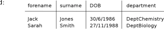
[image:23.595.191.463.583.634.2]

as named columns of a table. For example, theStud relation shown in Figure 2.1 has the attributesforename,surname,DOB(date of birth) anddepartment.

Figure 2.1: Relational table of students.

1

The consideration of semi-structured data as “self-describing” is somewhat misleading as it might be wrongly thought to suggest clear semantic description of such data. In particular, when considering the graph representation of semi-structured data, labels have only an informal meaning dependant on subjective interpretation of language, e.g. the imprecise term “location” could have many interpretations – address, map coordinates, URI, anatomical, etc.

(24)

The relational approach is essentially based on set theory, as well as on logic. For example, the

Studrelation (above) can be represented as set of studenttuples(rows or records),

Stud = { st1, st2, ... }

or, better, as

Stud = { student:st1, student:st2, ... }

where each student tuple is represented as a set of labelled atomic values, with labels being

attribute names, andattribute valuesas atomic values (strings of symbols between quotation marks to distinguish them from set names and attribute names),

st1 = { forename:"Jack", surname:"Jones",

DOB:"30/6/1986", department:"DeptChemistry" }

st2 = { forename:"Sarah", surname:"Smith",

DOB:"27/11/1988", department:"DeptBiology" }.

Let us consider the relational databaseUnivas the following set of (labelled) relations,

Univ = { departments:Dept, students:Stud, lecturers:Lect,

modules:Mod, courses:Course, ... }.

The relationsDept,Lect,ModandCoursewill not be further described, they are plausible example relations, likeStud, that could belong to a University database. Here the labels (or attributes) departments, students, lecturers, etc., give an informal description of what the sets Dept, Stud, Lect, etc., are about. These sets could be denoted differently, say as D, S,L, etc. Thus, strictly speaking the denotation of sets does not necessarily carry informational content. Hence the important role of labels (attributes e.g. forename) and atomic values (e.g. "Jack"), which are the proper carriers of basic information.

2.1.2 Relaxation of structural restrictions on relational data

Relational data with the given schemaR(A1, A2, ..., An)has a rigid structure with mandatory

attributesAifor associated tuple components. It is also known of the more general approaches

tonestedrelational databases [52, 54, 71] where attribute values could be relations. Say, in the above example we could reconsiderDeptChemistryas a set (instead of an atomic value) by omitting the quotation marks aroundDeptChemistryand adding the corresponding set equation further detailing the chemistry department:

DeptChemistry = { name:"Department_of_Chemistry",

lecturers:ChemLect,

modules:ChemMod,

(25)

Moreover, we could relax the requirement on students tuples to have a value for each attribute

forename,surname,ageanddepartment. For example, the DOB of a student could be absent by some reason, but some other information could be present, such as

email:"[email protected]"

or,

sex:"male".

Thus, relaxation of traditional structural restrictions on relational databases leads naturally to semi-structured databases, in fact, to the set theoretic approach where such data are considered asarbitraryset of (labelled) sets of sets, etc., to any depth, represented by set equations like above.

2.1.3 Semi-structured data

For simplicity, we consider semi-structured data as systems offlat set equations where a set equation consists of set namesiequated to a bracket expressionBi(¯s)like those considered in

the above example. In vector form this can be summarised as

¯

s= ¯B(¯s).

Flat bracket expression{l1:si1, . . . , ln:sin}is thought of as a set of labelled elements. In the

flat (non-nested form) only set namessi from the list of all set namess¯=s1, s2, ..., sn, may

participate as elements. Labelslj can be considered as analogous to attributes in the relational

approach, however, element labelling is optional with the default label being the empty label2 (ornull) which can be considered as invisible, such as the absence of labelling in theStud

set above. Formally our general approach does not consider atomic values such as"Jack",

"Jones", etc., from the example above. However, any atomic value can be simulated as a set consisting of one labelled empty set [41, 57, 61], such as

"Jack" = {’Jack’:{}}.

Strictly speaking, we should use single quotation marks for labels (often omitted for simplicity) and double quotation marks for atomic values. Of course, we can still use the denotation for atomic data like"Jack", but it should be understood as above.

2.1.4 Syntactical and conceptual set nesting

In the case where nesting is allowed (like the participation of {}in the above definition of atomic values, and also in more complicated cases) any set name si can be substituted with

(26)

equation could be rewritten with the nested right-hand side (and adding thestudentattribute) as follows,

Stud = {

student:{ forename:"Jack", surname:"Jones",

DOB:"30/6/1986", department:"DeptChemistry" },

student:{ forename:"Sarah", surname:"Smith",

DOB:"27/11/1988", department:"DeptBiology" }

}.

Here the nesting of data inside theStudset equation proves useful in avoiding the introduction of new set names, and thus eliminatingst1 andst2. Moveover, this demonstrates that set names in set equations play an auxiliary role, and can even be readily renamed in an analogous way to renaming variables in any ordinary algebraic equations. Thus the real information of such semi-structured data is carried by labels and set/element nesting. More generally, we could allow (and, in fact, will consider later) arbitrary nesting in the right-hand sides of set equations s¯ = ¯B(¯s). This can be evidently “unnested” or “flattened” by introducing new (fresh) set names and appropriate set equations. So, our restriction for non-nested systems of set equations (i.e. with non-nested right-hand sides) is not essential, but can simplify some considerations.

In fact, the notion of non-nested or flat system of set equations is only syntactical and, conceptually, flat systems of set equations allow arbitrary nesting with the participation of set names (corresponding to set equation) as elements

2.2 Hyperset theoretic view of semi-structured data

In the above approach to semi-structured data via systems of set equationss¯= ¯B(¯s)there was, in fact, no restriction on the form of these equations. Thus allowing not only arbitrarily nested, but also cycling data like in the simplest example of a set consisting of itself

Ω ={Ω}.

(27)

a situation that after several such “clicks” we will arrive back to the original table we started “clicking” with – like in the World-Wide Web by successive “clicking” we can possibly return to the Web page we started with. Moreover, from the informational or database point of view this can be quite meaningful.

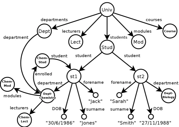
For example, let us consider the University database where formally the student setst1has the chemistry department setDeptChemistryas the member, and (possibly many) students are members of theChemStudset of enrolled chemistry students, as described by mutually recursive set definitions,

st1 = { forename:"Jack", surname:"Jones",

DOB:"30/6/1986", department:DeptChemistry }

DeptChemistry = { ..., enrolled:ChemStud, ... }

ChemStud = { student:st1, ... }

withChemStuda subset of the setStudof all university students. Any set (name)sican be

defined by referring to other set (names) as elements, etc., so that eventually we could possibly come to the original setsi – thus, arbitrary cycling is allowed.

There is more to say about the hyperset approach to semi-structured data on the conceptual level, in particular, on the concept of equality between sets (possibly denoted by different set names) but we will postpone this discussion to Section 2.4.1. On the current very preliminary level of consideration sets are thought simply as syntactical bracket expressions, or as represented by formal systems of set equations. In fact, we need an abstract concept of hypersets amongst which we could find a (unique) solution to any given system of set equations.

2.3 Graph or Web-like view

2.3.1 Graph representation of systems of set equations

Representation of semi-structured databases by systems of set equations presents a clear and mathematically well-understood2conceptual view of semi-structured data as (hyper)sets. But it also makes sense to consider visualisation of systems of set equations by the equivalent representation as (finite) labelled directed graphs. In fact, it is important for all considerations of this work that any given system of set equations can be considered as a labelled directed graph.

2

(28)

[image:28.595.103.410.110.328.2]

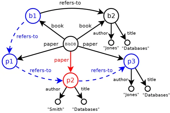
Figure 2.2: Semi-structured databaseUnivrepresented as directed graph.

In fact, most approaches to semi-structured databases typically consider them as labelled directed graphs, that is, semi-structured data is modelled as (finite) directed graphG=hN, Ei with L-labelled edges, where L is an infinite set of possible labels (l1, l2, . . ., etc., and the

empty label2),N is a finite set of nodes (s1, s2, . . ., etc.), andE is a finite set of edges with

each edgesi lk

→ sj being formally an ordered triple of the formhsi, sj, lki. For example, the

University database considered in Section 2.1 has the corresponding representation by directed graph shown in Figure 2.2.

The membership of labelled elementlabel:s2 to the sets1 (label:s2 ∈ s1) corresponds

to the labelled edge s1

label

−→ s2 (and vice versa), where set names si serve as (the unique

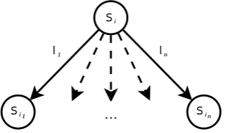
names of) graph nodes. In general, each set equation si = {l1 :si1, . . . , ln :sin} from the

system generates a fork of labelled edges si l1

−→ si1, . . . , si

ln

−→ sin outgoing from si, as

depicted in Figure 2.3. All those forks generated from every set equation give the corresponding representation as graph. Vice versa, any graph with labelled edges is evidently visualising a system of set equations, with one equation for each node so that each node is thought as a (hyper)set. Thus, graphs and (formal) systems of set equations are essentially equivalent concepts.

2.3.2 Graphs or systems of set equations as Web-like databases

(29)

[image:29.595.238.402.114.211.2]

Figure 2.3: Forking of labelled edges generated by the set equationsi ={l1:si1, . . . , ln:sin}.

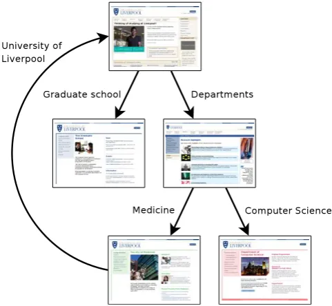
with markup tags denoting visualisation and hyperlink information. The following fragment of HTML code is an example of a hyperlink,

<a href="http://www.liv.ac.uk/">University of Liverpool</a>

what in our symbolism of labelled elements can be represented as

University of Liverpool : http://www.liv.ac.uk/

and visually (in Web browser) this hyperlink would appear as “clickable” fragment of text

University of Liverpool

with the URL hidden. Hiding of URLs corresponds to the idea mentioned above that set names (names of graph nodes) actually do not matter from the point of view of the proper information. Only labels on edges or the “clickable” links (and other text and visual content) on Web pages carry information, plus, of course, the graphical structure. That is, URLs play a different role than proper information in the WWW. In Figure 2.4 we consider browsing between hyperlinked HTML documents by “clicking” on such links. It is evident from this example that hyperlinked HTML documents can express arbitrary relationships, for example the cycle when browsing by “clicking” on the links,Departments,Medicine,University of Liverpool, and so on.

Thus, any hyperlink can be denoted by the labelled edge urli label

−→ urlj, suggesting the

(30)

[image:30.595.155.396.201.423.2]

governed by some organisation or company, and possibly not allowed to be arbitrarily extended by anybody in the world (like typical databases). Additionally, WDB (or semi-structured data) can also have a schema restricting the shape of the WDB, but not necessarily so rigid like in the case of relational databases, see for example [9, 41, 57]. However, we will not go further into these details.

Figure 2.4: Browsing of hyperlinked HTML documents on the University of Liverpool website.

2.3.3 Distributed WDB

Any WDB represented as a system of set equationss¯= ¯B(¯s)can be quite big, and naturally divided into subsystems of set equations. Each subsystem corresponds to a XML-WDB file (see Chapter 10 for details of the XML-WDB representation) containing only some of the equations (desirably closely interrelated by a subject matter). Moreover, these files could be distributed between various servers over the world, like HTML files on the World-Wide Web. It may happen that set equations defined in some WDB file may involve set names defined by equations in other (non-local) WDB files.

Furthermore, when considering the real application of WDB distribution proves useful in the creation and management of (potentally large) databases, such as the plausible distribution of the University WDB. Let us consider that in the case of the University WDB, set equations might be distributed between many WDB files, let us say by department. Therefore, the WDB filehttp://www.liv.ac.uk/ChemistryDepartment.xmlcould contain the following subsystem of set equations3:

3

(31)

DeptChemistry = { ..., enrolled:ChemStud, ... }

ChemStud = { student:st1, ... }

Likewise, the WDB filehttp://www.liv.ac.uk/BiologyDepartment.xmlcould contain the subsystem of set equations:

DeptBiology = { ..., enrolled:BiolStud, ... }

BiolStud = { student:st2, ... }

Moreover, there could also be the WDB file Students.xml containing the set equations

st1 = {...} and st2 = {...}. Thus, the set names st1, st2, etc. participating,

respectively, inChemistryDepartment.xmlandBiologyDepartment.xmlwould now be described as sets in another file. In this case, we should consider the full versions of the simple set names,st1, st2, etc., described inhttp://www.liv.ac.uk/Students. xml, as discussed below.

2.3.3.1 Full versus simple set names

Taking into account the above example, any given set name should be considered as afull set name, consisting of WDB file URL andsimple set name(with the simple set name described within the WDB file). For example, in the distributed University WDB considered above, the full set name of the biology studentst2would be

http://www.liv.ac.uk/Students.xml#st2

with the WDB file URL and simple set name delimited by# symbol. However, in practice it suffices to use simple set names in the left-hand side of set equations, and also for those occurrences of set names appearing in the right-hand side of set equation definitions if they are defined in the same WDB file. In particular, the author of a WDB file can freely use any simple set name (as such or as part of full set names) without the danger of clashes with simple names participating in the other WDB files.

However, there is one subtle point: if a simple set nameset_nameoccurs twice in some WDB file, once as a simple set name and again as part of a full set name url#set_name

(withurl referring to some different WDB file). Then in the latter case it refers to another file where the corresponding equation is defined, even if the current file already contains the equationset_name = {...}. Thus, these two occurrences are actually different set names because their corresponding full set names are indeed different. Of course, each set name must be defined either in the same or some other WDB file. Otherwise it is considered as syntactical error. Thus, it is necessary to download some WDB files whose URLs appear in full set names of the given file to confirm the existence of defining equations of the referenced set names.

(32)

2.4 Hyperset data considered abstractly

The notion of WDB as a system of set equations presents a low level, syntactical understanding of semi-structured data. However, conceptually (and semantically) WDB is understood as consisting ofabstract hypersets (like relational database consists of abstract relations). The hyperset approach considers WDB as an arbitrary finite system of set equations, each set equation consisting of set name equated to corresponding bracket expression. But the intended meaning of such a syntactical expression is a set of labelled elements,notan ordered sequence. Therefore according to this (hyper)set theoretic approach ordering and repetition of elements in a bracket expression should be completely ignored. That is, ignoring ordering and repetitions has some bothoperationalandconceptualconsequences.

This can possibly lead to equality between different set names si and sj denoted as

si = sj and meaning thatsi andsj denote the same abstract hyperset, or strictly denoted as

si ≈sj(to avoid possible misunderstanding ofsi =sjas the assertion that these set names are

identical, and to stress on the particularly important role of this concept of equality). In fact,≈ is the well known concept in the context of graphs calledbisimulation relationbetween graph nodes or, in our case, between set names [3, 5, 61]. As the role of this relation is crucial for the hyperset approach to semi-structured databases, this approach is therefore more than pure graph theoretic, as considered in the approaches to semi-structured databases as graphs e.g. in [1, 2, 11, 18, 19, 36, 46] or as XML tree-like data e.g. in [23, 33]. Note that, however, [11] is also heavily based on the bisimulation relation, it is rather a graph than a hyperset approach as was argued in [61].

2.4.1 Bisimulation – preliminary considerations

In general, the bisimulation relation between set names (graph nodes) of a WDB, i.e. a system of set equations, and the corresponding recursive algorithm is based on the idea that any two sets are equal if for each (labelled) element of the first set there exists an equal (bisimilar) element in the second set (and vice versa). Bisimilar set names are said to denote the same abstract (hyper)set. The bisimulation relation will be further described in Chapter 4, with formal theoretical definition, and practical considerations for its implementation. We consider that this hyperset approach to WDB is worth implementing as it suggests a clear and mathematically well-understood view on querying such semi-structured data.

(33)

especially in the case of distributed WDB. Therefore, we devote Part II to some approach of dealing with this problem practically.

2.4.1.1 Example

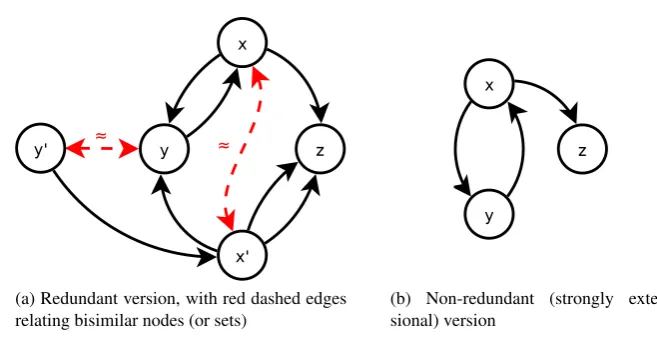
Consider the set equations below, where triviallyx≈x0holds because our (hyper)set approach ignores the ordering and repetition of elements:

x={y, z}

x0={z, y, z}.

However, set names (or graph nodes) may be equal (bisimilar) for some “deeper” reason than forxandx0above. Let us consider the above example extended with the (recursive) definitions of the setsz,yandy0:

z={}

y={x}

y0 ={x0}.

The sets y and y0 both contain one element of syntactically differing set names (x and x0

respectively), thus suggesting that y andy0 might not be equal. However, the bisimulation relation defines two sets as equal if for each element of the first set there exists an equal (or bisimilar) element in the second set, and vice versa. In the case above we already know that

x≈x0holds, and according to this informal definition of bisimulation all of the elements ofy

are bisimilar to the elements ofy0, and vice versa. Therefore we can deduce that, in fact,y ≈y0

holds.

Let us now consider the strongly extensional version of this system of set equations obtained by eliminating the redundant set names x0 andy0, and omitting repetitions. Thus, after “collapsing” the bisimilar nodesx0 toxandy0toy, and omitting element repetitions, the resulting system of set equations is

x={y, z}

y ={x}

z={}.

(34)

(a) Redundant version, with red dashed edges relating bisimilar nodes (or sets)

[image:34.595.104.433.115.284.2]

(b) Non-redundant (strongly exten-sional) version

Figure 2.5: Graphical representation of a trivial WDB (cf. corresponding set equations above).

2.4.2 Redundancies in WDB

The above example, although artificial, demonstrates that bisimilarity between set names introduces redundancies into WDB. However, the crucial question in implementing the hyperset approach to WDB is whether the bisimulation relation (≈) can be computed in any reasonable and practical way. Some possible approaches and views are outlined below.

In principle, the occurrence of bisimilar nodes in a realistic WDB (i.e. redundancies) should be infrequent. Therefore, such rare redundancies can be eliminated by supporting WDB in astrongly extensionalstate, with redundancies detected or even eliminated instantly as soon as they might potentially appear. Trivially, after eliminating redundancies equality between sets (i.e. bisimulation relation between set names or graph nodes) becomes the identity relation. However, eliminating redundancies is more expensive than only detecting them i.e. just computing bisimulation relation on the WDB. Thus, supporting WDB in strongly extensional form may be reasonable option when WDB is not large.

WDB should not be assumed to be just another version of WWW, freely extensible by anybody in the world. That is, an appropriate discipline of working with WDB could make the problem of bisimulation practically resolvable. Let us now consider several ways by which redundancies can appear.

2.4.2.1 Redundancies arising during query execution

(35)

WDB do not refer to new ones in WDB0, thus WDB remains self-contained. Therefore, the new bisimulation relation (≈0) on WDB0 restricted to those set names in WDB coincides with the identity relation on WDB. Moreover, the algorithm of query execution could be amended in such a way that as soon as new (auxiliary) set names are generated (likeresin Section 3.3) any possible redundancies will be eliminated immediately. It should also be taken into account that the extensions WDB0 arising during query execution have several specific types, and are sufficiently simple and small, thus making the process of detecting/eliminating redundancies easier, see also [40, 42], but we will not go into the details here.

2.4.2.2 Redundancies which can appear during a local update

Local updates of WDB files are more problematic because previously non-bisimilar nodes outside this file may become bisimilar due to possible links (or paths) to the local nodes with changed/added meaning. The appropriate (more efficient than the standard) strategy of detecting/removing all such redundancies is not so straightforward and needs to be developed yet. However, taking into account the locality of changes, this task does not seem to be unrealistic.

2.4.2.3 Deliberate redundancies

Deliberate redundancies in WDB can also appear with the same aim as mirroring in WWW. But, if there is a requirement to officially registered such mirroring in the WDB, then such deliberate redundancies should most plausibly be dealt with in a quite feasible way.

2.4.2.4 Local versus global bisimulation

Unlike the other considerations above, we will consider the “local/global” approach and its implementation for supporting bisimulation relation on WDB (in background time) in more detail (see Part II). Now we present only some general introductory comments on this idea.

Assume that all WDB nodes are divided into classes Li according to their sites (WDB

servers) or even files. There is a quite natural definition of local (i.e. computed locally) lower and upper approximations (≈L

−,≈L+) to the global bisimulation relation (≈) on the whole WDB:

n1≈L−n2 ⇒n1 ≈n2 ⇒n1 ≈L+n2

These approximations can help to compute and to permanently support global bisimulation in a distributed way in background time. Moreover, we could require local independence

(≈L

(36)

2.4.3 Bisimulation invariance

The hyperset approach assumes considering WDB (graphs or systems of set equations) up to bisimulation. Therefore, it is an important requirement for set theoretic operations and relations to be bisimulation invariant, that is to preserve the bisimulation relation. Although not fully proven here, it can be shown [58] that all definable queriesqof the hyperset∆-query language4 (see Chapter 3) are bisimulation invariant:

¯

x≈y¯=⇒q(¯x)≈q(¯y) (for set valued queries) ¯

x≈y¯=⇒q(¯x)⇔q(¯y) (for boolean queries).

For example, in the case of the set theoretic operation union we have:

x1 ≈y1 &x2 ≈y2 ⇒(x1∪x2)≈(y1∪y2).

This actually means that we work with (abstract) hypersets rather than just with graph nodes or set names, however the operational semantics of the language∆is based on the syntactical manipulations of set equations [61]. The point is that the semantics of the language∆respects bisimulation and completely agrees with the hyperset theory [3, 5].

In particular, x1 ∪x2 is defined as a new set name, say u, with corresponding new set

equation u = {. . . , . . .}, where the first “. . .” is the content of the right-hand side of the equationx1 ={. . .}from the given WDB, and similarly for the second “. . .” and the equation

x2 ={. . .}. The uniony1∪y2 is computed in the same way from set equations fory1 andy2

giving rise to new set name,u0, and the corresponding set equationu0 ={. . . , . . .}. Then the conclusion of the above bisimulation invariance condition for ∪actually meansu ≈ u0, and can evidentially be shown.

Note that the membership relationx∈ yfor two sets (considering the unlabelled case for simplicity) is defined to be true if the set equation for y involves some set name x0, where

y = {. . . , x0, . . .}and, moreover,x ≈x0. Additionally, it can be shown that the membership relation is also bisimulation invariant:

x1≈y1&x2 ≈y2 =⇒ x1∈x2 ⇐⇒ y1∈y2

For all other constructs of the∆-language the operational semantics maybe more complicated, however, it follows that they also agree with this intuitive (abstract) set theoretical meaning. The syntax and semantics of the ∆-query language will be further detailed in Sections 3.1 and 3.2, with some further indications of the operational semantics in terms of set equations

4

(37)

detailed in Section 3.3.

2.4.4 Anti-Foundation Axiom

Finally, we do not go into full mathematical details on hypersets, however, we could assert the following form ofAnti-Foundation Axiom(AFA) [3, 5], which holds in the universe of abstract (in our case finite) hypersets:

Any system of set equationss¯= ¯B(¯s)has a unique abstract hyperset solution for set namess¯making these equations true.

Therefore, set names of any WDB (as system of set equations) denote quite concrete, uniquely defined abstract hypersets. In this sense each set name (in a∆-query) serves as a set constant (relative to the given WDB) denoting a unique hyperset. Note that, the∆-language also has set variables which can be quantified unlike constants.

(38)

(39)

Query language

∆

3.1 The syntax

There has already been much theoretical considerations on (some versions of) the∆(Delta) query language to hyperset/WDB databases [40, 41, 43, 57, 61]. The two main syntactical categories of∆are:

• ∆-termsrepresenting set valued operations over hypersets (set queries), and

• ∆-formulasrepresenting truth valued operations (boolean queries).

Note that the denotation ∆bears partly from the well-known class∆0 of bounded formulas

introduced by Levy, although ∆, as defined here, denotes a wider language. It is based on the basicorrudimentaryset theoretic languages of Gandy [30] and Jensen [39]. Moreover, inclusion of set theoretic operators: transitive closure (TC), recursion (Rec) and, for the case of hypersets, decoration (Dec) (the latter due to Forti and Honsell [29] and Aczel [3]), allows to define in∆exactly all polynomial time computable operations over hypersets represented as WDB, thus demonstrating and characterising theoretically its rich expressive power (assuming that a linear order on labels is given) [43, 56, 57, 58]. The operators of∆are defined as follows:

h∆-termi::=hset variable or constanti ∅ {l1 :a1, . . . , ln, an}

[

a TC(a)

{l:t(x, l)|l:x∈a&ϕ(x, l)} Recp.{l:x∈a|ϕ(x, l, p)} Dec(a, b) h∆-formulai::=a=b l1 =l2 l1 < l2 l1 R l2 l:a∈b ϕ&ψ ϕ∨ψ ¬ϕ

∀l:x∈a.ϕ(x, l) ∃l:x∈a.ϕ(x, l)

The intuitive set theoretic semantics of the majority of the above constructs should be well-understood by anyone with the minimal mathematical background in set theory and logic. In the above constructs we denote:a, b, . . .as (set valued)∆-terms;x, y, z, . . .as set variables;

(40)

l, lias label values or variables (depending on the context);l :t(x, l)is anyl-labelled∆-term

tpossibly involving the label variable l and the set variablex; andϕ, ψ as (boolean valued) ∆-formulas. Note that labels li participating in the∆-term {l1 :a1, . . . , ln : an} need not

be unique, that is, multiple occurrences of labels are allowed. This means that we consider arbitrary sets of labelled elements rather than records or tuples of a relational table where li

serve as names of fields (columns).

The binding label and set variablesl, x, pof quantifiers, collect, and recursion constructs should not appear free in the bounding terma(denoting a finite set). Otherwise, these operators may become unbounded and thus, in general, non-computable. For example, let us consider the universal quantifier ∀l :x ∈ {. . . , l :x, . . .}.ϕ(x, l) which becomes unbounded due to the quantified variables l:x participating in the bounding term {. . . , l:x, . . .}. In fact, as

l:x ∈ {. . . , l:x, . . .}is always true the above quantified formula proves to be equivalent to unbounded one:∀l:x.ϕ(x, l).

3.2 Intuitive denotational semantics

Any∆-query without free variables has either: i) (hyper)set value in the case of∆-terms, or ii) boolean value in the case of∆-formulas. Those participating set variables or set constants represent abstract hypersets (and thus correspond to set names in WDB), whereas participating label variables or label constants represent label values (corresponding to strings of symbols).

The intuitive meaning of∆-queries is described by thedenotational semantics, that is what any expression denotes1. For the purposes of implementation ∆-queries are also described by means of their operational or computational semantics (see Section 3.3) which must be coherent with our intuitive denotational semantics. Here we will also rely on intuition, without presenting any precise argument. In fact, the required coherence will be pretty much evident. So, we can concentrate on examples of queries and implementation aspects.

3.2.1 Boolean valued expressions —∆-formulas

Equality(=) and thealphabetic ordering(<) between labels is understood standardly. In the theoretical∆-language the relationRover labels is any easily computable relation over labels, however, in the implemented∆-language described in this thesis we considerRas any of the followingsubstringrelations

1_{There is a deep mathematical theory of denotational semantics of programming languages based on Domain}

(41)

∗l1=l2 l1∗=l2 ∗l1∗=l2

where the wildcard∗represents any string of symbols. In principle we could include into the language more relations over labels, but in the implementation there are only<and substring relations, and the user currently has no way to define more primitive relations over labels. It should be noted that equality between ∆-terms, a = b or, for technical reasons, a ≈ b, is understood as the equality of abstract hypersets denoted by these terms and, as such, is computed by the bisimulation algorithm discussed in Chapter 4. That is, when we discuss hypersets abstractly, we use =. But when considering bisimulation algorithm to determine whether two set names or graph nodes denote the same abstract hyperset, we use ≈. In the implemented version of the language we have only =which, of course, involves calling the bisimulation algorithm, but this is hidden from the user who, therefore can think on hypersets abstractly. Moreover, bisimulation is implicitly involved in the (computational) meaning of the

membershiprelation according to the equivalence

l:a∈b ⇐⇒ ∃m:x∈b.(m=l&x≈a)

informally having the meaning: find an outgoingl-labelled edge frombwhich leads to some nodex bisimilar to a. But, thinking abstractly, l:a ∈ bsays simply that a is anl-labelled element ofb.

Thelogical operators(&,∨,¬) have the usual meaning from propositional logic and can be used to form logical sentences from∆-formulas. Universal quantificationcan be understood in terms of conjunction:

∀l:x∈a.ϕ(x, l) ⇐⇒ ^

li:xi∈a

ϕ(xi, li)

andexistential quantificationin terms of disjunction:

∃l:x∈a.ϕ(x, l) ⇐⇒ _

li:xi∈a

ϕ(xi, li)

assuming thata={l1 :x1, . . . , ln :xn}. It is evident from this definition that quantification

(42)

Note that when a quantified formula participates as a subformula of a bigger formula or of a term the technical problem arises where exactly this (sub)formula is finished, that is what is the scope of the quantifier. In the implemented∆-language (Appendix A.1) there is a discipline of using parentheses to find unambiguously the scope of quantifiers, both intuitively and by the implemented parser (and contextual analysis algorithm). Say, in

∀l:x∈a .(ϕ&ψ&χ)

the scope of the quantifier is the whole expression in the parentheses. But the general informal rule is: the scope of any quantifier is as small as possible. For example, in

(∀l:x∈a . ϕ&ψ&χ)

the multiple conjunctions requires some compulsory external parentheses (exactly as shown), and then the scope of the quantifier is either ϕ (excludingψ andχ) or some initial part of

ϕ, if syntactically meaningful at all. We will not give the formal definition which is usually widely known and intuitively evident. For the precise definition of the scope of quantifiers, declarations, etc. the reader should, first, inspect the relevant part of the ∆-language syntax in Appendix A.1 and, most importantly, read the Section 9.2 on contextual analysis which, in fact, served as a rigorous conceptual guidance for us to implement the language correctly.

3.2.2 Set valued expressions —∆-terms

The set constantempty set (∅) denotes the set{} having no elements. In general, set values are represented symbolically by either: set constants, set variables or ∆-terms. Furthermore, “literal” set values can be introduced with the enumeration expression {l1 :a1, ..., ln: an}

which can create new sets, possibly with nesting if someaiare also enumeration expressions,

however,aimay also be arbitrary∆-terms.

The collection operation{l:t(x, l) | l :x ∈ a & ϕ(x, l)} denotes the set of labelled elementsl:t(x, l)witht(x, l)a∆-term depending on the set and label variableslandx, where

l:xranges over the set a, for which the ∆-formula ϕ(x, l)holds. We can also consider the more special case of collection called the separation operation{l:x ∈ a | ϕ(x, l)} which denotes the set of labelled elementsl:xinafor whichϕ(x, l)holds.

The (unary)union operationS

ais understood as the (multiple) ordinary union over the elements ofa. Let us assumea={l1:a1, . . . , ln:an}then

[

(43)

with the ordinary union used in the right-hand side of equality. In particular, this also shows that the ordinary union is definable by means of the unary union and enumeration operators. This is only the simplest example of expressibility in∆. As we mentioned, this language has, in fact, very high expressive power exactly corresponding to polynomial time computability over hereditarily-finite hypersets2.

The transitive closure TC(a) denotes the set of (labelled) elements of elements, . . . , of elements ofaincludingaitself. This can also be written (not fully formally, say, due to . . .

present) as:

l:x∈TC(a) ⇐⇒l:x∈x0 ∈. . .∈xn=a∨

(l=2&x=a)

withxisome intermediate elements in the membership chain, each belonging to the nextxi+1

with some labelliwhose value is not important. In particular, we let2:a∈TC(a).

The above core constructs of the∆-language extended with the two additional constructs recursion and decoration (introduced below) define all polynomial time computable operations and relations over hypersets (represented as WDB); see the precise formulations in [41, 43, 57].

3.2.2.1 Recursion operation

The recursionoperatorRec p.{l:x ∈ a | ϕ(x, l, p)}defines a subset π of the set denoted by (the ∆-term) a, obtained as the result of stabilising (due to finiteness ofa) the inflating sequence of subsets ofadefined iteratively as:

p0 =∅

p1 =p0∪ {l:x∈a|ϕ(x, l, p0)}

p2 =p1∪ {l:x∈a|ϕ(x, l, p1)}

. . .

pk+1 =pk∪ {l:x∈a|ϕ(x, l, pk)}.

Evidently, all∅ =p0 ⊆ p1 ⊆. . .are subsets ofa. Asais finite, pk = pk+1 =pk+2, . . . for

somek, and this stabilised value, denoted above asπ, is taken as the value of the recursion operator.

2

(44)

3.2.2.2 Decoration operation

Recall that in Chapter 2 graph nodes were shown to denote (hyper)sets, and vice versa, arbitrary hereditarily-finite hyperset can be represented in this way.

Now, we shall consider finite graphs in set theoretic terms. Traditionally, this is done by defining a graph as a set of ordered pairs where ordered pairs represent graph edges, for example ha, bi denoting the edge a → b. Here (the arbitrary sets) aandb, play the role of the source and target vertices of the edge a → b. Thus, any set g of ordered pairs can be treated as a graph. Formally such ordered pairs are represented as the sets containing two elements labelled byf st andsnd respectively, such as{f st:a, snd:b}. That is, we define ha, bi={f st:a, snd:b}. Any labelled ordered pairl :{f st:a, snd:b}represents a labelled edgea→l b. In general, we can consider absolutely arbitrary hypersetgas representing a graph. Indeed, we can take into account only those elements ofgwhich happen to be ordered pairs, and ignore the other non-pair elements. This will make the operation of decoration defined below applicable to the arbitrary hypersetgwhat is convenient. Otherwise the formulation of the language∆would be more complicated. Also, the arbitrary setvmay either participate as an element of the ordered pairs ofg, i.e. serving as ag-vertex, or, otherwise, it is considered as an isolated vertex of the graphg. In this sense each setvserves as ag-vertex.

Definition 1. The abstract set theoreticdecoration operatorDec(g, v) =dtakes two arbitrary input setsgandvwhere the former represents a graph as a set of ordered pairs, and the latter represents some vertex v of this graph. It outputs a new (hyper)set d corresponding to the

v-rooted graphgaccording to the first paragraph of this section.

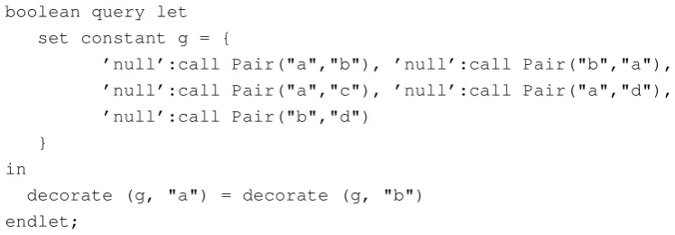
Note that decoration is the only operator in∆which allows for the construction of cyclic hypersets, like Ω = {Ω}, from the ordinary “uncycled” sets (of sets of sets,. . . ) of finite depth. For example, consider thetrivial cyclicgraphgdefined by the following system of set equations,

g={ {f st:a, snd:a} }

a={}

The result of applying decoration to the graphgand the participating vertexawould be,

Ω ={Ω}

(45)

from Section 2.4.4 guarantees thatΩis a unique hyperset denoted byDec(g, a)(and the same for arbitraryganda).

This operator can also be reasonably called the plan performance operator [61] because its input(s) can be considered as a graphical plan for the construction of a hyperset with the output being the resulting abstract hyperset. Imagine that we have a plan of a Web site (i.e. of a system of hyperlinked Web pages) and thatDecis a tool (or query) which automatically creates all the required Web pages. See also Section 3.5.3 for a more involved example of using the decoration operation for defining a restructuring query.

3.3 Operational semantics

Consider any set or boolean queryq which involves no free variables and whose participating set names (constants) are taken from the given WDB system of set equations. Resolving q

consists in the following two macro steps:

• Extendingthis system by new equationres=qwithresa fresh (i.e. unused in WDB) set or boolean name, and

• Simplifyingthe extended system:

WDB0=WDB+ (res=q)

until it will contain only flat bracket expressions as the right-hand sides of the equations or the truth valuestrueorfalse(if the left-hand side is boolean name).

After simplification is complete, these set equations will contain no complex set or boolean queries (likeqabove). In fact, the resulting version WDBresof WDB will consist (alongside

the old equations of the original WDB) of new set equations (new set names equated to flat bracket expressions) and boolean equations (boolean names equated to boolean values,trueor

false). This process of computation by extensionandsimplificationwas described in [61] as reduction steps

W DB0W DB1. . .W DBres

whereW DB0 is the initial state ofW DBextended by the equationres=q, andW DBresis

(46)

∆ expressions into simpler, semantically equivalent, equations. Note that the rewrite rules described here are based on those in [61] but extended to the labelled case as considered in this thesis. In general, rewrite steps are denoted by the symbol which means “transforms to”. Firstly, let us assume participation of the set names s, p, r in the rewrite rules below, which correspond to the set equations

s={l1:s1, ..., la:sa},

p={m1:p1, ..., mb:pb},

. . .

r ={n1:r1, ..., nc:rc}

existing either in the initial W DB or in the current reduction W DBi. The operational

semantics for the∆operators (except for recursion, decoration, transitive closure, bisimulation and label relation operators) are described as the reduction rules

res=t(t1, . . . , ta)

              

res =t(res1, . . . , resa),

res1 =t1,

. . . resa =ta.

res={l:s, m:p, . . . , n:r}– no further reduction required onces, p . . . , r,are set names, res=s∪p∪. . .∪rres={l1:s1, ..., la:sa, m1:p1, ..., mb:pb, . . . , n1:r1, ..., nc:rc},

res=[sres=s1∪. . .∪sa,

res=TC(p)– operational semantics described in Section 8.1.5, res={l:x∈p|ϕ(l, x)}res={mi1:pi1, . . . , mib0:pib0}

wheremij:pij are all thosemi:pi∈pfor whichresi =ϕ(mi, pi)resi =true,

res={t(l, x)|l:x∈p&ϕ(l, x)}res={t(mi1:pi1), . . . , t(mib0:pib0)}

wheremij:pij are all thosemi:pi∈pfor whichresi =ϕ(mi, pi)resi =true,

res=Recp.{l:x∈a|ϕ(l, x, p)}– operational semantics described in Section 8.1.3, res=Dec(a, b)– operational semantics described in Section 8.1.4,

res=∀l:x∈p . ϕ(l, x)res=ϕ(m1, p1) &...&ϕ(mn, pn),

res=∃l:x∈p . ϕ(l, x)res=ϕ(m1, p1)∨...∨ϕ(mn, pn),

(47)

res=false&ϕres=false, res=ϕ&falseres=false, res=ϕ∨ψres=¬(¬ϕ&¬ψ), res=¬falseres=true,

res=¬trueres=false,

res=l:s∈pres=∃m:x∈p .(s=x&l=m),

res=x=yx≈y– operational semantics described in Section 4.2.1, res=l R m– operational semantics described in Section 3.2.1.

The implementation of∆-query execution is based on this process of reduction except for the ∆-terms: recursion, decoration, transitive closure described in Section 8.1.3, Section 8.1.4 and Section 8.1.5 respectively; and the∆-formulas: set equality (bisimulation) and label relation operators described in Section 4.2.1 and Section 3.2.1 respectively.

3.3.1 Examples of reduction

The above process of computation by reduction is quite natural as shown in the following examples.

3.3.1.1 Example elimination of complicated subterms

Let us consider the reduction of the queryq = S

q1 containing the complex subqueryq1. In

general, any complicated term t(t1, . . . , tn) can be simplified by invoking the splitting rule

which transforms the equationres=t(t1, . . . , tn)to the resultant equations

res=t(res1, . . . , resn)

res1=t1

. . . resn=tn

Therefore, the complicated queryres =S

q1 can be split into two subqueries,res =Sres1

(48)

3.3.1.2 Example reduction of union

In the case of our union query having the particular formq=S_{

l:s, m:p, n:r}wheres, p, r

represent set names, it follows that the equationres=qis reduced by the following steps:

1. Split the complicated equationres=S

{l:s, m:p, n:r}resulting in the equations:

res=[res1

res1={l:s, m:p, n:r}

wheres, p, rare set names, and hence do not require further splitting.

2. Reduce unary unionres=S

res1to multiple union resulting in the equation:

res=s∪p∪r

with the unary union reduced to multiple unions over the elements of the setres1 (the

set namess, p, r).

3. Reduce multiple union res = s ∪ p ∪ r to the bracket expression resulting in the equation:

res={l1:s1, ..., li:si, m1:p1, ..., mj:pj, n1:r1, ..., nk:rk}

assuming that the current extension of the original WDB already contains the simplified equationss={l1:s1, ..., li:si},p ={m1:p1, ..., mj:pj}andq ={n1:q1, ..., nk:rk}.

Here multiple union over the setss, p, ris reduced to the bracket expression containing the elements of these sets.

In general, most of the∆operators can be resolved using the above reduction rules except for recursion, decoration, transitive closure, bisimulation and label relation operators. In fact, there is no common framework for describing the operational semantics for all the∆operators, with the latter exceptions described as lower-level algorithms in Chapters 4 and 8.

The main conclusion is that after reduction we will have the equationres ={. . .}of the required form whose right-hand side should involve no complicated terms or formulas, only set names either from the original WDB or new set names introduced during reduction (likeres1

above) together with the corresponding equations of the required form. Thus, execution of a query extends the original WDB to WDBres(simplification of WDB0 above). This extension