Optimal Consumption under Deterministic Income
J. Eisenberg∗, P. Grandits†and S. Thonhauser‡ September 8, 2011
Abstract
We consider an individual or household endowed with an initial wealth, having an income and consuming goods and services. The wealth development rate is assumed to be a deterministic continuous function of time. The objective is to maximize the discounted consumption. Via the Hamilton–Jacobi–Bellman approach we prove the existence and the uniqueness of the solution to the considered problem in the viscosity sense. Furthermore we derive an algorithm for explicit calculation of the value function and optimal strategy. It turns out that the value function is in general not continuous. The method is illustrated by two examples.
Key words: optimal control, optimal consumption, value function, Hamilton–Jacobi– Bellman equation, viscosity solutions, semi-continuous envelopes.
2010 Mathematical Subject Classification: Primary 93B05 Secondary 49L20, 49L25
1
Introduction
Maximizing the expected utility of an individual from consumption and by controlling
investment has been a classical problem in mathematical finance for a long time. The
interested reader is referred to papers by Karatzas et al. [8, 9] or Cox and Huang [5].
In actuarial science consumption is often interpreted as dividend payout. Numerous papers
and books have been written on the topic of dividend maximization in the framework
of the classical risk model, its diffusion approximation or piecewise deterministic Markov
processes. A summarization of actuarial findings of the last 50 years can be found in Avanzi
[1] or Albrecher and Thonhauser [2].
In this paper we consider an individual or household whose income stream is described by a
deterministic process with continuous drift function. The drift function can attain negative
∗Department of Financial and Actuarial Mathematics, Vienna University of Technology. The research of
this author was supported by
†Department of Financial and Actuarial Mathematics, Vienna University of Technology. The research of
this author was partly supported by
values or be even periodic, whereas the assumption of a non-negative drift is common
in literature. A suitable example provide households with income depending on seasonal
agriculture or tourism, which is characteristic for developing countries.
We assume that the primal interest of the individual/household is to maximize the
cumu-lated value of discounted consumption from a given time up to a finite time horizon. Or,
in other words, to maximize cumulated discounted utility from consumption, given a linear
utility function. One may notice that in the literature the dividend maximization problem
is usually stated on an infinite time horizon. The present problem formulation can be
re-garded as a non stochastic limiting case of Grandits [7], who deals with a pure consumption
maximization problem on a finite time horizon for a diffusion type wealth process.
Upon first sight the problem seems to be relatively easy to solve. However, some
diffi-culties arise such as that the value function turns out to be discontinuous even in
semi-continuity sense. Furthermore for applying the viscosity solution approach to the associated
Hamilton–Jacobi–Bellman equation we also have to take into account the discontinuity of
the considered value function. For semi-continuous viscosity solutions the problem of
ex-istence and uniqueness of a solution to Hamilton–Jacobi–Bellman equations with convex
Hamiltonians was dealt with by Barron and Jensen [3]. There the main idea is to transfer
the uniqueness requirement on solutions to their lower semi-continuous envelopes. In this
paper we will first use the concept of weak comparison, described for example in Fleming
and Soner [6], and finally show the strong uniqueness using specific properties of the value
function. For a general introduction into the theory of viscosity solutions see for example
Bardi and Capuzzo-Dolcetta [4].
The contribution of the present paper, beyond the discussion of the HJB approach, is to
establish an algorithm that allows to determine a closed form expression for the value
func-tion and the optimal strategy.
The paper is structured as follows. At first we give a mathematical formulation of the model
and state some important properties of the value function. Section 2, which is the main
part of the paper, is dedicated to algorithm derivation. The Hamilton–Jacobi–Bellman
approach is discussed in Section 3. For the sake of clarity of presentation we postpone the
Let us now start with the model formulation. The deterministic wealth process minus
consumption is given by:
• dXC
t =µtdt− dCtwithX0− =x and for 0≤t≤T,
• µt is continuous on [0, T] with only finitely many zeros in [0, T],
• C = (Ct)t∈[0,T]is cumulated consumption, c`adl`ag, increasing, ∆Cs≤XsC−.
The value of a given strategy is given by
J(0, x, C) =
Z τ−
0−
e−βt dCt+e−βτXτC ,
whereβ >0 is some discounting rate andτ = inf{t >0|XC
t <0} ∧T. Of courseτ depends
onC, if some distinctions are needed we will indicate them.
For application/derivation of some dynamic programming principle we need
XsC =x+
Z s t
µrdr−Cs, for 0≤t≤s≤T andXt−=x ,
J(t, x, C) =
Z τ− t−
e−βsdCs+e−βτXτC .
We tacitly assume the adaptions on the definitions of τ and C. We write C(t, x) for the set of admissible consumption strategies when starting at timet at levelx≥0. The value function of the associated maximization problem is given by
V(t, x) = sup
C∈C(t,x)
J(t, x, C) for (t, x)∈[0, T)×[0,∞),
V(T, x) =e−βTx forx∈[0,∞), (1)
V(t, x) = 0 for (t, x)∈[0, T]×(−∞,0).
In the following we will denote the requirements V(t, x) = 0 for (t, x) ∈ [0, T]×(−∞,0) andV(T, x) =e−βTx forx∈[0,∞) by (P1).
For later purpose we mention that for s ≥ τ we have Cs =Cτ− and Xs = Xτ, i.e.
con-sumption stops at the event of ruin.
The reader may notice that we assume a strategy to be c`adl`ag and hence the controlled
process XC as a post-consumption process, compare Schmidli [11, p. 80]. As a
large consumption leading to ruin in the value function. In the following Lemma we state
useful properties of the value function, which can be obtained immediately from the model
assumptions.
Lemma 1.1
The value functionV(t, x)fulfils
• V(t, x) is increasing inx, (P2)
• V(t, x)≤e−βtx+λ(t) forλ(t) =RT t |µs|e−
βsds. (P3)
Proof: Lety > x and C be anε-optimal strategy at (t, x), i.e. V(t, x) ≤VC(t, x) +ε. For
initial capitaly attconstruct a strategy ˜Cas follows: payouty−ximmediately and follow the strategyC. Thus, we have
V(t, y)−V(t, x)≥VC˜(t, y)−VC(t, x)−ε= (y−x)e−βt−ε .
Becauseεwas arbitrary, we obtain the result.
For every admissible consumption strategyC it holds
Z τ− t−
e−βsdCs+e−βτXτC ≤xe−βt+ Z τ
t
e−βs|µs|ds .
It followsV(t, x)≤e−βtx+RT t |µs|e−
βsds.
2
Optimal Strategy - Construction of a Solution
The following Lemma turns out to be crucial for the construction of the optimal
consump-tion strategy.
Lemma 2.1
Assume that in (t, x) ∈ [0, T]×[0,∞) it is optimal to payout ∆Ct. Then for (t, y) with
y ∈ (x−∆Ct, x) it is optimal to payout y −x+ ∆Ct and to continue with the optimal strategy for the point(t, x).
Proof: We have that
By the assumption of the Lemma we get for the value of the strategy C∗ (which fory ∈
(x−∆Ct, x) pays y−x+ ∆Ct) that
J(t, y, C∗) =V(t, x−∆Ct) +e−βt(y−x+ ∆Ct)
=V(t, x) +e−βt(y−x).
Assume that there is some policy ˜C such that
J(t, y,C˜)> J(t, y, C∗).
Now define a strategy ˆC for initial point (t, x) as follows: payouty−x and continue with ˜
C. We derive:
J(t, x,Cˆ) =e−βt(x−y) +J(t, y,C˜)
> e−βt(x−y) +J(t, y, C∗) =V(t, x),
which yields a contradiction to the optimality of the payment ∆Ct for (t, x).
Assertion:
The value functionV(t, x) is determined by one of the two following cases:
A
V(t, x) =e−βtx+α0I[0,γ1)(x) +α1I[γ1,γ2)(x) +. . .+αnI[γn,∞)(x),
where n∈N0 (n= 0 has the consequenceV(t, x) =e−βtx+α0) and
• 0≤α0 < α1 < . . . < αn, • 0< γ1 < γ2 < . . . < γn,
• µs ≥0 for alls∈[t−ε, t] for someε >0.
B
V(t, x) =e−βtx+α0I[0,γ1)(x) +α1I[γ1,γ2)(x) +. . .+αnI[γn,∞)(x),
where again n∈N0 and
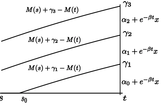
Figure 1: Situation in case A
• 0< γ1 < γ2 < . . . < γn,
• µs ≤0 for alls∈[t−ε, t] for someε >0.
We are going to prove this assertion by showing that if starting in situationAor B,V(t, x) again is of that type if time runs backward. In total we derive an algorithm which, starting
withV(T, x) (at timeT we are either in situationAorBdepending on the sign ofµT with
n= 0 and α0 = 0), constructs the whole value function and optimal strategy.
Proof: Assume µ(T)>0 or lim
t→Tsgn(µ(t)) = 1, i.e. we are in caseA.
LetM(t) = Rt
0 µr dr and ¯s= sup{s < t|µs<0} be the last time beforet where the drift changes its sign. Furthermore define
s0 = sup{s < t|M(s) +γ1−M(t) = 0},
s1 = sup{s < t|e−βs(M(s) +γ1−M(t)) +
Z t s
e−βrµrdr+α0 > e−βtγ1+α1}
= sup{s < t|
Z t s
µr(e−βr−e−βs)dr > γ1(e−βt−e−βs) +α1−α0}.
The point in times1 is the first time on the first curve (given by M(s) +γ1−M(t), going backward in time from t) where it is preferable to payout everything and consume the drift up to time t instead of staying there, reaching the point (t, γ1) where one receives
e−βtγ
1+α1. Figure 1 illustrates the specific situation of case A.
Lets∗= max{s, s¯ 0, s1}. At first we are going to look at the problem on the set:
where we assert that it is optimal to payout everything and to stay on the x-axis (i.e. consume the drift). This strategyC∗ is determined by:
∆Cs∗=Xs−,
˙
C∗
r =µr, r∈[s, t).
Assume from time s < t on we follow an arbitrary strategy C and switch to the optimal one at timet. Letτ = inf{r > s|XC
r <0} ∧t, we have
J(s, y, C) =
Z τ− s−
e−βr dCr+V(t, XtC−)I{τ=t}
=
Z τ− s−
e−βr(−dXrC+µr dr) +V(t, XtC−)I{τ=t} .
UsingN(s) =Rs
0 e−βrµrdr and integration by parts we derive
J(s, y, C) =N(τ)−N(s)−ne−βrXrC
r=τ− r=s−+β
Z τ s
e−βrXrC dro+V(t, Xt−)I{τ=t}
=N(τ)−N(s) +e−βsXsC−−e−βτXτC−−β
Z τ s
e−βrXrC dr (2)
+I{τ=t} e−βtXtC−+
n X
i=0
αiI[γi,γi+1)(X C t−)
!
.
Sinces≥s∗≥s0 the level γ1 can not be reached by XC, therefore (2) is equivalent to
J(s, y, C) =N(τ)−N(s) +e−βsXsC−−e−βτXτC−−β
Z τ s
e−βrXrC dr
+I{τ=t}
e−βtXtC−+α0
(3)
≤N(t)−N(s) +e−βsXsC−+α0 .
The last inequality is due to the fact thatN(·) is increasing. We observe that there is an equality in (3) for the above defined strategyC∗, which yields thatV(s, x) =e−βsx+α
0,new
withα0,new =α0+N(t)−N(s), i.e. V(s, x) is again of the claimed form.
Now we look at points{(s, x)|s∗ ≤s < t, x=M(s) +γ1−M(t)}, here the levelγ1 can be reached. Instead of (3) we have
N(τ)−N(s) +e−βsXsC−−β
Z τ s
e−βrXrC dr+I{τ=t, XC
t−<γ1}α0+I{τ=t, XtC−=γ1}α1 . (4) Suppose there is somer ∈[s, t] with XrC < M(r) +γ1−M(t), then at time tlevel γ1 can not be attained and (4) is smaller than
Whereas the policy staying on the curve, doing nothing, delivers the value e−βtγ
1+α1. Sinces≥s∗≥s1 the last policy yields a higher value such that
V(s, M(s) +γ1−M(t)) =e−βtγ1+α1, fors∗ ≤s < t .
As a first consequence we have thatV is not continuous along the curveM(s) +γ1−M(t). In a second step we deal with points which are in between the first curveM(s) +γ1−M(t) and the second oneM(s) +γ2−M(t). As we know from the above discussion it is optimal to stay on the first curve, in combination with Lemma 2.1 we obtain that it is not optimal
to jump from above this curve to a level below.
Define
s2 = sup{s < t|(γ2−γ1)e−βs+α1+e−βtγ1> α2+e−βtγ2}, (5)
which is the first time (going backwards fromt) such that it is as good to stay on the second curve as to jump down to the first curve and stay there. Actually this curve vanishes ins2 together with the associated discontinuity ofV.
Substituting the level x = 0 by the first curve in the previous step of the proof we obtain in an analogue way that fors≥s∗∨s2 if M(s) +γ1−M(t)< x < M(s) +γ2−M(t) it is
optimal to jump down to the first curve and stay there. Ifx is already on the second curve it is optimal to stay there up to timet.
An application of these thoughts to areas between higher curvesM(s) +γj −M(t) proves
the claimed structure ofV(s, x) and determines the optimal policy. In total we get withsk
k= 3, . . . , ndefined like s2 in (5):
• if for some index j we have sj > s¯, then the line of discontinuity given by M(s) +
γj−M(t) vanishes before a switch to case B
• if s0 > s¯, then the first line of discontinuity on the time axis vanishes (this may happen as well for the higher curves “later”, if these curves still exist.)
• in case µs≥0 the number of discontinuities can only decrease.
Figure 2: Situation in case B
¯
s= sup{s < t|µs>0},
s0 = sup{s < t|e−βs(M(s)−M(t))> α0},
s∗ = max{s0,s¯},
notices0 is the first point in time from tbackwards, where it is better to leave the lowest curveM(s)−M(t) by paying out everything instead of waiting until timet. The situation containing the curvesM(s) +γj−M(t) is illustrated in Figure 2.
We claim that on {(s, x)|s∗ ≤ s < t, 0 ≤ x < M(s)−M(t)} it is optimal to payout everything immediately. For an arbitrary strategyC we have as in caseA that:
J(s, x, C) =N(τ)−N(s) +e−βsXsC−−e−βτXτC−−β
Z τ s
e−βrXrC dr
+I{τ=t} e−βtXtC−+
n X
i=0
αiI[γi,γi+1)(X C t−)
!
. (6)
Sinces≥s∗ and x < M(s)−M(t) ruin happens before time t, therefore (6) is equal to
N(τ)−N(s) +e−βsXsC−−β
Z τ s
e−βrXrC dr≤e−βsXsC−.
The last equality holds since N(·) is decreasing, the “≤” changes to a “=” in the case everything is paid out immediately. ThereforeV(s, x) =e−βsx on {(s, x)|s∗ ≤s < t, 0≤
x < M(s)−M(t)}.
Figure 3: The first discontinuity curveγ1(s).
case (t,0) can be reached. We have
J(s, x, C) =N(τ)−N(s) +e−βsXsC−−e−βτXτC−−β Z τ
s
e−βrXrC dr+I{τ=t}α0. (7)
If there is some r ∈ [s, t] such that XrC < M(r) −M(t), one cannot reach (t,0) and
(7) is smaller or equal to e−βsXC
s . Staying on the curve gives the value α0. Because of
s≥ s∗ ≥ s0 this yields the higher value and V(s, M(s)−M(t)) =α0 for s∗ ≤ s < t. If
α0 >0 a discontinuity along M(s)−M(t) for s < tis generated in (t,0) which vanishes at times0.
The areas between the following higher curves can be treated as in caseA.
In the remark below we sum up some important properties of the value function following
from the above proof.
Remark 2.2
• If µ(T) > 0 or lim
t→Tsgn(µ(t)) = 1, then the value function is continuous on (s
∗, T]×
[0,∞), where s∗ = sup{s ∈ [0, T) : µs < 0}. On (s∗, T]×[0,∞) it is optimal to payout everything and the value function is given by
V(t, x) =e−βtx+ Z T
t
e−βsµ(s) ds .
In particular, the value function is continuous if µ(t)≥0 for all t∈[0, T]. (P4)
Assume s∗ >0 and α0(s∗) =RT
given by γ1(s) = −Rs
∗
s µr dr. In Figure 3 we see the functionM(s) = RT
s µr dr and the first discontinuity curve γ1(s) starting ins∗.
• The value function is right continuous in the x-component with
lim
h→0
V(t, x+h)−V(t, x)
h =e−
βt . (P5)
• There exist 0 = tm+1 < ... < t1 = T and continuously differentiable, either strictly
increasing or strictly decreasing functions
0< γ2,1 < ... < γ2,n2, ...,0 < γm+1,1 < ... < γm+1,nm+1 such thatV(t, x) is continuous on [0, T]×[0,∞)\S with S =
m+1
S j=2
nj S i=1{
(s, γj,i(s)), s∈ [tj, tj−1)}. Furthermore, V is
continuously differentiable in x on every set {(s, x) : tj < s < tj−1, γj,i−1(s)< x <
γj,i(s)}. (P6)
3
Dynamic programming - heuristics for Hamilton–Jacobi–
Bellman equation
As starting point for the derivation of some Hamilton–Jacobi–Bellman (HJB) equation we
need the following dynamic programming principle:
V(t, x) = sup
C∈C(t,x)
(
Z T¯∧τ− t−
e−βsdCs+V( ¯T ∧τ, XTC¯∧τ−)
)
, (8)
fort≤T¯≤T.
Proof: LetC ∈ C(t, x), then
J(t, x, C) =
Z τ−
t−
e−βsdCs+e−βτXτ
I{τ≤T¯}
+
Z T¯− t−
e−βsdCs+ Z τ−
¯
T−
e−βsdCs+e−βτXτ !
I{τ >T¯}
=
Z T¯∧τ− t−
e−βsdCs+J( ¯T ∧τ, XTC¯∧τ−, C),
where strategyC is taken for ¯T ≤s≤τ (just the Cfrom ¯T onwards). Therefore obviously we have:
V(t, x)≤ sup
C∈C(t,x)
(
Z T¯∧τ− t−
e−βsdCs+V( ¯T ∧τ, XTC¯∧τ−) )
Now setW(t, x) to be equal to the right hand side of (8) and let C∗ be anε/2>0 optimal strategy for it,
W(t, x)−ε 2 ≤
Z T¯∧τ− t−
e−βsdCs∗+V( ¯T ∧τ, XC
∗
¯
T∧τ−).
Since everything is deterministic we can choose again an ε/2 > 0 optimal strategy ¯C for ( ¯T∧τ, XTC¯∧∗τ−) such thatV( ¯T∧τ, XC
∗
¯
T∧τ−)−ε/2≤J( ¯T ∧τ, X
C∗
¯
T∧τ−,C¯). Then
W(t, x)−ε≤
Z T¯∧τC
∗
−
t−
e−βsdCs∗+
Z τC¯−
¯
T∧τC∗−
e−βsd ¯Cs+e−β(τ ¯ C
∧τC∗)
XC˜
τC¯∧τC∗
=J(t, x,C˜)≤V(t, x)
where XC˜ results from taking strategy C∗ form t to ¯T and if not ruined before going on with ¯C, i.e. ˜Cs =Cs∗I{t≤s<T¯}+ ¯CsI{T¯≤s≤T} and stopping it if ruin occurs. Therefore for
everyε >0 we have
W(t, x)−ε≤V(t, x)≤W(t, x),
which proves (8).
Now we can in a heuristic way derive the associated HJB equation. Suppose V(t, x) ∈
C1,1([0, T]×[0,∞)) and that C
s = Rs
t cz dz for some non-negative and continuous density
c: [t, T]→R+. LetC be an ε >0 optimal strategy forV(t, x) (x >0), then
V(t, x)−ε≤
Z t+h t
e−βscsds+V(t+h, x+ Z t+h
t
(µs−cs) ds
for √ε > h > 0 small enough such that x+Rt+h
t (µs−cs) ds ≥ 0. Applying a Taylor
expansion we get:
−ε≤he−βtct+h(Vt(t, x) + (µt−ct)Vx(t, x)) +o(h)
≤0.
Dividing byh we have
−√ε≤e−βtct+ (Vt(t, x) + (µt−ct)Vx(t, x)) +o(1)
≤0.
Takingh→0 indicates the following HJB equation for problem (1), 0 = maxe−βt−Vx(t, x), Vt(t, x) +µtVx(t, x)
, (9)
Since the optimal consumption strategy indicates that there are possible discontinuities of
V(t, x) in tand xwe may need to show that (9) is fulfilled in a viscosity sense.
Definition 3.1
The upper semi-continuous (usc) envelope ofV(t, x) is defined by
V∗(t, x) = lim sup (s,y)→(t,x) (s,y)∈[0,T]×[0,∞)
V(s, y), (t, x)∈[0, T]×[0,∞).
The lower semi-continuous (lsc) envelope ofV(t, x) is defined by
V∗(t, x) = lim inf (s,y)→(t,x) (s,y)∈[0,T]×[0,∞)
V(s, y), (t, x)∈[0, T]×[0,∞).
Definition 3.2
We say that a linearly bounded functionW : [0, T]×[0,∞)→R
• is a viscosity supersolution if for every ϕ∈C(1,1)[0, T]×[0,∞):
max{e−β¯t−ϕx(¯t,x¯), ϕt(¯t,x¯) +µ¯tϕx(¯t,x¯)} ≤0,
at every(¯t,x¯)∈(0, T)×(0,∞)which is a (strict) minimizer ofW∗−ϕon[0, T]×[0,∞)
with W∗(¯t,x¯) =ϕ(¯t,x¯).
• is a viscosity subsolution if for every ψ∈C(1,1)[0, T]×[0,∞):
max{e−β¯t−ψx(¯t,x¯), ψt(¯t,x¯) +µ¯tψx(¯t,x¯)} ≥0,
at every(¯t,x¯)∈(0, T)×(0,∞)which is a (strict) maximizer ofW∗−ψon[0, T]×[0,∞)
with W∗(¯t,x¯) =ψ(¯t,x¯).
W is a viscosity solution if it is both super- and subsolution.
Note: ψ≥W∗ ≥W ≥W∗ ≥ϕ.
Theorem 3.3
The functionV(t, x) given by (1)is a viscosity solution to (9).
For proof see Appendix.
To show the uniqueness of the value function we need the following Lemma, which indicates
Lemma 3.4
Forx∈[0,∞) we have
V∗(T, x) =V∗(T, x) =e−βTx .
For proof see Appendix.
Next we show the uniqueness of the value function. Since we are dealing with a
disconti-nuous value function, a classical Comparison Theorem common for the contidisconti-nuous case,
see for example Bardi and Capuzzo-Dolcetta [4] and references therein, cannot be applied.
Therefore, at first we show the uniqueness in the sense of weak comparison, i.e. we show
the uniqueness up to discontinuities. The usual technique to prove the uniqueness is to
compare the usc envelope u∗ of a subsolution u and the lsc envelope v∗ of a supersolution
v. Because we will be dealing only with continuity regions of the value function it holds
u=u∗ andv =v ∗.
Theorem 3.5
Letu be a sub- and v a supersolution to HJB Equation (9), having the properties (P1) – (P6) and fulfillingu(t, x)≤v(t, x)on{0}×[0, x]∪[0, T]×{0}. Then it holdsu(t, x)≤v(t, x)
onR, whereR:= [0, T]×[0,∞)\S withS defined in Remark 2.2.
For proof see Appendix.
Remark 3.6
Theorem 3.5 signifies the uniqueness of the value function in the regions, where it is
continu-ous. Due to Section 2 the value function has only finitely many discontinuities on[0, T]×{0}
and finitely many discontinuity curves, which are continuously differentiable functions of
time. Furthermore we know thatV(t, x) is right continuous in thex component. It is easy to see that the listed properties imply the uniqueness of the value function also on S.
4
Examples
In this section we consider two examples where we calculate the value function explicitly
cumbersome calculations, one can deal with the second one for which we just give the final
result and an illustrating plot.
Example 4.1
We choose T = 3π and set µt = sin(t) and β = 0.04, consequently M(t) = Rt
0 sin(s) ds. The value functionV fulfilsV(T, x) =e−βTx at (T, x).
Using the notation of Section 2 we have that:
γ0(0)= 0, γ1(0) =∞,n= 0,α(0)0 = 0 and sin(s)>0 on [3π−ε,3π).
Step 1:
Consider
¯
s(1) := sup{s≤3π: sin(s)<0}= 2π; Sinceγ1(0)=∞, we have s∗
1 = ¯s(1)= 2π.
On the set A0 := {(s, x) : 2π < s ≤ 3π, 0 ≤ x < ∞} it is optimal to payout the whole surplus immediately. Thus, we can give a closed expression forV(s, x) on the setA0:
V(s, x) = e−βsx+
Z T s
e−βrsin(r) dr
= e−βsx+ 1
β2+ 1
n
e−βscos(s) +βe−βssin(s) +e−βTo.
Now we are able to calculate the newγ- and α-functions: γ1(1) =∞ and
α(1)0 (s) = 1
β2+ 1
n
e−βscos(s) +βe−βssin(s) +e−βTo.
Step 2:
Fors∈[2π−ε,2π) it holds sin(s)<0 and we sett= 2π in the backward algorithm. Like above we calculates∗2 = 1.248846988π,γ1(2)(s) =M(s)−M(2π) = 1−cos(s). Observe that sinceα(1)0 (2π)>0 the point in time s∗2 is bigger than the next change of sign ofµt, i.e. the
discontinuity curveγ1(2)(s) vanishes at this point.
On the set A1 :={(s, x) :s∗2 ≤s <2π,0 ≤x < 1−cos(s)} we have, by the above results, that it is optimal to payout everything immediately, i.e. V(s, x) = e−βsx, which implies
α(2)0 = 0.
3,0 2,5 2,0 1,5 x 1,0 0
0
1 2 1
3 2
4
0,5
t 5 3
6 7 4
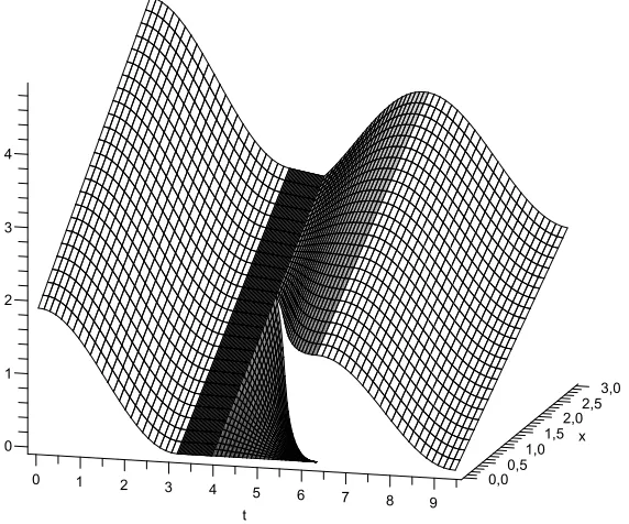
[image:16.595.159.445.62.300.2]8 9 0,0
Figure 4: The value function V(t, x) forµt= sin(t)
On the set {(s, x) : s∗2 ≤s < 2π, x ≥ 1−cos(s)} it is optimal to payout the difference to theγ1(2)-curve and to do nothing untilt= 2π.
Thus, we have V(s,1−cos(s)) = α(1)0 (2π) = e−βs(1−cos(s)) +α(2)
1 . Now it is easy to
calculate α(2)1 :
α(2)1 (s) : = α(1)0 (2π)−e−βs(1−cos(s))
= 1
β2+ 1
n
e−β2πcos(2π) +βe−β2πsin(2π) +e−β3πo
−e−βs(1−cos(s)).
AltogetherV(s, x) =e−βsx+α(2)1 (s) on{(s, x) :s∗2< s≤2π, x≥1−cos(s)}.
Step 4:
It holds sin(s)<0 in an ε environment of 1.248846988π. We calculate s∗3 =π, and obtain thatV(t, x) =e−βtxon {(s, x) :π ≤s <1.248846988π, 0≤x <∞}(in this area one pays
out everything and gets ruined!). Thereforeα(3)0 = 0 and γ1(3) =∞.
Step 5:
For 0≤s≤π we are in the same the situation like in the beginning of the example, with the consequence thatV(t, x) =e−βtx+e−βsx+β21+1
n
Summarizing the results and letting a:= e−β2π+e−β3π β2+1 yields
V(t, x) =e−βtx+I[0,π)(t) 1
β2+ 1
n
e−βtcos(t) +βe−βtsin(t) +e−βπo
+I[1.2488π,2π)×[1−cos(t),∞)(t, x)
n
a−e−βt(1−cos(t))o +I[2π,3π)(t)
1
β2+ 1
n
e−βtcos(t) +βe−βtsin(t) +e−β3πo.
In Figure 4.1 we see thatV(t, x) consists of 5 parts (which have different shadings). Each part corresponds to some dividend payout behaviour of the insurer, which are described in
Steps 1 – 5 above. The discontinuity region ofV(t, x) is given by
D:=
(t, x) : t∈[1.248846988π,2π) , x= 1−cos(t) .
One easily verifies thatV(t, x) fulfils (P1) – (P6) and solves the HJB equation (9).
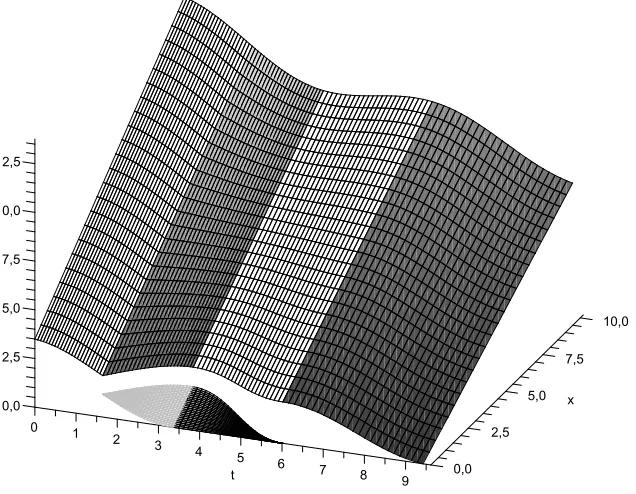
Example 4.2
In this example we consider the case where the drift function has a linear component
µt= sin(t) + 0.01t+ 0.2. Using the same algorithm like in Example 4.1, we obtain a closed
form expression for the value function, but calculations in this case are quite tedious.
Let
f(t, s) =
Z s t
(sin(r) + 0.01r+ 0.2)e−βr dr, g(t, s) =
Z s t
(sin(r) + 0.01r+ 0.2) dr.
Then the value function is given by:
V(t, x) =e−βtx+I[1.9162π,3π)(t)f(t,3π) +I[1.075π,1.9162π)(t)I[−g(t,1.9162π),∞)(x)
n
f(1.9162π,3π) +e−βtg(t,1.9262π)o +I[0.524π,1.075π)(t)I[0,−g(t,1.9162π))(x)f(t,1.075π)
+I[0.524π,1.075π)(t)I[−g(t,1.9162π),∞)(x)
n
f(1.9162π,3π) +e−βtg(t,1.9162π)o +I[0,0.524π](t)
n
f(t,0.524π) +f(1.9162π,2π))o.
The value function now consists of 6 parts, in Figure 4.2 they differ in shadings and
cor-respond to different types of strategies. The upper right, upper left and the both bottom
parts correspond to the strategy “payout everything”. The both top centre parts
10,0
7,5
5,0 x
0 0,0
1 2 3 2,5
t 4
2,5 5 6
5,0
7 8 9 7,5
0,0 10,0
[image:18.595.152.470.52.299.2]12,5
Figure 5: The value function V(t, x) forµt= sin(t) + 0.01t+ 0.2.
previous case it is easy to check that V(t, x) fulfils conditions (P1) – (P6) and solves the
HJB equation (9).
Appendix
HJB equation - viscosity solution
Proof of Theorem 3.3
We start with the supersolution proof (see the method in Mnif & Sulem [10]).
Letϕbe an appropriate test function and (t, x)∈(0, T)×(0,∞) such thatV∗(t, x) =ϕ(t, x) is a minimizer ofV∗−ϕ. Let{(tn, xn)} ⊂(0, T)×(0,∞) be a sequence with (tn, xn)→(t, x)
such thatV(tn, xn)→V∗(tn, xn) asn→ ∞. SinceV ≥V∗ ≥ϕwe have for a given strategy
Cn∈ C(t
n, xn) some small h >0 from (8):
ϕ(tn, xn)−ϕ(tn, xn) +V(tn, xn)≥
Z tn+h∧τn− tn−
e−βsdCsn+ϕ(tn+h∧τn, XC n
tn+h∧τn−).
(10)
We have by the choice of (tn, xn) that γn=V(tn, xn)−ϕ(tn, xn)→ V∗(t, x)−ϕ(t, x) = 0
and γn ≥ 0. If we chooseCsn =δ for s≥tn (one constant payment at time tn) for δ > 0
such thatXC
We obtain by sendingh→0 and n→ ∞:
ϕ(t, x)≥e−βtδ+ϕ(t, x−δ).
From which we get 0≥e−βt−ϕ x(t, x).
If we chooseCn
s = 0 for s≥tn we obtain from (10)
γn≥ϕ(tn+h∧τ, xn+
Z tn+h∧τ tn
µsds)−ϕ(tn, xn).
Since everything is deterministic we can takeh >0 small enough such thatxn+Rttnn+hµsds≥
0 for alln. A Taylor expansion gives
γn
h ≥ϕt(tn, xn) +µtnϕx(tn, xn) +o(1). (11)
If{γn}is equal to zero for only finitely manynwe take a strictly positive subsequence{γn}′
and chooseh=p
γ′
n and nlarge enough such that there is no ruin before tn+h.
If{γn} is equal to zero for infinitely many nwe take a subsequence {γn}∗ with γn∗ = 0 for
n∈N.
We get for (11) ifn→ ∞
0≥ϕt(t, x) +µtϕx(t, x),
which proves the supersolution property.
For proving the subsolution property we need to show:
For every ¯ψ∈C(1,1)[0, T]×[0,∞): max{e−β¯t−ψ¯
x(¯t,x¯),ψ¯t(¯t,x¯) +µ¯tψ¯x(¯t,x¯)} ≥0,
at every (¯t,x¯) ∈(0, T)×(0,∞) which is a (strict) maximizer of V∗−ψ¯ on [0, T]×[0,∞) withV∗(¯t,x¯) = ¯ψ(¯t,x¯).
As usual the subsolution proof is done via contradiction. Suppose there are some (¯t,x¯) and ¯
ψwith the properties stated before but with
max{e−β¯t−ψ¯x(¯t,x¯),ψ¯t(¯t,x¯) +µ¯tψ¯x(¯t,x¯)}<−2ξ , (12)
for someξ >0. Consider the function
ψ(t, x) = ¯ψ(t, x) + (x−x¯)
2+ (t−¯t)2 ¯
Then it holdsV∗(¯t,x¯) = ¯ψ(¯t,x¯) =ψ(¯t,x¯),ψ¯x(¯t,x¯) =ψx(¯t,x¯) and ¯ψt(¯t,x¯) =ψt(¯t,x¯) which
gives
max{e−β¯t−ψx(¯t,x¯), ψt(¯t,x¯) +µ¯tψx(¯t,x¯)}<−2ξ.
Becauseψ(t, x) is continuously differentiable in both tand xand µtis continuous, there is
δ∈(0,√¯t2+¯x2
2 ) such that
max{e−βt−ψx(t, x), ψt(t, x) +µtψx(t, x)}<−ξ
for (t, x)∈Bδ(¯t,x¯). We obtainV∗(t, x)≤ψ¯(t, x) =ψ(t, x)− δ 2
¯
t2+¯x2ξ for (t, x)∈∂Bδ(¯t,x¯).
Let nowε= 12 δ2
¯
t2+¯x2ξ, then onBδ(¯t,x¯) we have
max{e−βt−ψx(t, x), ψt(t, x) +µtψx(t, x)}<−ε , (13)
while for (t, x)∈/ Bδ(¯t,x¯) we have
V∗(t, x) =ψ(t, x)−2ε .
Now let (tn, xn)→(¯t,x¯) such thatV(tn, xn)→V∗(¯t,x¯) and assume (w.l.g.) that (tn, xn)∈
Bδ(¯t,x¯) for alln∈N.
LetCn∈ C(t
n, xn),XC n
be the corresponding wealth starting in (tn, xn) and τ∗ =τn∧T¯
(with some ¯T such thattn<T¯≤T for all n) where
τn= inf{s≥tn|XC n
s ∈/ Bδ(¯t,x¯)}.
At first we observeXCn
can only have downward jumps in thexdirection and thatV(t, x) is increasing inx. Because of continuity ofµt, jumps in the wealth process are due to jumps
in the consumption process and we haveXCn s −XC
n
s− =−∆Csn.
Supposeτ∗=τn, i.e. stopping because of leavingBδ(¯t,x¯). Then either we hit the boundary
continuously or leave the ball due to a jump at timeτ∗ in which caseXτ∗−∈Bδ(¯t,x¯). From the above estimates we get
V(τ∗, XCn
τ∗−)≤ψ(τ∗, XτC∗n−)−2εI{X
τ∗ −=Xτ∗}. Ifτ∗ = ¯T thenXCn
τ∗ as wellXτC∗n− as are still inside the ball and we have
V(τ∗, XCn
In total we arrive at
V(τ∗, XτC∗n−)≤ψ(τ∗, XC
n
τ∗−)−2εI{τn=τ∗∧X
τ∗−=Xτ∗}} =ψ(tn, xn) +
Z τ∗ tn
ψt(s, XC n
s ) +µsψx(s, XC n s ) ds −
Z τ∗− tn−
ψx(s, XC n
s ) dCsn,c+
X
tn≤s<τ∗, XsCn6=XsCn−
ψ(s, XsCn)−ψ(s, XsC−n)
−2εI{τn=τ∗∧Xτ∗−=Xτ∗} .
In the above formula Cn,cdenotes the continuous part of strategy Cn.
IfXCn s 6=XC
n
s− we have thatXC n s −XC
n
s− =−∆Csn and we can write X
tn≤s<τ∗, XsCn6=XsCn−
ψ(s, XsCn)−ψ(s, XsC−n) =− X
tn≤s<τ∗, XsCn6=XsCn−
Z ∆Cn s
0
ψx(s, x−α) dα
.
Combining the last expression with the continuous part ofCnand usinge−βt ≤ψ
x(t, x) on
Bδ(¯t,x¯) we arrive at
− Z τ∗−
tn−
ψx(s, XC n
s ) dCsn,c+
X
tn≤s<τ∗, XCns 6=XsCn−
ψ(s, XsCn)−ψ(s, XsC−n)
≤ − Z τ∗−
tn−
e−βsdCsn,c− X
tn≤s<τ∗, XsCn6=XCns−
e−βs∆Csn=−
Z τ∗− tn−
e−βsdCsn.
Finally usingψt(s, XC n
s ) +µsψx(s, XC n
s )≤ −εfrom (13) we get
V(τ∗, XτC∗n−) +
Z τ∗− tn−
e−βsdCsn+ (τ∗−tn)ε+ 2εI{τn=τ∗∧Xτ∗−=Xτ∗}≤ψ(tn, xn),
which is the same as
V(τ∗, XτC∗n−) +
Z τ∗− tn−
e−βsdCsn+ (τ∗−tn)ε+ 2εI{τn=τ∗∧Xτ∗−=Xτ∗}≤ψ(tn, xn)
≤V(tn, xn) + (ψ(tn, xn)−V(tn, xn)).
Since alsoψ(tn, xn)→V∗(¯t,x¯) if n→ ∞ we can choosenlarge enough such that
0≤ψ(tn, xn)−V(tn, xn)≤
(τ∗−tn)ε+ 2εI{τn=τ∗∧Xτ∗−=Xτ∗}
2 .
We get
V(τ∗, XτC∗n−) +
Z τ∗− tn−
e−βsdCsn+(τ
∗−tn)ε+ 2εI
{τn=τ∗∧Xτ∗−=Xτ∗}
Now before we can state that (14) is a contradiction to (8). We have to discuss the case
τ∗ = τn =tn, where an immediate lump-sum consumption leads to xn = XCn
τ∗− > XC
n τ∗ ∈/
Bδ(¯t,x¯). We notice that property (P6) and the construction of the value function show
that in this caseV is continuously differentiable around the point (¯t,x¯) andVx(¯t,x¯) =e−β¯t.
Therefore V∗ = V around (¯t,x¯) which furthermore yields that ψx(¯t,x¯) =e−β¯t. Since the
test functionψis continuously differentiable inx, inequality (13) can not be true and states a contradiction to (12).
Thus we have, when stating (12), that there exists an area around (¯t,x¯) inside which it is not optimal to consume a lump sum from the wealth. Consequently a strategy Cn, for
playing a role in the dynamic programming principle forn large enough such that (tn, xn)
are inside this non-paying area, has the feature thatXCn
t can leaveBδ(¯t,x¯) through a jump
not before leaving the non-paying area continuously.
Thereforeτ∗> tn, which completes the proof and we can conclude thatV(t, x) is a viscosity
solution to (9).
Proof of Lemma 3.4
SinceV(t, x) ≥e−βtx for (t, x)∈[0, T]×[0,∞) (you can always payout everything andquit
by consuming a small constant rate such thatXt+<0) we also have
V∗(t, x)≥e−βtx , V∗(t, x)≥e−βtx .
From e−βTx=V(T, x)≥V∗(T, x) we getV∗(T, x) =e−βTx. Assume thatV∗(T, x)> e−βTx, then there exists some η >0 with
V∗(T, x)≥2η+e−βTx .
Now choose a sequence (tn, xn) → (T, x) such that V(tn, xn) → V∗(T, x). There is some
n0>0 such that forn≥n0 we have
V(tn, xn)≥η+e−βTx . (15)
Let Cn ∈ C(t
n, xn) and define τn = inf{t ≥ tn|XC n
t < 0} ∧T. Since Cn is admissible
we have ∆Cn
definition of tn we have τn−tn → 0 if n → ∞. Now fix some ε > 0 and choose n large
enough such that
Z τn− tn−
e−βr dCrn+e−βτnXCn τn− ≤e
−βtnCn tn+e
−βtn(x
n−Ctnn) +ε=e
−βtnx n+ε .
Taking a supremum over strategies Cn we get V(t
n, xn) ≤ e−βtnxn+ε which contradicts
(15) sinceεis arbitrary and if (tn, xn)→(T, x) we havee−βtnxn→e−βTx.
Proof of Theorem 3.5:
Assume there is (ˆt,xˆ)∈R such that u(ˆt,xˆ)−v(ˆt,xˆ)>0. W.l.o.g. we assume ˆt∈[tj, tj−1) and ˆx ∈ γj,i(ˆt), γj,i+1(ˆt)
with tj < tj−1, γj,i < γj,i+1 defined as in Section 2 and in Remark 2.2. We also assume, that the comparison principle is already shown for the
intervals [tl, tl−1) with l ∈ {j−1, ..., m}, i.e. u(t, x) ≤v(t, x) on [tj, T]×R+. Note that Lemma 3.4 yieldsu(x, T) =v(x, T) for all x∈R+.
Define vk = kv for k > 1. It is easy to check, that kv˜ is still a supersolution with lsc envelopekv. Choosek > 1 such that u(ˆt,xˆ)−vk(ˆt,xˆ) >0. Due to Lemma 1.1 we obtain
the following inequality:
u(t, x)−vk(t, x) =u(t, x)−kv(t, x)≤xe−βt(1−k) +λ(t)
≤xe−βtj−1(1
−k) +λ(0) =:η .
It is clear that u(t, x)−vk(t, x) ≤ 0 for x ≤ λk(0)−1eβtj−1 =: η. If γ
j,i+1 = ∞ on [tj, tj−1) consider
A:={(t, x) :tj ≤t < tj−1, γj,i(t)< x < η}.
Ifγj,i+1<∞ on [tj, tj−1) consider
A:={(t, x) :tj ≤t < tj−1, γj,i(t)< x < γj,i+1(t)}.
W.l.o.g. we assume γj,i+1(t) < ∞ on [tj, tj−1) and γj,l(t), l ∈ {1, ..., nj}, increasing on
[tj, tj−1).
Note that due to properties (P5) and (P6) the function u(t, x)−vk(t, x) is continuously differentiable and decreasing on A. In particular, ˆx≥γj,1(ˆt).
Define further
M := sup (t,x)∈A{
From above we know thatM < λ(0)<∞ and obtain
0< u(ˆt,xˆ)−vk(ˆt,xˆ)≤M .
Since u−vk is continuous on A there is (t∗, x∗) ∈A withu(t∗, x∗)−vk(t∗, x∗) > M
2 >0. Define furtherH :={(t, x, s, y) : (t, x) ,(s, y)∈A, y−x ≥0, t−s≥0}, m:= k2 and for
ξ >0:
fξ(t, x, s, y) =u(t, x)eβs−vk(s, y)eβt−
ξ
2(x−y) 2
−nξ2(y 2m
−x+t−s) +ξ +
1 (x−γj,i(t))ξ
+ 1
(γj,i+1(s)−y)ξ
o
.
Then it holds
fξ(t, γj,i(t), s, y) =fξ(t, x, s, γj,i+1(s)) =−∞
for (t, γj,i(t), s, y),(t, x, s, γj,i+1(s)) ∈ H¯. Note that (t, x, s, γj,i(s)),(t, γj,i+1(t), s, y) ∈ H only ift=s, which yields fξ(t, x, s, γj,i(s)), fξ(t, γj,i+1(t), s, y)<0.
Let Mξ = sup H
fξ. Because fξ is continuous on H there is (tξ, xξ, sξ, yξ) ∈ H¯ such that
Mξ =fξ(tξ, xξ, sξ, yξ). Since (t∗, x∗) ∈A, it holds γj,i(t∗)< x∗ < γj,i+1(t∗), from which it follows
Mξ ≥fξ(t∗, x∗, t∗, x∗) = u(t∗, x∗)−vk(t∗, x∗)
eβt∗−2m ξ
− (γ 1
j,i+1(t∗)−x∗)ξ −
1 (x∗−γj,i(t∗))ξ
> M
2 e
βt∗
−2ξm −(γ 1
j,i+1(t∗)−x∗)ξ −
1
(x∗−γj,i(t∗))ξ .
We obtain directly
Mξ >0 for ξ >4
2m+ 1/(x∗−γj,i(t∗)) + 1/(γj,i+1(t∗)−x∗)
M et∗ =:ξ0 lim inf
ξ→∞ Mξ ≥
M
2 >0.
The boundary ofH is given by
∂H = {(t, x, s, y) : (t, x)∈A ,(s, y)∈∂A , s < t , x < y}
∪ {(t, x, s, y) : (t, x)∈∂A ,(s, y)∈A , s < t , x < y}
∪ {(t, x, s, y) : (t, x),(s, y)∈A , s¯ ≤t , x=y}
∪ {(t, x, s, y) : (t, x),(s, y)∈A , s¯ =t , x < y}. (16) Let us first consider the boundary of the set A:
∂A = {(t, γj,i+1(t)) : t∈[tj, tj−1]} ∪ {(t, γj,i(t)) :t∈[tj, tj−1]}
∪ j [
l=j−1
{(tl, x) : x∈[γj,i(tl), γj,i+1(tl)]}.
Consider the first two sets. By the construction of fξ and ¯H it holds fξ(t, x, s, y) < 0 if
x∈ {γj,i+1(t), γj,i(t)} or y∈ {γj,i+1(s), γj,i(s)}.
For tl = tj−1 it holds fξ(tj−1, x, s, y), fξ(t, x, tj−1, y) ≤ 0 by the assumption u(t, x) −
vk(t, x)≤0 on [t
j−1, T]×R+.
It remains to considertl=tj. We have
d
dyfξ(t, x, s, y) =−ke
βte−βs
−ξ(y−x) + 2m
ξ(y−x+t−s) + 12 −
1
(γj,i+1(s)−y)2ξ
≤ −k−ξ(y−x) + 2m− 1
(γj,i+1(s)−y)2ξ ≤ 0.
That is, fξ(t, x, s, y) is decreasing in y. Also it holds
d
dxfξ(t, x, s, x) =e−
β(t−s)−keβ(t−s)+ 1
(x−γj,i(t))2ξ −
1
(γj,i+1(s)−x)2ξ
≤1−k+ 1 (x−γj,i(t))2ξ
.
Since fξ(t, γj,i(t), s, y) = −∞ and fξ continuous there is δ > 0 for all t ∈ [tj, tj−1] s.t.
fξ(t, x, s, y) ≤ 0 for x−γj,i(t) < δ. In other words fξ(t, x, s, x) is decreasing in x for
x−γj,i(t) ≥ δ and ξ > δ2(k1−1). Since t ≥ s and y ≥ x it holds (tj, x, s, y) ∈ H¯ ⇒
(tj, x, s, y) = (tj, x, tj, y), which gives
fξ(tj, x, s, y) =fξ(tj, x, tj, y)≤fξ(tj, x, tj, x)
≤
fξ(tj, γj,i(tj), tj, γj,i(tj))<0 : x−γj,i(tj)≥δ
0 : otherwise
On the other hand because the functionsγj,i, γj,i+1 are increasing it holds
(t, x, tj, y)∈H¯ ⇒γj,i(t)≤x ≤y≤γj,i+1(tj),
and we can conclude like abovefξ(t, x, tj, y)≤0.
Now we know that (tξ, xξ, sξ, yξ)∈H\∂H forξ >max{ξ1, ξ0},ξ1:= δ2(k1
−1).
Note further that it holds
fξ(tξ, xξ, sξ, xξ) +fξ(tξ, yξ, sξ, yξ)≤2fξ(tξ, xξ, sξ, yξ).
Choose now a sequenceξn→ ∞ such that (tξn, xξn, sξn, yξn) →(¯t,x,¯ s,¯ y¯). From above we
obtain
ξn
(xξn−yξn)
2
≤u(tξn, xξn)e βsξn
−u(tξn, yξn)e βsξn
+vk(sξn, xξn)e βtξn
−vk(sξn, yξn)e βtξn
− yξn−xξn
(xξn−γj,i(tξn))(yξn−γj,i(tξn))ξ − yξn−xξn
(γj,i+1(sξn)−xξn)(γj,i+1(sξn)−yξn)ξ
+ 4m(yξn−xξn)
ξn(tξn−sξn) + 1
ξn(yξn−xξn+tξn−sξn) + 1
≤ −e−β(tξn−sξn)+keβ(tξn−sξn)
(yξn−xξn)
+ 4m(yξn−xξn)
ξn(tξn−sξn) + 1
ξn(yξn−xξn+tξn−sξn) + 1
. (17)
It is obvious that the right hand side is bounded. Then the left hand side is bounded as
well, which is possible only if (xξn−yξn)
2 →0 asn→ ∞. We conclude ¯x= ¯y. Taking now the limits on the both sides in (17) yields
lim
n→∞ξn(xξn−yξn) 2 ≤0,
which impliesξn(xξn−yξn)
2 →0. Also we obtain immediately
0≤ lim
ξn→∞
ξn(yξn−xξn)≤ −e−
β(tξn−sξn)−keβ(tξn−sξn)
+ 4m
ξn(tξn−sξn) + 1
ξn(yξn−xξn+tξn−sξn) + 1
Note thatξn(tξn−sξn)→ ∞implies lim ξn→∞
ξn(yξn−xξn)<0, which is a contradiction. Thus,
we conclude lim
ξn→∞
ξn(tξn−sξn)<∞, from which it follows ¯t= ¯sand ξn(tξn−sξn)
2 →0.
Note that ¯x is bounded away from γj,i+1(¯t) andγj,i(¯t).
Define the functions
ψ(t, x) =nξn
2 (x−yξn)
2+ 2m
ξ2
n(yξn−x+t−sξn) +ξn
+ 1
(x−γj,i(t))ξn o
+vk(sξn, yξn)e
βt+ 1
(yξn−γj,i+1(sξn))ξn
+Mξn ,
φ(s, y) = −nξn
2 (xξn−y)
2+ 2m
ξ2
n(y−xξn+tξn−s) +ξn
+ 1
(xξn−γj,i(tξn))ξn o
+u(tξn, xξn)e
βs− 1
(y−γj,i+1(s))ξn −
Mξn.
These functions are continuously differentiable in t and in x. Furthermore u(t, x)eβsξn −
ψ(t, x) attains its maximum at (tξn, xξn); v
k(s, y)eβtξn
−φ(s, y) attains its minimum at (sξn, yξn). Thus, ψ(t, x)e−
βsξn and φ(s, y)e−βtξn are test functions for u(t, x) and vk(s, y)
respectively. From
lim
n→∞ψx(tξn, xξn) = limn→∞φy(sξn, yξn) = 2m =k , (18)
we conclude that there isN ∈Nsuch that forn > N it holds
e−βtξn −ψx(t
ξn, xξn)e− βsξn
≤0, e−βsξn −φx(s
ξn, yξn)e− βtξn
≤0.
Therefore it holds by Definition 3.2 of viscosity sub- and supersolutions:
0 ≥ φs(sξn, yξn) +µsξnφy(sξn, yξn),
0 ≤ ψt(tξn, xξn) +µtξnψx(tξn, xξn).
Subtracting the above inequalities, rearranging the terms and letting ξn → ∞ yields the
following relation
lim
n→∞(u(tξn, xξn)−v k(s
ξn, yξn))≤0.
On the other hand we know
0< M
2 ≤lim infξ→∞ Mξ ≤nlim→∞Mξn = limn→∞(u(tξn, xξn)−v k(s
ξn, yξn)),
References
[1] Avanzi, B. (2009). Strategies for dividend distribution: A review. North American Actuarial Journal
13, 217 – 251.
[2] Albrecher, H. and Thonhauser, S. (2009). Optimality results for dividend problems in insurance.
Revista de la Real Academia de Ciencias Exactas, F´ısicas y Naturales. Serie A. Matem´aticas. RACSAM
103(2), 295 – 320.
[3] Barron, E.N. and Jensen, R. (1990). Semicontinuous viscosity solutions for Hamilton-Jacobi equations
with convex Hamiltonians.Communications in Partial Differential Equations15 (12), 293 – 309.
[4] Bardi, M. and Capuzzo-Dolcetta, I. (1997). Optimal Control and Viscosity Solutions of Hamilton–
Jacobi–Bellman Equations. Birkh¨auser, Boston.
[5] Cox J.C. and Huang C.F. (1989) Optimal consumption and portfolio policies when asset prices follow
a diffusion process.Journal of Economic Theory 49, 33 – 83.
[6] Fleming, W.H. and Soner, H.M. (1993).Controlled Markov Processes and Viscosity Solutions.
Springer-Verlag, New York.
[7] Grandits, P. (2009). Optimal consumption in a Brownian model with absorption and finite time
hori-zon.Preprint, 1 – 31.
[8] Karatzas I., Lehoczky J.P., Sethi S.P. and Shreve S.E. (1986). Explicit solution of a general
consump-tion/investment problem.Mathematics of Operations Research11, 261 – 294.
[9] Karatzas I., Lehoczky J.P. and Shreve S.E. (1987). Optimal portfolio and consumption decisions for a
“small investor” on a finite horizon.SIAM Journal of Control and Optimization 25, 1157 – 1186.
[10] Mnif, M. and Sulem, A. (2005). Optimal risk control and dividend policies under excess of loss
rein-surance.Stochastics 77(5), 455 – 476.