Bedford, T.J. and Denning, Richard and Revie, Matthew and Walls, Lesley (2008) Applying Bayes Linear Methods to Support Reliability Procurement Decisions. Working Paper. University of Strathclyde. (Unpublished)
http://strathprints.strath.ac.uk/7452/
Strathprints is designed to allow users to access the research output of the University of Strathclyde. Copyright © and Moral Rights for the papers on this site are retained by the individual authors and/or other copyright owners. You may not engage in further distribution of the material for any profitmaking activities or any commercial gain. You may freely distribute both the url (http://eprints.cdlr.strath.ac.uk) and the content of this paper for research or study, educational, or not-for-profit purposes without prior permission or charge. You may freely distribute the url
(http://eprints.cdlr.strath.ac.uk) of the Strathprints website.
Applying Bayes Linear Methods to Support Reliability Procurement Decisions
Tim Bedford, Richard Denning, Matthew Revie *, Lesley Walls
* Corresponding Author
Department of Management Science
Strathclyde Business School
University of Strathclyde
40 George Street
Glasgow
G1 1QE
Email: [email protected]
[email protected]
[email protected]
M
M
M
a
a
a
n
n
n
a
a
a
g
g
g
e
e
e
m
m
m
e
e
e
n
n
n
t
t
t
S
S
S
c
c
c
i
i
i
e
e
e
n
n
n
c
c
c
e
e
e
2
ABSTRACT
Bayesian methods are common in reliability and risk assessment, however, such methods often demand a large amount of specification and can be computationally intensive. Because of this, many practitioners are unable to take advantage of many of the benefits found in a Bayesian-based
approach. The Bayes linear methodology is similar in spirit to a Bayesian approach but offers an alternative method of making inferences. Bayes linear methods are based on the use of expected values rather than probabilities, and updating is carried out by linear adjustment rather than by Bayes Theorem. The foundations of the method are very strong, based as they are in work of De Finetti and developed further by Goldstein. A Bayes linear model requires less specification than a corresponding probability model and for a given amount of model building effort, one can model a more complex situation quicker. The Bayes linear methodology has the potential to allow us to build ``broad-brush" models that enable us, for example, to explore different test setups or analysis methods and assess the benefits that they can give. The output a Bayes linear model is viewed as an approximation to
``traditional" probabilistic models.
The methodology has been applied to support reliability decision making within a current United Kingdom Ministry of Defence (MOD) procurement project. The reliability decision maker had to assess different contractor bids and assess the reliability merit of each bid. Currently the MOD assess reliability programmes subjectively using expert knowledge - for a number of reasons, a quantitative method of assessment in some projects is desirable. The Bayes linear methodology was used to support the decision maker in quantifying his assessment of the reliability of each contractor's bid and determining the effectiveness of each contractor's reliability programme. From this, the decision maker was able to communicate to the project leader and contractors, why a specific contractor was chosen.
The methodology has been used in other MOD projects and is considered by those within the MOD as a useful tool to support decision making. The paper will contain the following. The paper will introduce the Bayes linear methodology and briefly discuss some of the philosophical implications of adopting a Bayes linear methodology within the context of a reliability programme analysis. The paper will briefly introduce the reliability domain and the reasons why it is believed that the Bayes linear methodology can offer support to decision makers. An in-depth analysis of the problem will then be given documenting the steps taken in the
project and how future decision makers can apply the methodology. A brief summary will then be given as to possible future work for those interested in the Bayes linear methodology.
Keywords:
Bayes Linear Methods, Risk Assessment, Reliability Procurement, Sensitivity Analysis
1. INTRODUCTION
The Bayes linear methodology is a quantitative method to express subjective beliefs and to review these beliefs once observations have been made [1]. An in-depth summary of the Bayes linear methodology can be found in [2]. It is an inferential tool that is similar in philosophy to “traditional" probabilistic Bayesian methods, but has a number of distinct features which give it certain advantages over these approaches when modeling complex problems [3]. Whilst “traditional" Bayesian approaches are demanding in terms of time, computational and elicitation effort, the Bayes linear methodology offers a quick and simple method to perform inference using expectation rather than probability as a basis. As such, the elicitation specification required from a decision maker is reduced and hence more complex scenarios can be modeled for an equivalent amount of resources.
One motivation for using Bayes linear inference is therefore a practical one – to extend the scope of analysis to tackle challenging problems that previously would have been unfeasible or too costly using a ``traditional" Bayesian approach. We use Bayes linear methods to focus on a decision maker's subjective beliefs about some uncertain quantities. When modeling a problem, we assume that a decision maker holds certain beliefs about some quantities of interest (i.e. the MTBF of a system) and that the decision maker is able to make observations (i.e. the MTBF of a previous system) that they believe are related in some way (i.e. the MTBF of previous system is 50 hours less than the MTBF of the new system) to the original quantity of interest. The prior beliefs about these uncertain quantities are then linearly adjusted based on the information gathered and the Bayes linear formulas. Examples of practical complex problems modeled using BL methods are [4], [5], and [6].
The main difference between conventional probabilistic Bayesian methods and Bayes linear revolves around how beliefs about uncertain quantities are specified. Expectations are used as a primitive, rather than probability, following the development of de Finetti [7]. In the Bayes linear framework, a decision maker's uncertainty is represented by variance. The variance represents the decision maker's degree of uncertainty in specifying the exact value of a given variable. Whereas “traditional" Bayesian approaches use joint probability distributions to model relationships between quantities, Bayes linear uses covariance. The covariance quantifies the extent to which one quantity influences our belief about another quantity. For information on how these quantities are elicited from experts, see [6], [8], [9], [10] and in particular, [11].
With the support of the United Kingdom Ministry of Defence (MOD), the Bayes linear method has been used to support reliability decision making on two ‘live’ projects. This paper focuses on one of these projects and shows how the Bayes linear methodology has been used to support decision making. The construction of a Bayes linear model comprises three parts. First, we need to structure the model. Second, we need to populate the model with our decision maker's beliefs. Finally, we must analyze the model once observed data has become available. This paper will briefly discuss how this has been carried out. For a more detailed description of all the steps, see [11].
2. Bayes Linear Theory
also specify cov(X, D). This matrix must be non-negative definite. One can represent D
as D = αX + R where R represents the unexplained uncertainty between X and D. Once these values are elicited and observations made, the decision maker can use the following formulae to adjust their prior assessments by linear fitting. The adjusted expectation of X given observation of a collection of quantities D written ED(X) is ED
(X) = E(X) + cov(X, D) var-1(D) (D-E(D)) where var-1(D) is the Moore-Penrose generalized inverse. Variance is used to quantify uncertainty. The adjusted variance of X
given D is var(D) = var(X) – cov(X,D)var(D)cov(D,X)
An important part of any inference is how the output of the model is interpreted by decision makers. For a detailed description of the different interpretations of the Bayes linear output, see [2]. For the purposes of this project, the adjusted quantities are interpreted as follows; ED(X) is viewed as an intuitive numerical summary of our
subjective beliefs of X given the observations D, i.e. an approximate estimator for X. VarD(X) is viewed as a strict upper bound on the expected posterior variance. In some
special cases, this may in fact be an exact value for the expected posterior expectation and variance. One such special case is when the joint probability distribution between X
and D is multivariate normal [2]. Hence, it seems reasonable to assume that if the decision maker believes that the uncertain quantities are approximately joint normally distributed, then the posterior belief structure is approximately normal distributed.
Bayes linear networks are used in a similar way to Bayesian Belief Networks. In a Bayes linear network, a node represents an uncertain variable whilst an arc represents the potential for a source node to influence the decision maker's belief about the destination node. In the Bayes linear network, an arc does not necessarily represent a causal relationship but instead it represents the fact that the value of one variable influences a decision maker's belief about the value of another variable. Figure 1 is the Bayes linear network for D = αX + R.
X D
Figure 1 – Bayes linear network for X and D
3. Elicitation
For a Bayes linear model with variables (X1, … , Xn), to populate the model it is necessary to elicit E(Xi) for i =1, … ,n and cov(Xi, Xj) for i,j = 1, … , n. Eliciting means and covariances directly can often be difficult as experts do not naturally think in these terms. Methods have been developed which focus on eliciting percentiles and then calculating the mean and variance of the variable directly. Pearson and Tukey [12] suggested a method specifically for the mean and variance which uses 3 percentiles for the mean and 5 for the variance. Keefer and Bodily [13] further developed this method for eliciting the variance so that the analyst was only required to specify 3 percentage points. This technique, referred to as the Pearon and Tukey method throughout this paper, was used in order to elicit the necessary means and variance values.
Due to the way in which prior beliefs are specified in a Bayes linear framework, there are a limited number of ways in which the dependency value between two variables can be specified. For this project, two different methods were used. As the Bayes linear methodology assumes that the relationship between any two variables can be written such that D = αX + R, one method of eliciting the covariance is for the decision maker to specify α, E(X), var(X), E(R) and var(R) using the Pearson and Tukey method. From
this, cov(X,D) = αvar(X).
An alternative method is for the decision maker to state E(X), var(X), E(D) and var(D) using the Pearson and Tukey method. From this, the decision maker is asked to consider the effect of observing D = d on their belief regarding E(X). Rearranging the Bayes linear formulas, cov(X,D) can be calculated.
Whilst the Bayes linear methodology offers an alternative to Bayesian Belief Networks and overcomes some of its weaknesses, the Bayes linear methodology also has some limitations. One of the strengths of the Bayes linear theoretical framework is that it does not require the decision maker to specify a distributional form for the uncertain variables that they are attempting to model. As Bayes linear only requires the decision maker to specify his or her first two moments, it does not distinguish between symmetric and skewed variables. One method around this problem would be to specify and model higher moments, such as X2. A further limitation of the Bayes linear methodology is that the adjusted variance is always less than the original variance once an observation has been made regardless of what is observed. As can be seen from the formula for the adjusted variance, as var-1(D) > 0 and cov2(X, D) ≥0, then the adjusted variance must always be less than or equal to the original variance. This might not be satisfactory for all cases, however, this is also the case for the binomial/beta Bayesian models which is commonly used in Bayesian reliability analysis.
A final limitation of the Bayes linear methodology is that it does not allow for easy modeling of quantiles. This is because no distributional form is assumed on the uncertain variables. Because of this, the information being fed back to the decision maker from the output of the model is not as detailed as the Bayesian Belief Network methodology. The Bayes linear approach may be looked upon as a quick and simple methodology that approximates a full detailed probabilistic analysis and can potentially be used when the resources for a full analysis are unavailable. Ultimately, it should be viewed as a method to approximate the traditional ‘traditional’ Bayesian approach. However, it offers a logical and justifiable framework to handle problems in which it may only be possible to elicit partially specified beliefs.
4. Project Background
The MOD is procuring two land vehicles within a single procurement project. Both vehicles are individually designed and built, however, there are a number of sub-systems common to both vehicles. These include the hydraulic systems, power, electrical systems, suspension and other major sub-systems. In addition, the reliability programme and analysis for both vehicles are being carried out by a single contractor. The contracted reliability requirement for each vehicle is measured as both a basic reliability and mission reliability. Basic (or mission) reliability is defined as the probability the vehicle will complete a battlefield mission (BFM) without a basic (or mission) failure occurring. The reliability requirement for mission reliability for Vehicle A is 0.55 and for Vehicle B, 0.57. The reliability requirement for basic reliability is 0.24 for Vehicle A and 0.26 for Vehicle B (The data has been changed to maintain confidentiality). Both vehicles are purposely built to carry out tasks currently undertaken by vehicles that have been modified. Based on previous experience, these reliability requirements will be challenging to achieve, but not unrealistic.
been met. The contractor planned to carry out 30 BFM for Vehicle A split into three phases with 10 in each. Similar plans were made for Vehicle B. Based on the evidence provided by the contractor, the MOD decision maker must assess whether or not either vehicle will meet, or has already met, their basic and mission reliability requirements. The single source of evidence presented at this time is the output of the RGT's. In order to determine whether or not either vehicle will meet their respective requirements, the MOD decision maker is interested in the current reliability of each vehicle and using his subjective engineering judgment, he will assess whether or not he believes each vehicle is likely to improve by the required amount needed to meet the requirement.
5. Project Modelling
The purpose of the modeling is to develop a high-level methodology capable of assessing the basic and mission reliability of Vehicle A and Vehicle B using the observed data gathered during the reliability growth trial (RGT) and expert assessment of the expected growth between different phases of the RGT's. The aim is to highlight to the decision maker at the earliest possible stage, whether or not the in-service basic or mission reliability of Vehicle A or Vehicle B is likely to be met. The modeling will also attempt to capture a number of softer factors that are not addressed by other statistical methods.
Each vehicle was being subjected to 10 BFM during three different phases. It was assumed that the basic and mission reliability of each vehicle could be estimated using the data gathered during the phase. The value gathered using the RGT phase data and US Army Material Systems Analysis Activity
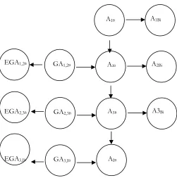
(AMSAA) calculations is the value that will be used to assess the current reliability of each variant of each system. The basic reliability of Vehicle A prior to Phase 1 of the RGT is A1B and the observed basic reliability of Vehicle A during Phase 1 is A1Bi. Similar notation is used for Phase 2, 3 and the in-service variation of the vehicle. In addition to the observed phase data, the MOD decision maker believed that he could gather additional information from the contractor prior to each phase regarding the expected reliability growth between the phases. For example, GA1,2B is the basic reliability growth of Vehicle A between phase 1 and 2 whilst EGA1,2B is the value specified by the contractor’s expert regarding this growth.
From this information, we can build a Bayes linear network for Vehicle A’s basic reliability.
A1Bi A1B
Figure 2 – Bayes linear network for Vehicle A’s basic reliability
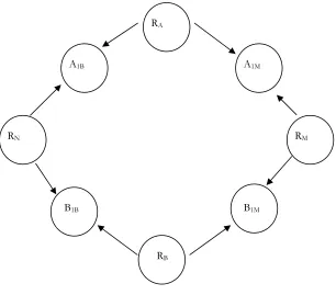
The decision maker also specified that he believed that learning about the basic (or mission) reliability of Vehicle A informed him about the mission (or basic) reliability of Vehicle A, and similarly for Vehicle B. In addition, he believed that learning about the Vehicle A’s basic reliability, informed him about the basic reliability of Vehicle B, and similarly for mission reliability. As such Figure 2 must be extended to take this information into account. Due to space restrictions, Figure 3 is only partially extended. For the full Bayes linear network, see [11].
6. Elicitation
A short example will be given to show the style of questions asked of the decision maker on the project. In order to elicit the basic reliability of Vehicle A prior to phase 1, the decision maker was asked “What is your belief about the 5, 50 and 95 percentiles of the basic
reliability of the Vehicle A's system entering Phase 1 of the RGT?” Based on the decision maker’s
response, E(A1B) and var(A1B) can be calculated.
To elicit the variance of the observations, the decision maker was asked “If you knew for certain the basic reliability of Vehicle A prior to Phase 1 was 0.1, what is your 5, 50 and 95 percentiles for the output of the vehicle during phase 1?” From this, E(A1Bi) and var(A1Bi) can be calculated.
To elicit the covariance between Vehicle A’s basic reliability and Vehicle B’s basic reliability, the decision maker was asked “Given that you know for sure basic reliability of Vehicle A prior to phase 1 is 0.1, what is your new belief about the expectation of Vehicle B's basic reliability
prior to phase 1?” Using the decision maker’s response and rearranging the Bayes linear
equations, cov(A1B, BB1B) can be calculated.
B
A2Bi A2B
A3Bi A3BB
GA1,2BB
EGA1,2B
GA2,3BB
GA3,IBB AIBB
B
EGA2,3BB
RA
[image:9.595.122.428.63.332.2]A1M
Figure 3 – Bayes linear network for Vehicle A and B’s basic and mission reliability
7. Analysis
Due to timing and access of data, the model has been built and populated with the decision maker's subjective beliefs, however, all the necessary observations to carry out inference on the reliability parameters of interest has not been gathered. Table 1 shows the initial belief of the decision maker.
Variable Expectation Standard Deviation
AIB 0.285 0.057
AIM 0.584 0.128
BBIB 0.302 0.061
BBIM 0.578 0.118
Table 1 – Prior belief
Prior to any observations being made, the decision maker believes all reliability requirements will be met. However, there is still substantial uncertainty in this assessment and it is possible neither system will meet either of the requirements. The values in Table 2 were gathered from the contractor during the RGT's.
B1B
RB A1B
RN
BB1M
RM
[image:9.595.90.339.475.591.2]Variable Observation Variable Observation
A1Bi 0.12 A3Mi 0.38
A2Bi 0.14 BB1Bi 0.18
A3Bi 0.09 BB2Bi 0.25
A1Mi 0.45 BB1Mi 0.48
[image:10.595.90.334.70.203.2]A2Mi 0.4 BB2Mi 0.51
Table 2 – Observations
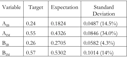
Unfortunately, the decision maker has been unable to gather the necessary values to populate the expert judgment variables on the expected growth between each system. Using the above observations, Table 3 displays the output of the model. In brackets is the percentage the standard deviation dropped by using the observations.
Variable Target Expectation Standard
Deviation
AIB 0.24 0.1824 0.0487 (14.5%)
AIM 0.55 0.4326 0.0846 (34.0%)
BBIB 0.26 0.2705 0.0582 (4.3%)
BBIM 0.57 0.5302 0.1014 (14%)
Table 3 – Adjusted beliefs given observations
8. Sensitivity Analysis
If similar modeling had been carried out using a probabilistic approach, it is unlikely that sensitivity analysis could be carried out. Due to the simplicity of the Bayes linear formulas, sensitivity analysis can be carried out quickly. Three scenarios can potentially be investigated; we could modify our prior belief about our expectations, modify our prior beliefs regarding the covariance matrix, or consider potential sources of observations that have yet to be collected. The purpose of the sensitivity analysis is to analyze whether or not different scenarios would have had an effect on whether or not we believe the systems have met reliability requirements.
8.1 Adjusting Prior Expectations
Given the current covariance matrix and observations, we assess how much the decision maker's prior belief in E(AIB), E(AIM), E(BIB), and E(BIM), would have to increase by in order that his adjusted expectation is greater than the targets. In order to do this, we assume the covariance structure between the observed values and the value of interest remains the same.
[image:10.595.91.352.284.401.2]than the target. If the prior expectation of BIB was lowered from 0.302 to 0.2548, the adjusted expectation of BIB given the observations would be equal to the target of 0.26. If the prior expectation of BIM was raised from 0.578 to 0.7799, the adjusted expectation of BBIM given the observations would meet the target of 0.57. The decision maker stated for
the three reliability requirements that the contractor is currently not meeting; the proposed prior beliefs do not present his `true' belief about the reliability of the vehicles.
8.2 Adjusting Covariance Matrix
The aim of adjusting the covariance matrix is to assess whether or not the observations are having too strong an effect on the decision maker's prior beliefs. Sensitivity analysis is carried out on the residual uncertainty between the true reliability value and the reliability value observed during each phase of the RGT. All the observations made to date have been smaller than their expected value. As three out of the four reliability requirements are not currently being met, decreasing the residual variance, i.e. increasing the correlation between the observation and the `true' reliability of the system, will make the adjusted expectation of the requirements decrease further. By lowering the correlation between the observations and `true' reliability, more faith is placed in the prior belief of the decision maker and the adjusted expectation of the parameters of interest will rise.
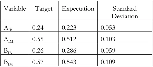
At this time, the decision maker believes the observed basic reliability value will fall between -0.05 and 0.05 of the ‘true’ value. The decision maker believes the observed mission reliability value will fall between -0.1 and 0.1 of the `true' value. Two scenarios will be investigated. The first scenario is increasing the basic reliability range to -0.1 and 0.1 and the mission reliability to -0.2 and 0.2. The second scenario is increasing the basic reliability range to -0.15 and 0.15 and increasing the mission reliability range to -0.3 and 0.3. These two scenarios have the effect of changing the residual variance between the ‘true’ reliability and observed reliability and essentially reducing the strength of the relationship between the observed value and the ‘true’ reliability. The result of each scenario can be found in Table 4 and Table 5.
Variable Target Expectation Standard
Deviation
AIB 0.24 0.223 0.053
AIM 0.55 0.512 0.103
BBIB 0.26 0.286 0.059
[image:11.595.89.353.489.606.2]BBIM 0.57 0.543 0.109
Table 4 – Adjusted beliefs given observations for Scenario 1
Variable Target Expectation Standard
Deviation
AIB 0.24 0.268 0.055
AIM 0.55 0.548 0.114
BBIB 0.26 0.291 0.06
BBIM 0.57 0.553 0.113
Table 5 – Adjusted beliefs given observations for Scenario 2
It can be observed from the tables above that changing the residual uncertainty of the observations does not strongly affect the adjusted beliefs of Vehicle B. The largest impact of changing the residual uncertainty of the observations occurs for Vehicle A's basic and mission reliability. In Scenario 2 where the correlation is substantially reduced, the adjusted expectation for the basic reliability is greater that the target and the adjusted expectation for the mission reliability are only slightly below the target. However, the decision maker did not believe that it was realistic to think the residual uncertainty could potentially as high as in Scenario 1 or 2.
8.3 Potential Sources of Observations
The third form of sensitivity analysis is to consider the observations that have yet to be received. In this case, it may still be possible to gather the expert's opinion on the growth between the basic and mission reliability of each vehicle after the third phase of RGT's and prior to the vehicle entering service. We are interested in knowing what values for EGA3,IB EGA3,IM and EGB3,IM will result in the respective vehicle meeting their respective requirement. EGB3,IB is ignored as it is already on target to meet requirements. In order for the vehicles to meet reliability requirements, the expert must state three values; EGA3,IB = 0.075, EGA3,IM = 0.28, and EGA3,IM =
0.0585. Each of these three values is outside the range of values the decision maker specified that he thought the expert may state.
9. Summary of Analysis
Based on the prior belief stated by the decision maker and the observations made, the contractor, at this stage, has not given the decision maker sufficient evidence to suggest they are meeting all four reliability requirements. The model indicates the expectation of Vehicle B's basic reliability is greater than the target. However, the expectation of both of Vehicle A's reliability requirements and Vehicle B's mission requirement is lower than the target. In the case of Vehicle A, the probability of meeting the target is small.
Extensive sensitivity analysis has been carried out to investigate whether or not the three reliability requirements currently not being met could be met given changes in the prior specification by the decision maker. Two scenarios of particular interest were investigated; first, what changes could be made to the prior expectation so that requirements are being met, and second, what changes could be made to the covariance structure in order that reliability requirements were met. For the three reliability requirements currently not met, the decision maker did not believe it was feasible to modify his prior belief structure to such an extent that the adjusted expectation of each of the three requirements was greater than the target.
10. Acknowledgements
11. References
1. Goldstein, Michael. "Exchangeable Belief Structures." Journal of the American Statistical Association 81, no. 396 (1986): 971-76.
2. Goldstein, Michael, and David Wooff. Bayes Linear Statistics: Theory and Methods. Chichester, UK: John Wiley & Sons, 2007.
3. Goldstein, Michael, and Tim Bedford. "The Bayes Linear Approach to Inference and Decision-Making for a Reliability Programme." Reliability Engineering and System Safety 92, no. 10 (2006): 1344-52.
4. Craig, P.S., Michael Goldstein, A.H. Seheult, and J.A. Smith. "Bayes Linear Strategies for Matching Hydrocarbon Reservoir History." In Bayesian Statistics 5, edited by J.M. Bernardo, J.O. Berger, A.P. Dawid and A.F.M. Smith, 69-95: Oxford University Press, 1996.
5. Farrow, Malcolm. "Practical Building of Subjective Covariance Structure for Large Complicated Systems." The Statistician 52, no. 4 (2003): 553-73.
6. O'Hagan, Anthony, E.B. Glennie, and R.E. Beardsall. "Subjective Modeling and Bayes Linear Estimation in the UK Water Industry." Applied Statistician 41, no. 3 (1992): 563-77.
7. De Finetti, Bruno. Theory of Probability: A Critical Introductory Treatment 1990 ed. Vol. I and II: John Wiley & Sons Ltd., 1974.
8. Farrow, Malcolm, Michael Goldstein, and T. Spiropoulos. "Developing a Bayes Linear Decision Support System for a Brewery." In The Practice of Bayesian Analysis, edited by Simon French and J.Q. Smith: Edward Arnold, 1997.
9. Garthwaite, Paul H., and Anthony O'Hagan. "Quantifying Expert Opinion in the UK Water Industry: An Experimental Study." The Statistician 49, no. 4 (2000): 455-77. 10. Kadane, Joseph B., and Lara J. Wolfson. "Experiences in Elicitation." The Statistician
47, no. 1 (1998): 3-19.
11. Revie, Matthew (2007) Evaluation of Bayes Linear Modelling to Support Reliability Assessment During Procurement. PhD Thesis University of Strathclyde
12. Pearson, E.S., and J.W. Tukey. "Approximate Means and Standard Deviations Based on Distances between Percentage Points of Frequency Curves." Biometrika 52, no. 3 and 4 (1965): 533-46.
13. Keefer, Donald L., and Samuel Bodily, E. "Three-Point Approximations for
Continuous Random Variables." Management Science 29, no. 5 (1983): 595-610.
12. Biographies
Tim Bedford, MSc, PhD
Department of Management Science University of Strathclyde
40 George Street, Glasgow, G1 1QE, UK e-mail: [email protected]
Tim Bedford is Professor of Risk Assessment and Decision Analysis at the University of Strathclyde, Scotland. Tim has co-authored the book “Probabilistic Risk Assessment” with Roger Cooke and has published many papers in risk and reliability analysis.
Richard Denning, MSc
United Kingdom Ministry of Defence
Ash #3308, Abbey Wood, Bristol, BS32 8JH, UK e-mail: [email protected]
Richard Denning is the President of the UK Safety and Reliability Society and Head of Reliability Policy within the UK Ministry of Defence.
Matthew Revie, MSc
Department of Management Science University of Strathclyde
40 George Street, Glasgow, G1 1QE, UK e-mail: [email protected]
Matthew Revie is a researcher at the University of Strathclyde, Scotland, working with the UK Ministry of Defence on Bayes Linear modelling. Matthew is in the process of completing his PhD and is the corresponding author for this paper.
Lesley Walls, PhD, CStat
Department of Management Science University of Strathclyde
40 George Street, Glasgow, G1 1QE, UK e-mail: [email protected]