Copulas for statistical signal processing (part II) : simulation, optimal selection and practical applications



1

Centre for excellence in Signal and Image Processing (CeSIP), Dept. of Electronic and Electrical Engineering, University of Strathclyde, Glasgow, United Kingdom 2

School of Computer Science and Technology, Tianjin University, Tianjin, China

Abstract—This paper presents algorithms for generating random variables for exponential/Rayleigh/Weibull, Nakagami-m and Rician

copulas with any desired copula parameter(s), using the direct conditional cumulative distribution function method and the complex

Gaussian distribution method. Moreover, a novel method for optimal copula selection is also proposed, based on the criterion that for a

given series of copulas, the optimal copula will have its copula density based mutual information closest to the corresponding bivariate

distribution based mutual information. The corresponding bivariate distribution is the bivariate distribution that is used to derive this

copula. Akaike information criterion (AIC) and Bayes’ information criterion (BIC) are compared with the proposed mutual information

based criterion for optimal copula selection. In addition, several case studies are also presented to further validate the effectiveness of the

copulas, which include dual branch selection combining diversity using Nakagami-m, exponential/Rayleigh/Weibull and Rician copulas

with different marginal distributions as in real applications.

Index Terms—Copulas, statistical signal processing, copula random variables generation, optimal copula selection

*Corresponding Author: Dr. J. Ren,

Centre for excellence in Signal and Image Processing Dept. of Electronic and Electrical Engineering# University of Strathclyde,

204 George Street, Glasgow, United Kingdom

Email: [email protected]

Phone: +44-141-5482384

Copulas for Statistical Signal Processing (Part

II): Simulation, Optimal Selection and

Practical Applications

1. INTRODUCTION

One of the most important advantages of copulas is to generate correlated random variables with arbitrary marginal distributions. However, obviously, this requires the successful generation of random variables for copulas. Copula random variables generation is also called copula simulation, which is widely used for constructing corresponding statistical models [1]. Once a suitable copula (an optimal copula) that can accurately model the dependence between marginal distributions is determined, the marginal variables x

and y can be generated by their inverse marginal cumulative distribution function (cdf), based on the fact that the variables u and v

of copula function are both uniformly distributed [1, Sec. 2.9]. Obviously, to utilize a copula function, generating random variables for the copula function is essential. In Part I of this paper, we have derived the copulas for Nakagami-m, exponential/Rayleigh/Weibull, and Rician distributions. And in this part, we will focus on algorithms for generating random variables for these copulas as no such algorithm have been presented so far.

Note that selecting a suitable copula is quite important for modeling dependence correctly between marginal distributions, and optimal copula is only determined by the marginal distributions. The empirical copula, graphic plot and Akaike information criterion (AIC) are popular methods currently for choosing optimal copula [2], and a good survey regarding this topic can be found in [3]. However, the empirical copula based method is too time consuming, thus it is not suitable for large dataset. The graphic plot based method chooses the optimal copula visually and thus is not suitable for real-time signal processing. Since AIC is a likelihood-based method, usually it requires extremely large dataset for model selection.

In this paper, a novel mutual information based method for automatic selection of optimal copulas is also presented, which suits for the case when the associated copula density functions and their corresponding joint probability density functions (pdf) are available. There are three popular methods for copula parameter estimation. The first method is the Kendall‟s tau or Spearman‟s rho based method [4, Sec. 3.1.2], [4, Sec. 3.1.3], this method requires an analytical expression linking the copula parameter and

Kendall‟s tau or Spearman‟s rho, and such expressions are not available for Weibull/exponential/Rayleigh, Nakagami-m and Rician

copulas. Besides, the maximum likelihood estimation (MLE) is quite popular for copula parameter estimation. Let





T t t

t

X  X X _ denotes a observation sample, where _X1t _and 2 t

X are two vectors with the length T, the expression of

log-likelihood of joint probability density function can be written in terms of the copula density and marginal probability density

functions as [4, Sec. 5.2]:

2 1 1 1 2 2 2

1 1 1

( ) ln ( ( , ), ( , )) ln ( ; )

T T

t t t

n n n

t t n

c F x F x f x

   

  







where c is the copula density function, F1 and F2 are two marginal cumulative distribution functions (cdf) with parameters θ1 and θ2

called Inference for Margins (IFM) which estimates the copula parameter by two steps [4, Sec. 5.3]: Step 1: ) ; ( ln max arg ˆ 1 2 1 n T t n t n n

n f x







 



Step 2: Estimate the parameter(s)



ˆ

) ), ; ( ), ; ( ( ln max arg ) ( max arg

ˆ _{2 2 2}

1

1 1

1













  (2)

The second MLE method is called Canonical Maximum Likelihood method (CML), it estimates the copula parameter(s)



ˆ

follows [4, Sec. 5.4]: the data _x1t _and 2 t

x are first transformed into the uniform variants by using empirical distributions, then use

the following MLE in Eq. (3) to estimate the parameters



ˆ

_{ˆ argmax} 2 _{ln ( , ; )} 1 2 1







c (3)

The empirical distribution is defined as:

1 1 ( ) ( ) n n i i

F x I X x

n 





,

1 ( )

0 A

if x A

I x

if x A

 

  _

 .

The CML method considers the attractive advantage of copula that copula separates the dependence structure and marginal

distributions since the marginal distribution are usually unknown, and it is suitable for all the copulas mentioned in this paper. Thus

we always adopt CML as a universal method for copula parameter estimation in this paper.

The remainder of this paper is organized as follows. Section II discusses methods for generating random variables for exponential/Rayleigh/Weibull, Nakagami-m and Rician copulas using univariate marginal cdf method. In Section III, a novel method for optimal copula selection based on mutual information is proposed. Section IV presents case studies to apply these copulas in applications of dual branch selection combining diversity problems in communication field. Concluding marks are summarized in Section V.

2. COPULA RANDOM VARIABLES GENERATION

Let FX(.) and FY(.) be two marginal cumulative distribution functions (cdf) for random variables x and y, respectively, the

corresponding bivariate copula function is given below [1, Sec. 2.3]:

1 1

( , ) XY( , ) XY( X ( ), Y ( ))

where the simulation task here is to generate uniformly distributed random variables (u, v) whose joint distribution function is C. One of the most commonly used approaches for generating copula random variables is the conditional copula method, and the conditional copula is defined as [1, Sec. 2.9]:

0

( , ) ( , ) ( , )

( ) Pr( | ) lim

u _u

C u u v C u v C u v

c v V v U u

u u



  

    

 (5) where c v_u( )is the partial derivative of the copula, a non-decreasing function which exists for almost all v[0,1].

The conditional copula based method can be described in the following three steps:

1) Generate two independent uniform random variables t₁ andt₂ [0,1];

2) Letut₁,c v_u( )t₂;

3) Compute 1

2 ( ) u

vc t , and the pairs (u, v) are then regarded as the desired copula random variables, where 1 u

c denotes a quasi-inverse of c_u. The definition of the quasi-inverse function can be found in [1, Sec. 2.3].

As can be seen, conditional copula based method is quite intuitive and works well for some copulas, especially for Archimedean copulas where the analytical expression of 1

u

c () is resolvable. However, in more complicated cases, it is extremely difficult to find the analytical expression of 1

u

c (). To this end, an alternative approach using univariate marginal cdf should be applied as discussed below.

For a specific copula, the univariate marginal cdf based method can also be summarised in the following three steps [4, Sec. 6.2]:

1) Generate two independent uniform random variables t₁ andt₂ [0,1];

2) Generate random variables pairs (x, y) from t1 and t2 according to their bivariate distribution;

3) Let uFX( )x andvF yY( ), and the pairs (u, v) are then taken as the desired copula random variables.

Note that F_X()and FY() are the marginal cdfs used to derive the copula. Apparently the univariate marginal cdf based method requires that the random variables pairs (x, y) themselves can be generated before the generation of the copula random variables. In this paper, the univariate marginal cdf based method will be employed for copula random variables generation since it is too difficult to directly derive the analytical expression of 1

u

c (.) for our newly derived copulas.

2.1. Bivariate Exponential/Rayleigh/Weibull Copula

In Part I of the paper [20], we have derived the bivariate exponential (also Rayleigh and Weibull) copula function as:

ds s a I e e ds s a I e e v u C a s a a s a a ) 2 ( ] 1 ) 2 ( [ 1 ) ,

( 0 1

0 1 0 0 2 1 2 2 2







 (6)

where a1ln(1u)/









Alternatively, it can be also defined by using Marcum‟s Q function as [20]:

)) , ( 1 )( 1 ( ) , ( ) 1 ( 1 ) ,

(uv vQ1 u1 v1 u Q1 u1 v1

C         (7)

where 1

1 2ln(1 )( 1)



 

 u



u and 1

1 2ln(1 )( 1)



 

 v



v .

To generate random variables for exponential, Rayleigh and Weibull copulas, we need first generate random variables (x, y) for bivariate exponential/Rayleigh/Weibull distribution before the univariate marginal cdf method can be applied. To this end, two methods, based on inverse cdf and complex Gaussian distribution, respectively, are utilized as discussed below.

2.1.1 Inverse cdf based univariate marginal CDF method

The exponential copula has been proved to be equivalent to the Rayleigh and Weibull copulas, thus we only take exponential copula as an example for random variable generation of these three copulas. Note that same results are achieved if we choose bivariate Rayleigh or Weibull distribution to generate random variables for the three copulas.

Firstly, we generate two independent uniform random variables t₁ andt₂[0,1]. And then we compute the conditional pdf of

y given x for bivariate exponential distributions by:

| 0

( , ) 2

( | ) exp( ) ( )

( ) 1 1 1

XY Y X

X

f x y x y

f y x x I xy

f x

 _   _

  



  

   (8)

The associated conditional cdf can be derived as:

| 0

0

2

( | ) exp( ) ( )

1 1 1

y Y X

x s

F y x    I xs ds

  



 

  



Note that the Marcum Q function is defined as

2 2 1 2 1 ( , ) ( ) ( ) x a m m m b x

Q a b x e I ax dx

a

 _  





_

Marcum‟s Q function becomes

2 2

2

1( , ) 0( )

x a

b

Q a b xe I ax dx  _ 



_

2 2 1

1 0

( , ) 1 exp( ) ( )

2 b

m m

m m

a x

and again for the special case with m = 1, we have

2 2

1 0

0

1 ( , ) exp( ) ( )

2

b

a t

Q a b t  I at dt

 

_

derive

| 1

2 2

( | ) 1 ( , )

1 1

Y X

x y

F y x  Q _ _

  . LetFY X| ( | )y x t2, we can also derive that

1

1 2

1 2

( ,1 )

2 1

x y _Q _ t

 , Note that if Q a b1( , )s,

we have 1 1 ( , )

Q a s b, where 1 1 ( , )

Q a s denotes the inverse Marcum Q function on variable b. Let 1

1 1

1

( ) ln(1 )

X

x F t t

 

    , as a

result, (x, y) are desired random pairs for bivariate exponential distribution. Note that the pairs (x, y) depends on three parameters, ,

 and. Finally, we have 1 1 2

1 2

2 ln(1 ) 1

( ) 1 exp( ) 1 exp{ [ ( ,1 )] }

2 1

Y

t

vF y   y     Q   _ t

 .

Let u = t1, then the pairs (u, v) are the desired random variables for bivariate exponential, Rayleigh and Weibull copulas. It can be

found that the correlated exponential distributed pairs (x, y) depends on the parameters , and, while the random variables of bivariate exponential, Rayleigh and Weibull copulas are only depends on the parameter . This can be also validated by Eq. (6) or Eq. (7). In other words, this means that copulas have helped to simplify the dependence structure of these random variables whilst preserving the most significant characteristics among them.

2.1.2 Complex Gaussian distribution based univariate marginal CDF method

Since multivariate Rayleigh distribution can be represented using a set of zero-mean complex Gaussian random variables as

0 0

( 1 ) ( 1 )

k k k k k

G  X  X i Y  Y , where k = 0,1,2…L, i 1 and X Y_k, _k G(0,1/ 2) are independent [5], complex Gaussian random variables can be used to generate random variables for Rayleigh copula as well as its equivalences, i.e. exponential and Weibull copulas.. Here, we haveGK CG(0,1/ 2), where G( ) and CG( ) represent Gaussian distribution and complex Gaussian distribution, respectively. As a result, |GK|is a set of Rayleigh random variables, and we can derive the mean-squared value of |G_k| is _{(| | )}2 2

k k

E G  . Note that _{(| | )}2

k k

E G   , thus we have

0 0

( 1 ) ( 1 )

k k k k k

G   X  X  i Y  Y (11)

where ρ refers to the cross-correlation coefficient between any Gk and Gj (k≠j).

Let 2 2

1 1 1 0 1 0

| | ( 1 ) ( 1 )

xG   X  X  Y  Y and 2 2

2 2 2 0 2 0

| | ( 1 ) ( 1 )

yG   X  X  Y  Y , as a result, (x, y) are desired random pairs for bivariate Rayleigh distribution. Consequently, we can simulate (u, v) for exponential/Rayleigh/Weibull copulas by computing:

2 2

1 0 1 0

1 exp{ [( 1 ) ( 1 ) ]}

2 2

2 0 2 0

1 exp{ [( 1 ) ( 1 ) ]}

v   X  X  Y  Y

Note that the generation of correlated Rayleigh distributed pairs (x, y) depends on the parameters  _X, _Y and . However, the generation of random variables for bivariate exponential/Rayleigh/Weibull copulas only depends on the parameter .

2.2. Bivariate Nakagami-m Copula

Similar to the bivariate exponential/Rayleigh/Weibull copulas, both inverse cdf based method and complex Gaussian distribution based method are utilized to generate random variables (u, v) for bivariate Nakagami-m copula as presented below.

2.2.1 Inverse cdf based univariate marginal CDF method

The Nakagami-m copula has been defined as [6]

1 1

0

(1 ) ( ) ( , ) ( , )

( , ) [ ] [ , ] [ , ]

( ) 2 ! 1 1

m k

k

m k P m u P m v

C u v P m k P m k

m k

 

 

 





  

  





To simulate random variables for Nakagami-m copula, we firstly generate two independent uniform random variables t₁

andt₂[0,1]. According to the definition of bivariate Nakagami-m pdf and marginal Nakagami-m pdf in [20, Sec. 2.4], we can derive the conditional pdf of y given x for bivariate Nakagami-m distributions as:

1 ( 1)/2 2 2

| ( 1)/2 ( 1)/2 1

2

2 ( / / )

( | ) exp( ) ( )

(1 ) 1 1

m m m

X X Y

Y X m m m

Y X Y

mxy

mx y m x y

f y x  I 

   

 

  

   

 

      (13)

The associated conditional cdf can be derived as by applying Eq. (10):

|

2 2

( | ) 1 ( , )

(1 ) (1 )

Y X m

X Y

m m

F y x Q x  y

 

 

    (14)

LetF_{Y x|} ( | )y x t₂, thus we have 1

2

(1 ) 2

[ ,1 ]

2 (1 )

Y m

X m

y Q x t

m

 

 

 

 

  , where m is positive integer. However, in some applications,

the parameter m of the Nakagami distributions can be non-integer. For these cases, we can consider that the generalized Marcum Q

function is the complementary cdf of the noncentral chi-squared distribution with 2m degrees of freedom, where 2m is not

necessarily an integer [18]. The relationship between generalized Marcum Q function and noncentral chi-squared distribution can

be expressed as _{1 ( , ) (} 2_{,2 ,} 2₎ m

Q a b K b m a

  , where K() denotes the non-central chi-squared distribution, and λ is called

noncentrality parameter. Let Q a b_m( , )y, we can derive that the inverse Marcum Q function about its second variable as

1 1 2

( , ) (1 ,2 , )

m

Let 1 1

1 1

( ) X ( , )

X

x F t P m t

m

  

   , then (x, y) are the desired random pairs for bivariate Nakagami-m distribution. Note that Eq.

(14) is different from Eq. (5) in [7] since the Nakagami-m distribution in this paper is defined as _{( )} 2 2 1_exp( 2₎

( )

m m

X m

X X

m x mx f x

m



 

   , where

it is defined in a different way as _{( )} 2 2 1 _exp( 2 ₎

( ) m X m X X x x f x m   

   in [7]. However, the same expression of Nakagami-m copula can be

derived from these two different definitions. As a result, we have 2 1 1 1 2

2

2 ( , )

1

( ) ( , ) ( , [ ( ,1 )] )

2 1

Y m

Y

P m t my

v F y P m P m  Q  t

          .

Finally, let u = t1 , the pair (u,v) becomes the desired random variables for bivariate Nakagami-m copula. As can be seen, the

generation of random variables only depends on the parameters  and m, just as validated in Eq. (12).

2.2.2 Complex Gaussian distribution based univariate marginal CDF method

Complex Gaussian random variables can also be used to generate random variables for Nakagami-m copula as multivariate Nakagami-m distribution can be represented by using a set of zero-mean complex Gaussian random variables defined in [5] as

0 0

( 1 ) ( 1 )

kj k kj j k kj j

G  X  X i Y  Y

where k=0,1,2…L; j=1,2…,m; i 1, and X_kj,Y_kj G(0,1/ 2) are independent to each other. Consequently, we have (0,1/ 2)

kj

G CG , where again G( ) and CG( ) represent Gaussian distribution and complex Gaussian distribution, respectively. The

cross-correlation coefficient between any Gkj and Gln (k≠ j and j = n) is denoted as ρ. We can easily derive that 2 1 | | m k kj j N G 





of Nakagami-m random variables, and the mean-squared value of Nk is 2

2 ( k )

k N

E m

m   . Note that the mean-squared value also equals_k. Consequently, we have

0 0

( 1 ) ( 1 )

k k

kj kj j kj j

G X X i Y Y

m   m  

 

      (15)

Let 2 1 2 2

1 1 0 1 0

1 1

| | [( 1 ) ( 1 )

m m

j j j j j

j j

x G X X Y Y

m    

 









2 2 0 2 0

1 1

| | [( 1 ) ( 1 )

m m

j j j j j

j j

y G X X Y Y

m    

 









y) are taken as the desired random pairs for bivariate Nakagami-m distribution. As a result, (u, v) are determined by

2 2

1 0 1 0

1

( , [( 1 ) ( 1 ) ])

m

j j j j

j

u P m X X Y Y







2 2

2 0 2 0

1

( , [( 1 ) ( 1 ) ])

m

j j j j

j

v P m X X Y Y



It can be found again that the Nakagami-m copula random variables only depend on the parametersand m.

2.3. Bivariate Rician Copula

The bivariate Rician copula has been derived in Part I of the paper [20] as:

2 1 2 1 2 2 1 0 0 0 2 2 2 2 2 1 2 2 1 ₎ 1 ( ) 1 ( ) 1 ( ) ) 1 ( 2 ) 1 ( 2 exp( 1 ) , ( 1 2 dz dz z z I z z I z z I z z z z z v u

C k k

k k k b b                  

_{ }



where 1

1 1 ( ,1 )

b Q z u and 1

2 1 ( ,1 )

b Q z v .

Alternatively, it can be also defined by using infinite series representation as [20]:

) ) 1 ( 2 )] 1 , ( [ , 1 ( ) ) 1 ( 2 )] 1 , ( [ , 1 ( )! ( )! ( )! ( ! ! ! 2 ) 1 ( ) 1 ( ) 1 ( ) 1 exp( ) , ( ₂ 2 1 1 2 2 1 1 0 , , ' ' 2 2 ' 1 ' 1 0 2                                     





k m n u z Q k m l k n k m k l n m l z z v u C n m l l l k m l l k k

k (17)

For bivariate Rician distribution, it is difficult to find the analytical expression for conditional cdf of y given x. However, complex Gaussian distribution based method can still be applied for Rician copula random variables generation as the multivariate Rician distribution can be represented by a set of non-zero means complex Gaussian random variables given in [4] as

0 0

( 1 ) ( 1 )

k k k

G  X  X i Y  Y (18)

In Eq. (18), (0, )1 2

k

X G and (0, )1

2

k

Y G are independent to each other, where k= 1,2,…,L; ₀ ( ₁, )1 2

X G m and ₀ ( ₂, )1 2

Y G m are also

independent; m1 and m2 can be arbitrary but satisfying 2 2

1 2

m m a. Here, we can simply let _{1 2} 2

2

a

m m  , thus we

have ( ( 2 2 ), )

2 2

K

a a

G CG  i  , where G( ) and CG( ) represent Gaussian distribution and complex Gaussian distribution,

respectively. As a result, |Gk| is a set of Rician random variables. Again the cross-coefficient between Gk and Gj (k≠j) is denoted as ρ, and the mean-squared value of |Gk| is derived as E G(| k| )2 2(1a2). Note that the mean-squared value of |Gk| equals to

2 2

2

a   . Letz a 

 , we can derive 2 2 2

2 2 1 1 a z a z      

 , where

2 1

a 

 .

As a result, we have

2 2

1 1 0 1 0

| | ( 1 ) ( 1 )

xG  X  X  Y  Y

2 2

2 2 0 2 0

| | ( 1 ) ( 1 )

where 2

0

1 1

( , )

2 2

z X G



 _and 2

0

1 1

( , )

2 2

z Y G



 _{, and (x, y) are desired Rician random pairs. Consequently, bivariate Rician copula}

random variables (u,v) can be obtained as

2 2

1 1 0 1 0

1 ( , ( 1 ) ( 1 ) )

u Q z X  X  Y  Y

2 2

1 2 0 2 0

1 ( , ( 1 ) ( 1 ) )

v Q z X  X  Y  Y

Please note the generation of Rician random pairs (x, y) depends on three parameters, i.e.



,

z



,

a

2.4. Comparison of the inverse cdf based method and complex Gaussian based generation of copula random variables

The inverse cdf based method for generating random copula variables is an intuitive method, and it suits for the

Weibull/exponential/Rayleigh and Nakagami-m copula with non-integer m, while integer m is required for complex Gaussian based

method. However, the inverse cdf based method usually needs to find an analytical expression of conditional pdf of bivariate

distribution, which may be very difficult to achieve. For example, the inverse cdf based method is not applied for the Rician copula,

as an analytical expression of conditional associated pdf cannot be derived. In addition, the inverse cdf based method is required to

calculate the inverse Marcum Q function, and this increases the computational cost. The complex Gaussian distribution based

method can be applied for the Weibull/exponential/Rayleigh and Rician copulas. However, it is only valid for Nakagami-m copula

when the integer m is positive.

3. OPTIMAL COPULA SELECTION

For a given problem, optimal copula selection is always important for practical applications in accurately modeling of the data. Currently, empirical copula [1, Sec. 5.6], [8], graphic plot [9], AIC [3], [10] and [11] are three most popular used methods for optimal copula selection, and a good survey regarding this topic can be found in [3].

Let {( , )}n ₁ k k k

x y _ denotes a sample of size n from a continuous bi-variate distribution, and the empirical copula C_n can be defined as [1]:

( ) ( ) (number of pairs(x, y) in the sample with , )

( , ) i i

n

x x y y

i j

C

n n n

 

where xx_{( )}i,yy_{( )}i,1i j, n denotes order statistics from the sample. The candidate of copula is thought as the optimal copula

if it has the minimal Euclidean distance with the empirical copula. However, the empirical copula based method is usually time consuming, thus it is not suitable for large dataset and real-time processing. Graphic plot based method selects the optimal copula by visually inspecting the scatter plots of the observation data and simulated results, and therefore it is not suitable for real-time processing as well.

AIC [3][11] is defined as

1 2

2log[ ( ,_k ) | ] _k

AIC  c u u  q (20) where k is the copula function index; qk2pkand pkisthe number of parameter of the k

th _copula;c

k is the likelihood function

corresponding to the kth copula evaluated by substituting the CML of Eq. (3) as MLE. Note that using empirical distribution u1 and

u2 has been transformed to uniform distribution from observations 1 t

X and _X2t_{, respectively. We may also use IFM in Eq. (2) as}

MLE for AIC, though it suffers from unknown marginal distributions. To this end, CML takes into consideration one of the

significant advantage of copula that copula separates the dependence structure and marginal distributions. Another solution is

Bayes‟ information criterion (BIC) with qk pklog( )T , where T is the number of observations [11]. The copula function with the

lowest AIC or BIC is then regarded as the optimal one [3], [11]. It has been pointed out that none of these methods has been proven to be superior in the survey regarding this topic [3]. Therefore, in this paper, a novel method based on mutual information measurement is presented for optimal copula selection, and the results are compared with AIC and BIC.

Mutual information has been employed for measuring the dependence between two marginal distributions in a wide range of applications such as image registration [12], data fusion [13] and MIMO system [14]. Basically, for two random variables X and Y, the mutual information between them is defined as [15]:

,

( , )

( , ) ( , ) log

( ) ( ) XY XY

X Y

X Y

f x y

MI X Y f x y dxdy

f x f y



_

where fXY(x,y) is the joint pdf and fX(x) and fY(y) are the corresponding marginal pdfs for X and Y, respectively. As an special

example, the mutual information for two Gaussian distributions with a correlation coefficient  has a very simple form as [15]:

2 1

ln(1 ) 2

Gau

MI    (22)

Actually, mutual information can also be defined by using a copula density only as [16]:

2

[0,1]

( , ) ( , ) log ( , )

where the copula in Eq. (23) should be a valid copula.

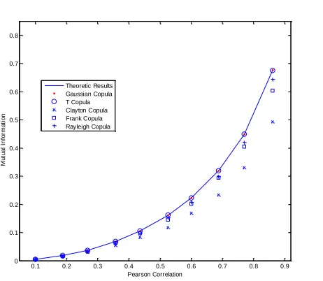
Next we will examine the effect of mutual information for optimal copula selection. Firstly, we generate a series of bivariate Gaussian distribution dataset with size 10000x2 with 10 different Pearson correlations varying from 0 to 1, where the mean values are 5 and 6, respectively and both standard deviations are 1. And then we calculate the mutual information for the bivariate Gaussian distribution using Eq. (22) as the theoretic results. Next, we compute the Clayton, Frank, Gaussian, Rayleigh and Student‟s t copula based mutual information as several candidates, where the density functions for the Clayton, Frank and Student‟s t copulas are given in Table 1 [3]. These copulas density based mutual information, as shown in Figure 1, are computed by the numerical integrals [17] since it is extremely difficult to find their analytical expressions.

From Fig. 1, we can easily make the following observations: i) Both Gaussian copula and Student‟s t copula have generated exactly the same mutual information as expected from the theoretic model, thus either Gaussian or Student‟s t copula can be selected as the optimal copula for these datasets. Note that Student‟s t copula with a large degrees of freedom can be considered as Gaussian copula [3], and this explains the results above; ii) The unsuitable copulas will cause more or less errors to the due dependence, where Clayton copula yields the worse results of the maximum errors.

In addition, to further validate these observations, the simulated datasets (x, y) are obtained by transforming (u, v) according to the Gaussian marginal cdf for these four copulas as shown in Fig. 2. Here, we choose the case of ρ = 0.6, the same results can be obtained as above, it is clear that the Gaussian and Student‟s t copula outperforms Clayton, Frank and Rayleigh copulas for simulating Gaussian distributed datasets as the simulated result has a good matching to the original dataset.

Given a series of copula candidates, the criterion for optimal copula selection based on mutual information is described as follows. First of all, we estimate mutual information from each copula density and also the corresponding bivariate distribution, respectively. Note that the corresponding bivariate of a copula should be the bivariate distribution that is used to derive the copula. Then, we compare how close the two measurements of mutual information are. Eventually, the copula whose copula density based mutual information is closest to its corresponding bivariate distribution based mutual information is determined as the optimal one to be selected.

For example, the bivariate Gaussian distribution is used to derive the Gaussian copula, and thus the Gaussian copula is able to

accurately model the dependence between Gaussian distributed dataset. As a result, for Gaussian distributed dataset, if we examine

the optimal copula between Gaussian and Rayleigh copula, the difference between the Gaussian copula based mutual information

and bivariate Gaussian distribution based mutual information should be smaller than the difference between Rayleigh copula based

mutual information and bivariate Rayleigh distribution based mutual information. This difference can be simply expressed by the

As for the computation of mutual information, an example using Rayleigh copula is presented below. For a given dataset, we need

determine the Rayleigh copula based mutual information and bivariate Rayleigh distribution based mutual information to calculate

their difference. We firstly estimate Rayleigh copula parameter_C, and use it to compute the copula based mutual information.

Next, the parameters (_XY, ΩX and ΩY) for bivariate Rayleigh distribution are estimated and used to decide the bivariate Rayleigh

distribution based mutual information. All the copula density based mutual information, and most bivariate distribution based

mutual information can be computed using numerical integrals [17]. This is simply because there are no analytical expressions for

easily calculating them, except the bivariate Gaussian distribution based mutual information as it can be determined using Eq. (22).

It is worth noting that the proposed method for optimal copula selection does not require any theoretic results, as they are usually unavailable in practical applications due to the fact that their marginal distribution may belongs to the different distribution families. For a series of copula candidates, only the bivariate distributions that are used to derive these copulas are required.This criterion can be validated by the following experiment. We will first generate a series of correlated Rayleigh distributed datasets with size 30000x2 , and parameters    X Y 2under different power correlations varying from 0 to 1, and then we are going to determine that Rayleigh copula is the optimal copula to validate our criterion introduced above.

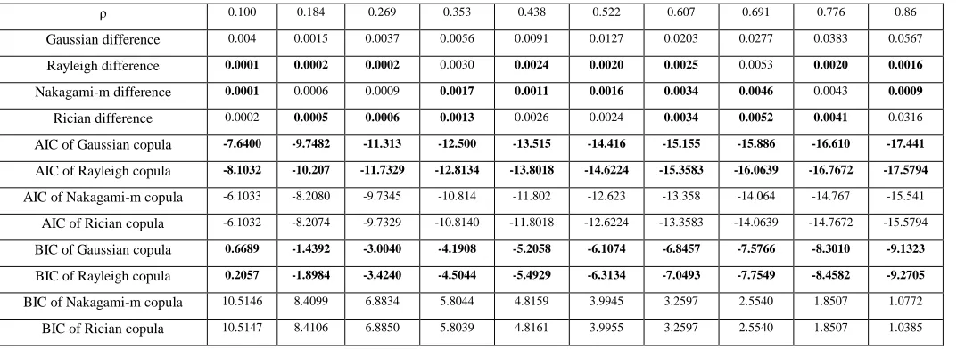
The computed results of optimal copula selection are shown in Table 2. From Table 2, we can find the AIC and BIC based

methods consider correctly Rayleigh copula is the optimal copula, however, they also consider Gaussian copula is „better‟ than

Nakagami-m and Rician copulas for all the 10 bivariate Rayleigh distributed dataset with different power correlation ρ. As a

contrast, the proposed mutual information based method provides more reasonable results, since it considers the Rayleigh,

Nakagami-m and Rician copula are „better‟ than Gaussian copula for all the 10 bivariate Rayleigh distributed dataset with different

power correlation ρ. Note that Rayleigh copula can be considered as a special case of Nakagami-m copula with m = 1, and also a

special case of Rician copula with z = 0, and therefore Rayleigh, Nakagami-m and Rician copulas should be „better‟ than Gaussian

copula for the Rayleigh distributed datasets. We should also note that optimal copula selection is important but difficult due to the

actual data generation mechanism is usually unknown for a given dataset. It is possible that several candidate copulas fit the dataset

well or that none of the candidate of copula fit the data well.

4. CASE STUDIES AND PRACTICAL APPLICATIONS

( ) _XY( , )

F w F w w (24)

In the following, we will generate some correlated random variables by using exponential/Rayleigh/Weibull, Nakagami-m and Rician copulas and their corresponding marginal distributions, and then compute their outage probability for selection diversity systems. Note that in the practical cases, the marginal distribution may be arbitrary, thus the optimal copula must be determined before it is applied for the following on analysis tasks.

4.1 Simulation

Basically, Rayleigh copula-alike random variables means the marginal distributions can be correctly modelled by Rayleigh

copula, where for Nakagami-m copula-alike and Rician copula-alike random variables, the data simulated can be more accurately

modelled using the corresponding Nakagami-m and Rician copulas, respectively. For simulation, we firstly generate 105pairs of

corresponding copula variables ( , )u v , where the parameters for Rayleigh, Nakagami-m and Rician copulas are ( =0.6), ( =0.6,

m=2) and (ρ = 0.7, z = 2), respectively. Accordingly, this ensues the dependence between the marginal distributions are Rayleigh

copula-alike, Nakagami-m copula-alike and Rician copula-alike, respectively, though the actual marginal distribution can be

arbitrary. Note that in practical applications, if the copula is found as the optimal one, this dataset will be considered as

corresponding copula-alike dataset.

After generating random variables for each copula, we transform copula variables (u, v) to random variables (x, y) according to all

other different marginal distributions including Rayleigh, Weibull, Nakagami-m and Rician distributions. Let x FX1( )u



 ,

1_{( )} Y

yF v , w = max(x, y), uwF wX( ) and vwF wY( ), where FX() and FY() represent the cdf of x and y, respectively. Then,

the selection diversity outage probability for Rayleigh copula-like datasets are determined by

ds

s

a

I

e

e

ds

s

a

I

e

e

w

w

F

XY

(

,

)

1

[

(

2

)

1

]

(

2

)

0 1 0 0 2 1 2 2 2



_

_

_

_





where 1

1 ln(1 )(1 )



  

 uw



a and 1

2 ln(1 )(1 )



  

 vw



a .

Alternatively it can also be computed by Marcum‟s Q function as:

))

'

,

'

(

1

)(

1

(

)

'

,

'

(

)

1

(

1

)

,

(

w

w

v

Q

u

v

u

Q

u

v

F

















where 1

1 2ln(1 )( 1) '  uw



u and 1

1 2ln(1 )( 1) ' vw



v .

For Nakagami-m copula-like datasets, the selection diversity outage probability is defined as:

1 1

0

( , ) ( , )

(1 ) ( )

( , ) [ ] [ , ] [ , ]

( ) 2 ! 1 1

m k

w w

XY

k

P m u P m v

m k

F w w P m k P m k

m k              

In addition, the selection diversity outage probability for Rician copula-like datasets is determined by 2 1 2 1 2 2 1 0 0 0 2 2 2 2 2 1 2 2 1 ) 1 ( ) 1 ( ) 1 ( ) ) 1 ( 2 ) 1 ( 2 exp( 1 ) , ( 1 2 dz dz z z I z z I z z I z z z z z w w

F k k

k k k b b

XY _{ }

               





where 1( ,1 ) 1

1 Q z uw

b    and 1( ,1 ) 1

2 Q z vw

b    .

Alternatively, this can also be computed by infinite series as:

1 2 1 2

2 1 ' 1 ' 2 2 '

1 1

' 2 2

0 , , 0

[ ( ,1 )] [ ( ,1 )]

(1 ) (1 )

( , ) exp( ) ( 1) ( 1, ) ( 1, )

1 2 ! ! !( )!( )!( )! 2(1 ) 2(1 )

l l m k l k

XY k l

k l m n

Q z u Q z v

z z

F w w l m k n m k

l m n l k m k n k

                              







where l'lnk.

4.2 Results and Discussions

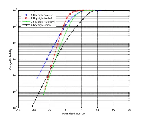
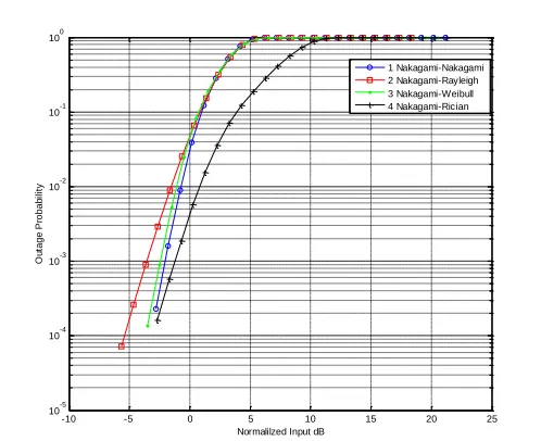
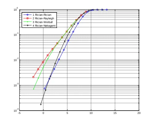
In the case of Rayleigh copula, the first marginal cdf F_X() is always Rayleigh distribution with parameter  2 as shown in Fig. 3. For Nakagmai-m copula case, the first marginal cdf F_X()is always Nakagami-m distribution with parameters  5 and m = 2, and the obtained results are given in Fig. 4. For Rician copula application, the first marginal cdf F_X() is always Rician distribution with parameters  2 and a=4, and the computed results are given in Fig. 5. In other words, these have demonstrated that the optimal copulas have been successfully determined using the proposed approach.

In Figures 3-5, the first marginal distribution is fixed as the Rayleigh distribution, Nakagmai-m distribution and Rician

distribution, respectively, where the second marginal distribution has a set of four values including the Rayleigh, Weibull,

Nakagami-m and Rician distributions. Although  2 is used for the Rayleigh distribution of the second marginal distribution in

all three figures, different parameters are used for other marginal distributions. For Weibull, Nakagami-m and Rician distributions,

the parameters used are ( 2,  5), ( 5,m2) and (a2,  5) in Fig. 3, ( 2, 5), ( 2, m = 3) and (a2, 5

  ) in Fig. 4, and ( 6, 3), ( 6, m = 2) and (a = 2, 2) in Fig. 5, respectively.

To the best of our knowledge, without the copula, the outage probability can be determined only if the marginal distributions

belong to the same family. In other words, take Fig. 3 for example, only Rayleigh-Rayleigh can be obtained, and the results of

Rayleigh-Weibull, Rayleigh-Nakagami-m and Rayleigh-Rician cannot be simulated when copulas are absent. Moreover, the

datasets have a specific dependence structure that can be modelled by using the corresponding Rayleigh copula, and this is why their

marginal distributions that belong to different families of probability distributions cannot be generated without using the Rayleigh

5. CONCLUSIONS

In this paper, three parts of innovative work have been reported in terms of simulation, optimal selection and case studies of copula functions. Firstly, algorithms are proposed for generating random variables for Rician, Nakagami-m, and exponential/Rayleigh/Weibull copulas as no such algorithms exist so far. For all the three groups of copulas, complex Gaussian distribution based method is introduced to generate associated random variables. For the last two groups, how direct conditional cdf method can be applied in generating associated random variables is also given. Secondly, a novel method for selecting the optimal copula by using mutual information is presented. This method has been fully validated by experiments, and is found suitable for all the copulas as long as their copula density functions and their corresponding joint pdfs that are used to derive these copulas are available. Thirdly, case studies are discussed to apply these copulas for outrage probability estimation of selection diversity combining systems in communication based applications. Without using the corresponding copulas, the simulated datasets are required to have the same marginal distributions, yet the copula functions have helped to loosen such constraints in generating arbitrary marginal distributions.

REFERENCES

[1] R. B. Nelsen, An Introduction to Copulas, 2nd ed., New York, Springer Verlag, 2006.

[2] D. Huard, G. Evin, and A. Favre, “Bayesian Copula Selection”, Elsevier Computational Statistics & Data Analysis, Vol. 51, No. 2, pp. 809-822., 2005.

[3] H. Manner, “Modeling Asymmetric and Time-Varying Dependence”, PhD Thesis, Maastricht University, 2010.

[4] U. Cherubini, E. Luciano and W. Vecchiato, Copula Methods in Finance, New York : John Wiley & Sons, 2004.

[5] Y. Chen and C. Tellambura, “Distributions functions of selection combiner output in equally correlated Rayleigh, Rician, and Nakagami-m fading channels”,

IEEE Trans. on Communications, Vol. 52, No. 11, pp. 1948 -1956, 2004.

[6] X. Liu “Copula of bivariate Nakagami-m distribution”, Electronics Letters, Vol.47, No.5, pp.343-345, 2011.

[7] C. Tellambura and A. D. S. Jayalath, “Generation of Rayleigh and Nakagami-m fading envelopes”, IEEE Communications Letters, Vol. 4, No. 5, pp. 170 - 172,

2000.

[8] C. Genest, B. R´emillard, “Tests of Independence and Randomness Based on the Empirical Copula Process”, Test, 13(2), pp. 335-370, 2004.

[9] C. Genest and J. C Boies, “Detecting dependence with Kendall plots,” Amer. Stat., Vol. 57, No. 4, pp. 275–284, 2003.

[10] H. Akaike, “A new look at the statistical model identification, “IEEE Trans. on Automatic Control, Vol. 19, No. 6, pp. 716–723, 1974.

[11] A. Sundaresan and P.K. Varshney, “Location Estimation of a Random Signal Source Based on Correlated Sensor Observations”, IEEE Trans. on Signal

Processing, Vol. 59, No. 2, pp. 787-799, 2011.

[12] J. P. W. Pluim, J. B. A. Maintz, and M. A. Viergever, “Mutual information based registration of medical images: a survey”, IEEE Trans. On Medical Imaging,

Vol. 22, No. 8, pp.986 -1004, 2003.

[13] R. Bramon, I. Boada, A. Bardera, J. Rodriguez, M. Feixas, J. Puig, and M. Sbert, “Multimodal Data Fusion Based on Mutual Information”, IEEE Trans. on

Visualization and Computer Graphics, Vol. 18, No. 9, pp. 1574-1587 , 2012.

[14] A. Goldsmith, S.A Jafar, N. Jindal and S. Vishwanath, “Capacity limits of MIMO channels”, IEEE Journal on Selected Areas in Communications, Vol. 21, No.

[15] C.M Thomas and T.A Joy, Elements of Information Theory, John Wiley & Sons, Inc., 1991.

[16] X. Zeng and T.S Durrani, “Estimation of mutual information using copula density function”, Electronics Letters, Vol. 47, No. 8, pp. 493 - 494, 2011.

[17] W.H. Press, S. A. Teukolsky, W. T. Vetterling, B.P. Flannery, Numerical Recipes in C—The Art of Scientific Computing, 2nd ed., Cambridge, U.K.,

Cambridge Univ. , 1992.

[18] M.K. Simon and M.S Alouini, Digital Communication over Fading Channels, 2nd ed., New York: John Wiley & Sons, 2005.

List of Table/Figure Captions:

Table 1:Density Functions of Clayton, Frank, Gaussian and Student‟s t Copulas Defined in [3], Those for Exponential/Rayleigh/Weibull, Nakagami-m and Rician Copulas Are Given in Part I of The Paper.

Table 2. Computed results of optimal copula selection for Rayleigh distributed dataset

Fig. 1: Mutual information for bivariate Gaussian distribution.

Fig. 2. For Gaussian distributed datasets, simulated results using Gaussian (top-left), Clayton (top-right), Frank (bottom-left) and Rayleigh (bottom-right) copulas.

Fig. 3: Selection diversity combining outage probability for Rayleigh copula-like datasets with different types of marginal distributions.

Fig. 4: Selection diversity combining outage probability for Nakagami-m copula-like datasets with different types of marginal distributions.

TABLEI:DENSITY FUNCTIONS OF CLAYTON,FRANK,GAUSSIAN AND STUDENT‟S TCOPULAS DEFINED IN [3],THOSE FOR EXPONENTIAL/RAYLEIGH/WEIBULL, NAKAGAMI-M AND RICIAN COPULAS ARE GIVEN IN PART I OF THE PAPER

Copulas Copula density functions Parameters

Clayton

1 2 1/

( , ) (1 ) ( 1 )

c u v  



Frank

[ (1 )]( 1 ) (1 ) (1 ) [ ( )] 2

( , )

[

]

u v e

u v u v

e

c u v

e

e

e

e

     











Gaussian _

                ) ( ) ( , 1 1 ) , ( 1 1 ) 1 ( 2 2 2 2 2 2 2 2 2 v v u u e e v u c v u v u v u          

  ( 1,1)

Student’s t

2

1 2 1 2 1 1

2 2

1 1

1 2 1 2

2 2 2 2

[ ( )] [ ( )] 2 ( ) ( )

( 1) ( )(1 )

2 2 (1 )

( , )

1 [ ( )] [ ( )]

1 ( ) (1 ) (1 )

2

v

v v v v

v v

v v

v v t u t v t u t v v

c u v

v t u t v

v v         _    _  _              ( 1,1)  

* Note that In Table 1, Φ() denotes the cdf of standard univariate Gaussian distribution, ()tv denotes the cdf of student T distribution with freedom v,

Table 2. Computed results of optimal copula selection for Rayleigh distributed dataset

ρ 0.100 0.184 0.269 0.353 0.438 0.522 0.607 0.691 0.776 0.86

Gaussian difference 0.004 0.0015 0.0037 0.0056 0.0091 0.0127 0.0203 0.0277 0.0383 0.0567

Rayleigh difference 0.0001 0.0002 0.0002 0.0030 0.0024 0.0020 0.0025 0.0053 0.0020 0.0016

Nakagami-m difference 0.0001 0.0006 0.0009 0.0017 0.0011 0.0016 0.0034 0.0046 0.0043 0.0009

Rician difference 0.0002 0.0005 0.0006 0.0013 0.0026 0.0024 0.0034 0.0052 0.0041 0.0316

AIC of Gaussian copula -7.6400 -9.7482 -11.313 -12.500 -13.515 -14.416 -15.155 -15.886 -16.610 -17.441

AIC of Rayleigh copula -8.1032 -10.207 -11.7329 -12.8134 -13.8018 -14.6224 -15.3583 -16.0639 -16.7672 -17.5794

AIC of Nakagami-m copula -6.1033 -8.2080 -9.7345 -10.814 -11.802 -12.623 -13.358 -14.064 -14.767 -15.541

AIC of Rician copula -6.1032 -8.2074 -9.7329 -10.8140 -11.8018 -12.6224 -13.3583 -14.0639 -14.7672 -15.5794

BIC of Gaussian copula 0.6689 -1.4392 -3.0040 -4.1908 -5.2058 -6.1074 -6.8457 -7.5766 -8.3010 -9.1323

BIC of Rayleigh copula 0.2057 -1.8984 -3.4240 -4.5044 -5.4929 -6.3134 -7.0493 -7.7549 -8.4582 -9.2705

BIC of Nakagami-m copula 10.5146 8.4099 6.8834 5.8044 4.8159 3.9945 3.2597 2.5540 1.8507 1.0772

BIC of Rician copula 10.5147 8.4106 6.8850 5.8039 4.8161 3.9955 3.2597 2.5540 1.8507 1.0385

Note: Gaussian, Rayleigh, Nakagami-m and Rician difference denote the difference between Gaussian copula, Rayleigh, Nakagami-m and Rician copula based

0.1 0.2 0.3 0.4 0.5 0.6 0.7 0.8 0.9 0

0.1 0.2 0.3 0.4 0.5 0.6 0.7 0.8

Pearson Correlation

M

u

tu

a

l

In

fo

rm

a

ti

o

n

Theoretic Results Gaussian Copula T Copula Clayton Copula Frank Copula Rayleigh Copula

0 5 10 0

2 4 6 8 10 12

Gaussian copula

0 5 10

0 2 4 6 8 10 12

Clayton copula

0 5 10

0 2 4 6 8 10 12

Frank copula

0 5 10

0 2 4 6 8 10 12

Rayleigh copula original

simulated

-15 -10 -5 0 5 10 15 20 10-6

10-5 10-4 10-3 10-2 10-1 100

Normalized Input dB

O

u

ta

g

e

P

ro

b

a

b

il

it

y

1 Rayleigh-Rayleigh 2 Rayleigh-W eibull 3 Rayleigh-Nakagami 4 Rayleigh-Rician

-10 -5 0 5 10 15 20 25 10-5

10-4 10-3 10-2 10-1 100

Normalilzed Input dB

O

u

ta

g

e

P

ro

b

a

b

il

it

y

1 Nakagami-Nakagami 2 Nakagami-Rayleigh 3 Nakagami-Weibull 4 Nakagami-Rician

-5 0 5 10 15 20 10-4

10-3 10-2 10-1 100

1 Rician-Rician 2 Rician-Rayleigh 3 Rician-Weibull 4 Rician-Nakagami