LOCAL BIARY PATTERS FOR 1-D SIGAL PROCESSIG
avin Chatlani and John J. Soraghan
Centre for Excellence in Signal and Image Processing (CeSIP), University of Strathclyde Royal College Building, 204 George Street, Glasgow
phone: +(0044) 141 548 2205, email: [email protected], [email protected] http://www.eee.strath.ac.uk
ABSTRACT
Local Binary Patterns (LBP) have been used in 2-D image processing for applications such as texture segmentation and feature detection. In this paper a new 1-dimensional local binary pattern (LBP) signal processing method is pre-sented. Speech systems such as hearing aids require fast and computationally inexpensive signal processing. The practi-cal use of LBP based speech processing is demonstrated on two signal processing problems: - (i) signal segmentation and (ii) voice activity detection (VAD). Both applications use the underlying features extracted from the 1-D LBP. The proposed VAD algorithm demonstrates the simplicity of 1-D LBP processing with low computational complexity. It is also shown that distinct LBP features are obtained to iden-tify the voiced and the unvoiced components of speech sig-nals.
1. ITRODUCTIO
Local Binary Patterns (LBP) have been extensively used in 2-D image processing [1] [2]. LBP has been shown in [3] to be a computationally simple, discriminative descriptor of texture. The motivation for the above applications is that an image can be described by a combination of texture patterns. We aim to develop a 1-D LBP signal processing framework and demonstrate its applicability on a real problem. Real time systems such as hearing aids require fast processing of the input signal while maintaining low computational com-plexity. One common process in speech systems is Voice Activity Detection (VAD) which attempts to estimate peri-ods of speech and non-speech. Different flavours of VAD base their decisions on statistical techniques [4] [8], energy level detection [5] or periodicity measures. VAD perform-ance is affected by the SNR of the noisy speech and per-formance depends on computational complexity and pa-rameter tuning.
In this paper, a novel 1-D LBP operator is developed as a signal processing tool. An LBP code for a neighbourhood of sampled data is produced by thresholding the neighbouring samples against centre samples of a processing window. This procedure is iteratively done across the entire signal and a segment of the 1-D signal is alternatively described by a sparser occurrence histogram of LBP codes. The paper is organized as follows. The novel 1-D LBP operator is pre-sented in section 2. In section 3, a LBP-based segmentation of a 1-D signal is used to illustrate the processing capability of the 1-D LBP. A computationally simple LBP-based VAD
is designed in section 4. This uses the occurrence histogram of the underlying signal to identify the voiced, unvoiced and non-speech components. The performance of the new VAD is demonstrated on a speech sample taken from the TIMIT da-tabase [6] contaminated with non-stationary noise from the NOISEX-92 database [7]. Finally, concluding remarks are presented in section 5.
2. 1-D LOCAL BIARY PATTERS
The 1-D LBP operator is adapted from the 2-D LBP [3]. It examines a neighbourhood of data samples from a signal x[i] and assigns an LBP code to each centre sample after thresh-olding them against the neighbouring samples. The 1-D LBP operating on a sample value x[i] is defined as:
[ ]
( )
[ ]
[
] [ ]
{
}
1 2
2 0
2 1 2
2
P P
P r r
r
LBP x i
P
S x i r x i S x i r x i
−
+
=
= ∑ + − − + + + − (1)
where the Sign function S[.] is given by:
[ ]
10
≥
=
for x 0
S x
for x < 0
(2)
and where the P neighbouring samples are thresholded
around the centre sample from the neighbourhood of P+1
data samples from the signal x[i] of length N for i=[P/2 : -P/2]. The Sign function S[.] transforms the differences to a P-bit binary code. The binomial weight applied to each thresholding operation converts the binary code into a unique LBP code.
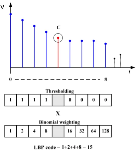
An illustration of the 1-D LBP operator is given in Figure 1 where P is set to 8 and the centre sample C is cir-cled. As in Eq. (1), the 8 neighbouring samples are thresh-olded against C to produce a binary code of 1111_0000. This code is then multiplied by the binomial weights given to the corresponding samples and the obtained values are summed to give the resulting LBP code of 15. The LBP codes can locally describe the data using the difference between a sam-ple and its neighbours. For a constant or slowly varying sig-nal, these differences cluster near zero. At peaks and troughs, the difference will be relatively large, whereas at edges, the differences in some directions will be larger than those from other directions. The local patterns formed from x[i] can be described by the distribution of the LBP codes:
[ ]
( )
(
)
2 2
,
k P
P P
i
H LBP x i k
≤ ≤ −
= ∑ δ (3)
Figure 1 - Computation of 1-D local binary pattern (1-D LBP)
where k=1..n and n is the number of histogram bins and each bin corresponds to an LBP code. δ(i,j) is the Kronecker delta function.
The standard LBPP operator produces 2
P
different LBP
codes. Extensions of the LBPP are presented in [3] for
rota-tion invariant patterns LBPPr, uniform patterns LBPPu, and
rotation invariant uniform patterns LBPPr,u. LBPPr is
pro-duced by shifting the LBP code for the P neighbouring
sam-ples until its minimum value is found. In this way, LBPPr of
the processed window produces the same code for all shifted versions of that code and it is therefore invariant to rotation. A uniform pattern is defined by an LBP code which has at most two one-to-zero or zero-to-one transitions. The remain-ing non-uniform patterns are assigned to a sremain-ingle histogram bin and each uniform pattern is assigned to a separate bin.
LBPPugives a histogram with P(P-1)+3 bins. LBPPr,u shifts
the uniform codes until they attain their minimum values and results in a histogram with P+1 bins for uniform patterns plus one bin for non-uniform patterns. The LBP code evaluated earlier in this section is an example of a code that is uniform and is already rotation-invariant. The choice of which LBP to use depends on the need for either a more resolved represen-tation or for a sparser histogram. In the presented work,
nor-malized histograms will be used for LBPPr,u resulting in
his-tograms with P+2 bins.
3. USUPERVISED SIGAL SEGMETATIO USIG 1-D LBP
The 1-D LBP operator is used to produce a histogram of LBP codes which can be used as an alternative representation of the signal. In signal segmentation, the histogram can be used as a non-parametric estimator of the empirical LBP feature histogram. Resistor Average Difference (RAD) [2] can be
used for measuring the similarity of adjacent LBP histo-grams. RAD is derived from the non-symmetric Kullback-Leibler Distance (KLD) [2] which is used for measuring the difference between two histograms p and q. KLD is given by:
( )
{
(
)
(
)
}
1
( ) lg ( ) lg ( )
n KL
k
D p q p k p k q k
=
=∑ − (4)
where n is the number of histogram bins and p(k) and q(k)
are the number of occurrences in histograms p and q respec-tively at bin k. The RAD is defined as:
(
)
(
( )
)
1(
( )
)
1 1,
RAD KL KL
D p q D p q D q p
−
− −
= +
(5)
DRAD(p,q) between the two histograms p and q increases
with dissimilarity and in contrast to KLD, RAD is symmet-ric [9].
3.1 oise Onset Identification
In this example, the onset of noise is detected for a noise source switched on at some time τ. The signal x is first split
into segments xa[j] of length W by applying a window w[j] of
length W as:
[ ] [
] [ ]
for 0 1a
x j =x aR+j w j ≤ ≤j W− (6)
where a is the segment number, R<W for overlapping
seg-ments and R=W for contiguous segseg-ments. W is chosen to be
small enough to capture transitions in the LBP feature
histo-grams. DRAD(p,q) is measured for the segments of the
adja-cent histograms and similar segments are merged. When two adjacent segments are merged, their histograms are summed and normalized to produce the histogram of the new seg-ment. This procedure continues until the segment does not expand and the previously merged segments are considered as a component of the signal with similar underlying LBP features.
This procedure was performed for an artificially gener-ated sinusoidal signal of length 768 samples which was con-taminated by Additive White Gaussian Noise (AWGN) in the middle portion of the signal as shown in Figure 2(a). The signal was split up as in Eq. (6) with W=128 and R=128 and
a rectangular window w[j]. The 1-D LBP8r,u extension was
used with P=8 to give a LBP histogram with P+2=10 bins as
shown in Figure 2(b) for each segment. The DRAD values for
adjacent segments are shown for illustrative purposes. The results of the segmentation are shown in Figure 2(c) and Figure 2(d). It can be seen that the algorithm exactly sepa-rates the sinusoidal components from the noise affected por-tion based on the similarity of the underlying signal features. No overlap was used in this example, however overlapping the segments will improve fidelity.
4. VOICE ACTIVITY DETECTIO USIG 1-D LBP
Traditional VAD detects speech activity in the presence of noise. VAD does not usually distinguish between voiced and unvoiced components [4][5][8]. Unvoiced speech contains high occurrences of non-uniform patterns and use of the
uni-form LBP extension, LBPPr,u, can distinguish between these
A m p . (a) # o f o cc u rr en ce s # o f o cc u rr en ce s # o f o cc u rr en ce s # o f o cc u rr en ce s # o f o cc u rr en ce s # o f o cc u rr en ce s
Bin # Bin # Bin # Bin # Bin # Bin #
DRAD(p,q)=4x10⁻⁴ DRAD(p,q)=0.0159 DRAD(p,q)=0.0122 DRAD(p,q)=0.0141 DRAD(p,q)= 4x10⁻⁴
(b) A m p li tu d
e 1
-1 Amp
li
tu
d
e 1
-1
[image:3.595.60.541.85.264.2](c) (d)
Figure 2 -Segmentation of a sinusoidal signal contaminated by AWGN (a) Original noisy signal (b) LBP8 r,u
histograms of the 6 seg-ments formed and DRAD(p,q) measure for adjacent histograms (c) Segmented sinusoidal components (d) Noise affected segment
A m p li tu d e (a) # o f o cc u r-re n ce s
Segment number, r
(b) A m p li tu d e (c) # o f o cc u r-re n ce s
Segment number, r
(d)
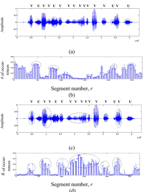
Figure 3 – LBP8r,u results for clean speech utterance (a) Clean
speech with unvoiced segments circled (b) Occurrence results in non-uniform bin 10 from LBP feature histograms (c) Clean speech
with voiced segments circled (d) Occurrence results in central uniform bin 5 from LBP feature histograms
“Good service should be rewarded by big tips” was taken from the TIMIT database [6] and is plotted in Figure 3(a). A sampling frequency of 16 kHz was used and the signal was segmented according to Eq. (6) with a rectangular window of
length W=160 samples and no overlap. The LBP8r,u for each
segment was measured to give LBP histograms with 10 bins. Any non-uniform patterns are separated into a single bin. Figure 3(b) shows the plot for the non-uniform bin (bin 10) for each speech segment. This illustrates that the higher fre-quency unvoiced speech circled in Figure 3(a) and labelled “U” produce higher occurrences of non-uniform patterns. Non-uniform patterns occur in other portions of the signal. This is due to low-power recording noise from the speech sample used. This distinctive non-uniform marker can be used to identify unvoiced speech segments of the analyzed signal that have an increased number of occurrences in the non-uniform histogram bin.
The lower frequency voiced components are highlighted in circles and labelled “V” in Figure 3(c). These produce uniform patterns with the resulting plot shown in Figure 3(d). This shows the number of occurrences in the central uniform bin 5 for the segmented signal. The distribution of the pat-terns for speech signal shows peak activity in the uniform bin 5 at segments corresponding to voiced speech. This LBP feature relates to a particular rotation-invariant feature of the voiced components. It can be seen that during voiced speech activity there is significant activity in this central bin. There-fore, the occurrence histograms of these speech components can distinguish these two regions based on their extracted LBP features. Noise may contain non-uniform patterns and for noisy speech signals, the bin 5 features can also distin-guish unvoiced speech components from weaker voiced speech components that have been more affected by the
added noise. A higher resolved histogram such as LBPPu can
be used if this criterion to distinguish unvoiced speech from noise or weak speech components affected by noise is
re-quired. LBPPu distributes the occurrences in the histogram
over a larger number of bins and thus keeps activity low in any particular uniform bin for unvoiced speech.
Environmental sounds may contain low-frequency noise and periodic components whose spectra overlap with the voiced components of the speech signal. Therefore, discrimi-nation of features that produce similar histograms from
1 2 3 4 5 6 7 8 9 10 1 2 3 4 5 6 7 8 9 10 1 2 3 4 5 6 7 8 9 10 1 2 3 4 5 6 7 8 9 10 1 2 3 4 5 6 7 8 9 10 1 2 3 4 5 6 7 8 9 10 2.5
-2.5 0 100 200 300 400 500 600 700 768
0 100 200 300 400 500 600 700 768 0 100 200 300 400 500 600 700 768
V U V V U V V V V V V V V U V U
[image:3.595.52.286.305.617.2]A
m
p
li
tu
d
e
A
m
p
li
tu
d
e
(a) (a)
A
m
p
li
tu
d
e
A
m
p
li
tu
d
e
(b) (b)
A
m
p
li
tu
d
e
A
m
p
li
tu
d
e
[image:4.595.67.296.81.371.2](c) (c)
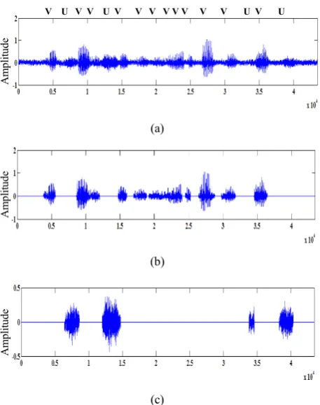
Figure 4 - VAD results for speech contaminated with F16 cockpit noise at 5 dB SNR (a) Noisy speech (b) Voiced speech components
identified (c) Unvoiced speech components identified
Figure 5 - VAD results for speech contaminated with car inte-rior noise at 5 dB SNR (a) Noisy speech (b) Voiced speech components identified (c) Unvoiced speech components
identi-fied
different sound sources is performed by incorporating a local
power measure of the analyzed signal segment xa[j] to give
the joint operator LBPPr,u/VARsegwhere VARseg(xa[j])is given
by:
[ ]
(
)
1[ ]
2 1[ ]
0 0
1 1
( ) where ( )
W W
seg a a a a a
j j
VAR x j x j X X x j
W W
− −
= =
=
∑
− =∑
(7)4.1 1-D LBP-based VAD algorithm
The algorithm presented below uses the 1-D LBP to separate noisy speech into voiced, unvoiced and non-speech compo-nents by the following steps:
1. Segment the input noisy speech signal x to give segments
xa[j]
2. Perform LBP8
riu2
for each segment xa[j] to obtain the
normalized occurrence histogram for that segment
3. Separate all segments which have the normalized
histo-gram bin p(10)>0.3 and label as unvoiced speech
seg-ments. p(k) is the occurrence probability in histogram bin k
4. Measure VARseg(xa[j]) for each segment and separate the
LBP features with VARseg(xa[j])<thresh. Label as
non-voiced speech segments
5. Label remaining segments as voiced speech segments
6. Perform final grouping by assigning contiguous speech
segments TV < 50 ms to non-voiced speech label
The value of thresh must be chosen to distinguish voiced speech from non-speech with similar LBP features. A value of 0.003 for thresh was selected empirically from experimen-tal studies for speech contaminated with different noise types
ranging down to 0dB SNR. The value of TV was chosen as
in [10] to remove the influence of noise intrusion.
4.2 Performance Evaluation
The 1-D LBP-based VAD algorithm from section 4.1 was tested on the previous clean speech utterance from Figure 3(a) degraded with F16 cockpit noise and car interior noise. These noise sources were obtained from the Noisex92 [7] database. Figure 4 shows the results obtained for the speech utterance contaminated with F16 cockpit noise at SNR level of 5 dB with the voiced and unvoiced components labelled “V” and “U” respectively. Figure 4(b) and Figure 4(c) dem-onstrate that the LBP-based VAD algorithm is able to cor-rectly identify all of the voiced and unvoiced components from the noisy speech. Figure 5 shows the results obtained for the speech utterance contaminated with car interior noise at SNR level of 5 dB. Figure 5(b) and Figure 5(c) demon-strate that the LBP-based VAD algorithm is able to correctly identify all of the voiced speech components. However, it does not identify one weak portion of the unvoiced speech since its LBP feature was affected by the stronger low-frequency noise component for low SNR values. The LBP feature for this unvoiced portion was not significantly modi-fied in the previous case with the higher frequency
[image:4.595.319.545.84.371.2]nents of the F16 cockpit noise and therefore resulted in cor-rect identification in that situation.
5. DISCUSSIO
The histogram of the 1-D LBP codes of a signal gives a sparser, alternative signal representation. The LBP operation is fast and computationally inexpensive. It was shown to be a distinctive marker of certain features of the underlying signal. This property has been applied in preliminary work for simple signal segmentation and fast and accurate VAD. The 1-D LBP is able to distinguish the unvoiced and the voiced components of speech signals using the distinguish-ing features of higher activity in certain characteristic histo-gram bins. The use of an overlapping factor will yield im-proved results and give better identification of the onset of distinct signal features. Future work will involve application of the 1-D LBP to signal enhancement and noise estimation techniques. Multi-resolution 1-D LBP will be developed to achieve improved results, especially for analysis of noisy signals. Further work will also involve the inclusion of a joint local variance measure on the samples that produce an LBP code to give improved fidelity.
REFERECES
[1] T. Ojala, M. Pietikäinen, “Unsupervised texture
segmen-tation using feature distributions”, in Pattern Recognition 32, pp. 477-486, 1999.
[2] S. He, J. J. Soraghan et al, “Quantitative Analysis of
Facial Paralysis Using Local Binary Patterns in Biomedical
Videos”, in IEEE Transactions on Biomedical Engineering,
vol. 56(7), pp. 1864-1870, Jul 2009.
[3] T. Ojala, M. Pietikainen, and T. Maenpaa,
“Multiresolu-tion Gray Scale and Rota“Multiresolu-tion Invariant Texture Analysis with
Local Binary Patterns”, in IEEE Transactions on Pattern
Analysis and Machine Intelligence, vol. 24(7), pp. 971-987, 2002.
[4] J. Ramirez, J. C. Segura, J. M. Gorriz, L. Garcia,
“Im-proved voice activity detection using contextual multiple
hypothesis testing for robust speech recognition”, in IEEE
Transactions on Audio, Speech and Language Processing, vol. 15(8), pp. 2177–2189, 2007.
[5] C. Hsieh, T. Feng, P. Huang, “Energy-based VAD with
grey magnitude spectral subtraction”, in Speech Communica-tion, vol. 51, pp. 810-819, 2009.
[6] TIMIT speech database, Speech Enhancement and
As-sessment Resource,
<http://cslu.cse.ogi.edu/nsel/data/SpEAR_noisyspeech.html> [accessed Sep 2009]
[7] NOISEX – 92 Database,
<http://spib.rice.edu/spib/select_noise.html> [accessed Sep 2009]
[8] J. Ramirez, J. C. Segura, C. Benitez, A. de la Torre, A.
Rubio, “Efficient Voice Activity Detection Algorithms using Long-Term Speech Information”, in Speech Communication, vol. 42, pp. 271-287, 2004
[9] D. H. Johnson, S. Sinanovic, “Symmetrizing the
Kull-back–Leibler Distance”, in Technical Report, Rice
Univer-sity, 2001
[10] G. Hu, D. Wang, “Monaural Speech Segregation based
on Pitch Tracking and Amplitude Modulation”, in IEEE