Bayesian decision making for planetary micro-rovers

Bayesian Decision Making for Planetary Micro-Rovers

Mark A. Post

Brendan M. Quine

Regina Lee

York University, 4700 Keele Street, Toronto, Ontario, Canada, M3J 1P3

I.

Introduction

The increasing number of successful robotic systems in place on earth and in space has provided a good precedent for using robots in place of or in concert with humans to perform difficult or dangerous tasks in remote locations. Many technologies are now available for such robots.1 Most of these systems are very complex and specialized, and generally require constant human surveillance to compensate for the limited problem-solving abilities of most robots, requiring large and costly engineering and mission planning teams. It would be beneficial to have a low-cost, self-sufficient robotic system that is capable of overcoming most of the problems encountered in day-to-day operation to accomplish simple mission tasks such as area mapping and object identification. Autonomous planetary vehicles, also commonly known as rovers, are small autonomous vehicles equipped with a variety of sensors used to perform tasks such as exploration and scientific experimentation on a planets surface.

Rovers work in a partially unknown environment, with narrow energy/time/movement constraints and, typically, limited computational resources that limit the complexity of on-line planning and scheduling. This is particularly true of micro-rovers and other small robots using low-power embedded systems for control. These constraints represent a significant challenge in the design and programming of rovers, and considerable research work has been done on efficient planning algorithms2 and algorithms to autonomously modify planning to handle unexpected problems or opportunities.3 Adaptive learning and statistical control is already available for planetary rover prototypes, and can be significantly improved to decrease the amount of planning needed from humans,4 but is still often underutilized. Gallant et al.5 show how a simple Bayesian network can operate to determine the most likely type of rock being sensed given a basic set of sensor data and some probabilistic knowledge of geology. To make it possible for the small, efficient planetary rovers of the future to be decisionally self-sufficient, focus is needed on the design and implementation of efficient but robust embedded decision-making systems. This study focuses on the implementation of a simple statistical algorithm to map objects sensed by a micro-rover prototype in real-world testing.

II.

Algorithm Implementation

Being able to infer the likelihood of success or failure given uncertain data is important for maximizing results in a time and resource-limited mission scenario. We use simple single-output sensors with a statistical model to monitor the environment in front of the micro-rover. To avoid necessitating the involvement of human operators, the system for data collection and decision making has to be implemented on the embedded micro-rover hardware itself. Due to the limitations present on the micro-rover platform used in this study, all numerical algorithms are being implemented in fixed-point arithmetic, with the necessary scaling and normalizing applied. This kind of Bayesian system has not been applied and tested in an actual planetary micro-rover of this type.

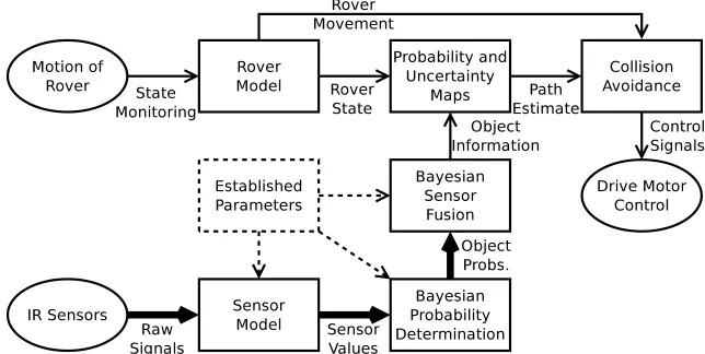
As a goal for a simple Bayesian sensing and control system, we construct an uncertainty map of the

rover’s surroundings that can be used to identify prominent features reliably and avoid collisions during forward motion. Figure 1 shows the flow of information through the system.

Figure 1. Bayesian Classification and Mapping Flowchart

II.A. Sensory Model

For the purposes of this study, the rover is tasked to observe all objects encountered and statistically identify obstacles. Infrared range sensors are used to detect objects based on infrared light reflected from their surfaces. Each sensor model is considered to be of a Bernoulli type with a probability of correct object detection βs, a fourth-order polynomial function of the sensor state s:6

s = _||X ₋X¯_|| (1) with ¯X being the rover’s location and X being the location of a sensed object. The probability of a range observation r given state s is considered to be:

βs =

Ms

ρs4

(s2 ₋ρs2) if s ≤ ρs

βs = 0.5 if s > ρs (2) where ρs is the sensor’s maximum range, beyond which correct and incorrect object detection are equally likely. Ms is used to set the peak value of βs if the object being observed is located at ¯X.

II.B. Bayesian Identification

A Bayesian method is used to update the probability of object presence given the probability of a range observation r. We define an estimation of the likelihood of encountering an object at location X and time

t + 1 as P(s_|r, X, t+ 1). Because no other reference besides the range sensors are used, a simple threshold 0 < Ss < ρs is applied to s such that Ss is beyond the measured noise level of the device, and an object is assumed to be present if s > Ss at time t. By applying Bayes’ rule, the probability of an object being found at the location X can be written in the form:7

P(s_|r, X, t+ 1) = P(r|s, X, t)P(s, X, t)

P(r, X, t) = βsP(s, X, t)

2βsP(s, X, t)−βs −P(s, X, t) + 1

if s > Ss (3) (1₋βs)P(s, X, t)

The object likelihood at X is then recorded in the rover’s map. If data already exists at X, the likelihoods are averaged, as several measurements are generally taken at a time.

The uncertainty in a measurement can be modelled as the informational entropy present.8 The informa-tion entropy at X and time t for a Bernoulli distribution Ps={Ps,1−Ps} are calculated as:

H(s_|r, X, t) = min

t (−P(s, X, t) ln(P(s, X, t))−(1−P(s, X, t)) ln(1−P(s, X, t))) (5) The minimum of all measurements over t taken at a mapped point X is used to reinforce that uncertainty decreases over time as more data is gathered.

II.C. Sensor Fusion

Three directional infrared sensors are placed on the front of the rover, with the side sensors angled 30◦ _out from the central sensor. To improve the detection reliability of objects in the probability map, the sensor data is combined using a linear opinion pool. Each sensor set at an angle θs is assumed to have a sensor angle of view Ws and a Gaussian horizontal detection likelihood, so the detection probability incorporating angular deviation for each sensor is estimated as:

αs =

1

W2

s

√

2π ∗e

−(Wsθs )2 (6)

The net opinion pool can then be described for N sensors at angles of θn with respect to a primary direction by:

P(s_|r, X, t, θ1, θ2,· · ·θN) = N X

n=1

P(s_|r, X, t)_∗ 1

W2

s

√

2π ∗e

−(Wsθn )2 (7)

II.D. Search Methodology

The rover maintains two maps of its operating area, one for detected object probability P(s_|r, X) and one for accumulated entropy H(s_|r, X), which are constant over t unless sensory data is added at any point

X. Mapping of object probabilities is done at each point X within the sensor range ρs of ¯X at the angle

θs. The map is split into cells, and assuming the rover is present at the centroid of cell X(x, y) then a sensor reading at range r will affect positions P(Xx +rcos(θs), Xy +rsin(θs)) are mapped for each sensor. Entropy is mapped in much the same way, as H(Xx + rcos(θs), Xy + rsin(θs)) for orthogonal Cartesian components Xx and Xy for each θs. Before any data is gathered, the probability map is initialized to 0, while the entropy map is normally initialized to 1 at every point. As the search process within the map is not generally randomized, this leads to the same pattern being repeated initially. To evaluate the impact of varying initial uncertainty on the search pattern, the entropy map was also initialized using a pseudo-random value δh < 1 as 1 − δh < H(X) < 1 in a separate set of tests. For efficiency, the rover is assumed to only evaluate a local area of radius Ds in its stored map at any given time t. Mapping continues until there are no remaining points with uncertainty exceeding a given threshold, _∀X_|H(X)< Hdesired.

Considering the set ∆s as all points within this radius, where {∀X ∈ ∆s,||X − X¯|| < Ds}, the target location ˆX is generally chosen to be the point with maximum uncertainty:

ˆ

X′ _{= arg max}

∆s

(H(s_|r, X)) (8)

However, as this typically results in mapping behaviour that follows the numerical map search algorithm, it is desirable to provide a more optimal search metric. We choose the map location with maximum uncertainty within the margin δh and minimum distance from the rover and use a logical OR with Eq. 8 in the algorithm:

ˆ

X = ˆX′ _{∨[arg max}

∆s

(H(s_|r, X)₋δh)∧arg min

∆s ||

X ₋X¯_||] (9)

II.E. Navigational Decisions

For forward navigation, we define the three sensor angles with respect to the forward direction as θL = −π/6,

θC = 0, θR = π/6. Once the area in front of the rover has been mapped, a most probable explanation methodology is used to determine the most appropriate course of action.9 Different courses of action are quantified by pre-coded “behaviours” that in this case are each defined with a set of conditions on the calculated posterior probabilities as:

BN := ∀s|s > Ss := “proceed normally′′ (10)

BSR := (P(s|r, X, θL) > P(s|r, X, θC))∧(P(s|r, X, θL)> P(s|r, X, θR)) := “slow turn right′′ (11)

BSL := (P(s|r, X, θR) > P(s|r, X, θC)) ∧(P(s|r, X, θR)> P(s|r, X, θL)) := “slow turn lef t′′ (12)

BQR := (P(s|r, X, θC) > P(s|r, X, θL))∧(P(s|r, X, θL) > P(s|r, X, θR)) := “quick turn right′′ (13)

BQL := (P(s|r, X, θC)> P(s|r, X, θL))∧(P(s|r, X, θL) > P(s|r, X, θR)) := “quick turn lef t′′ (14)

Normal mapping behaviour is continued until any object is considered to be detected, and then the obstacle avoidance behaviours are initiated. As the behaviour conditions are mutually exclusive, only one behaviour can be selected from the set B = _{BN, BSR, BSL, BQR, BQL}.

III.

Testing Results

III.A. Micro-Rover Platform

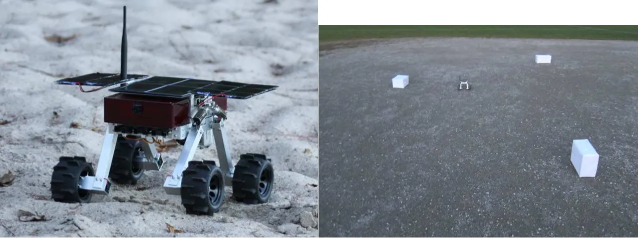
The Beaver micro-rover (or µrover) is used for testing of the Bayesian algorithm.10 The Beaver is a stand-alone, self-powered, autonomous ground roving vehicle under development at York University in Canada for the Northern Light mission, a Canadian initiative to send one or more landers to the surface of Mars to study the Martian environment.11 It is powered from solar panels and can recharge outdoors while operating, or by powering down onboard systems for extended periods. It has a power-efficient ARM-based onboard computer, a colour CMOS camera, magnetometer, accelerometer, GPS unit with DGPS capability, six navigational infrared sensors, and communicates via 900MHz ZigBee mesh networking. Capacity for two payloads is available in the current chassis design, and payloads that are planned include an infrared spectrometer, a rock drill, and a manipulator arm. A variety of communications interfaces including RS-485 serial, SPI, I2C, Ethernet and USB are used for payload interfacing.12 A design diagram and a picture of the Beaver µrover are shown in Figure 2. Programming is done in the C language using fixed-point numerical processing for efficiency.

Figure 2. Beaver Prototype Testing in Sand and in Outdoor Test Area with Obstacles

III.B. Navigational Results

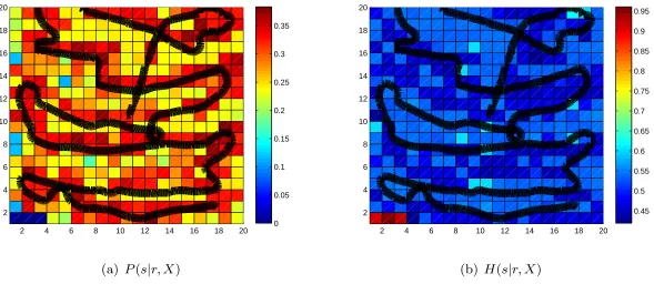
strategy detailed above, the rover was allowed to move freely in an area with no obstacles. For this test,

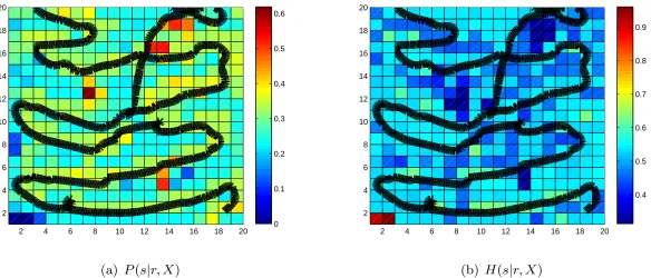
Ds = 8m, Ms = 0.5, and Ss = 0.75. First, each cell in the probability map was initialized to 0 and each in the entropy map was initialized to 1. Figure 3 shows the probability and uncertainty maps. The path that the rover took during the test is shown as an overlaid black line. The initial entropy map was then modified with a pseudo-random offset as suggested above with δh = 0.1. Figure 4 shows the probability and uncertainty maps. The new path that the rover chose is shown.

2 4 6 8 10 12 14 16 18 20 2 4 6 8 10 12 14 16 18 20 0.15 0.2 0.25 0.3 0.35 0.4

(a) P(s|r, X)

2 4 6 8 10 12 14 16 18 20 2 4 6 8 10 12 14 16 18 20 0.42 0.44 0.46 0.48 0.5 0.52 0.54 0.56 0.58 0.6 0.62

(b) H(s|r, X)

Figure 3. Probability and Uncertainty Maps, No Obstacles

2 4 6 8 10 12 14 16 18 20 2 4 6 8 10 12 14 16 18 20 0 0.05 0.1 0.15 0.2 0.25 0.3 0.35

(a) P(s|r, X)

2 4 6 8 10 12 14 16 18 20 2 4 6 8 10 12 14 16 18 20 0.45 0.5 0.55 0.6 0.65 0.7 0.75 0.8 0.85 0.9 0.95

(b) H(s|r, X)

Figure 4. Probability and Initially-Randomized Uncertainty Maps, No Obstacles

Three obstacles were then placed in the 20m by 20m area to test the obstacle avoidance methodology. The layout of the testing area used is shown in Figure 2. The rover was run with the same parameters as the tests above with the uncertainty map initialized to 0 and the entropy map initialized to 1. The resulting path and maps are shown in Figure 5. The test was repeated with the pseudo-random offset as suggested above with δh = 0.1, and the results are shown in Figure 6.

III.C. Discussion of Results

uncertainty initialization caused a shorter and less regular pattern indicating that the closest point search in Eq. 9 was dominant. In both cases, it is evident that the obstacles are detected as peaks in the probability map and successfully avoided, although due to the high granularity of the mapping, the obstacle location accuracy is quite coarse. No comparison was done in this study between different test areas and obstacle layouts, and it is possible that a less predictable path could be desired. In this case, greater randomization in the algorithm would likely suffice.

2 4 6 8 10 12 14 16 18 20 2 4 6 8 10 12 14 16 18 20 0.15 0.2 0.25 0.3 0.35 0.4 0.45 0.5 0.55 0.6

(a) P(s|r, X)

2 4 6 8 10 12 14 16 18 20 2 4 6 8 10 12 14 16 18 20 0 0.1 0.2 0.3 0.4 0.5 0.6

(b) H(s|r, X)

Figure 5. Probability and Uncertainty Maps, With Obstacles

2 4 6 8 10 12 14 16 18 20 2 4 6 8 10 12 14 16 18 20 0 0.1 0.2 0.3 0.4 0.5 0.6

(a) P(s|r, X)

2 4 6 8 10 12 14 16 18 20 2 4 6 8 10 12 14 16 18 20 0.4 0.5 0.6 0.7 0.8 0.9

(b) H(s|r, X)

Figure 6. Probability and Initially-Randomized Uncertainty Maps, With Obstacles

IV.

Conclusions

References

1

Schenker, P., “Advances in rover technology for space exploration,” Aerospace Conference, 2006 IEEE, 2006.

2

Giuseppe Della Penna, Benedetto Intrigila, D. M. F. M., “Resource-Optimal Planning For An Autonomous Planetary Vehicle,” International Journal of Artificial Intelligence and Applications, Vol. 1, No. 3, 2010, pp. 15 – 29.

3

Tara Estlin, Daniel Gaines, C. C. F. F. R. C. M. J. R. C. A. and Nesnas, I., “Enabling Autonomous Rover Science Through Dynamic Planning and Scheduling,” IEEE Aerospace Conference (IAC 05). Big Sky, MT. March 2005, 2011.

4

Huntsberger, T., “Onboard Learning of Adaptive Behavior: Biologically Inspired and Formal Methods,” Advanced Tech-nologies for Enhanced Quality of Life Conference, 2009, pp. 152 – 157.

5

Gallant, M., Ellery, A., and Marshall, J., “Science-influenced mobile robot guidance using Bayesian Networks,” Electrical and Computer Engineering (CCECE), 2011 24th Canadian Conference, 8-11 May 2011, pp. 001135 – 001139.

6

Hussein, I. I. and Stipanovic, D. M., “Effective Coverage Control for Mobile Sensor Networks With Guaranteed Collision Avoidance,” IEEE Transactions on Control System Technology, Vol. 15, No. 4, 2007, pp. 642–657.

7

Wang, Y. and Hussein, I. I., “Bayesian-Based Decision Making for Object Search and Classification,” IEEE Transactions on Control Systems Technology, Vol. 19, No. 6, 2011, pp. 1639–1647.

8

Wang, Y. and Hussein, I. I., “Intentional Control for Planetary Rover SRR,” American Control Conference (ACC), 2011, June 29-July 1 2011, pp. 1280 – 1285.

9

Koller, D. and Friedman, N., Probabilistic Graphical Models, Principles and Techniques, MIT Press, Cambridge, Mas-sachusetts, 2009.

10

Post, M. A., L. R. and Quine, B. M., “Beaver Micro-Rover Development For The Northern Light Mars Lander,” Con-ference Proceedings of CASI ASTRO 2012. Chateau Frontenac, Quebec City, Canada, April 2012.

11

Quine, B., Lee, R., and Roberts, C. e. a., “Northern Light - A Canadian Mars Lander Development Plan,” Conference Proceedings of CASI ASTRO 2008, Montreal, Canada, 2008.

12