Nonlinear evolution of the electromagnetic electron-cyclotron instability in bi-Kappa distributed plasma

Nonlinear evolution of the electromagnetic electron-cyclotron instability

in bi-Kappa distributed plasma

B.Eliasson1,a)and M.Lazar2,3,b) 1

SUPA, Physics Department, John Anderson Building, Strathclyde University, Glasgow G4 0NG, Scotland, United Kingdom

2

Centre for Mathematical Plasma Astrophysics, Celestijnenlaan 200B, 3001 Leuven, Belgium 3

Institut f€ur Theoretische Physik, Lehrstuhl IV: Weltraum- und Astrophysik, Ruhr-Universitat Bochum,€ 44780 Bochum, Germany

(Received 6 May 2015; accepted 26 May 2015; published online 15 June 2015)

This paper presents a numerical study of the linear and nonlinear evolution of the electromagnetic electron-cyclotron (EMEC) instability in a bi-Kappa distributed plasma. Distributions with high energy tails described by the Kappa power-laws are often observed in collision-less plasmas (e.g., solar wind and accelerators), where wave-particle interactions control the plasma thermodynamics and keep the particle distributions out of Maxwellian equilibrium. Under certain conditions, the anisotropic bi-Kappa distribution gives rise to plasma instabilities creating low-frequency EMEC waves in the whistler branch. The instability saturates nonlinearly by reducing the temperature ani-sotropy until marginal stability is reached. Numerical simulations of the Vlasov-Maxwell system of equations show excellent agreement with the growth-rate and real frequency of the unstable modes predicted by linear theory. The wave-amplitude of the EMEC waves at nonlinear saturation is consistent with magnetic trapping of the electrons.VC _{2015 Author(s). All article content, except}

where otherwise noted, is licensed under a Creative Commons Attribution 3.0 Unported License.

[http://dx.doi.org/10.1063/1.4922479]

I. INTRODUCTION

Direct in-situ measurements in space plasmas reveal

particle distributions far from thermal (Maxwellian) equilib-rium by the presence of suprathermal populations that enhance the high-energy tails of the distribution functions, as well as kinetic anisotropies manifested as a temperature ani-sotropyT?=Tk6¼1 of the electron and proton velocity distri-butions (where the perpendicular and parallel directions are with respect to the direction of the ambient magnetic field), and sometimes as beam-like features.1Particle-particle colli-sions are indeed rare in space plasmas and cannot establish thermal equilibrium, but wave-particle interactions can reso-nantly accelerate part of the particle population and explain the deviations from Maxwellian equilibrium. However, these anisotropies are not as high as expected from exospheric models, and hence there seems to be a limiting factor on the temperature anisotropy.2,3In the absence of collisions, linear theory predicts that temperature anisotropy driven instabil-ities could lead to a partial thermalization of the particles until marginal stability is reached. For electrons, an excess of temperature in the parallel directionTk>T? can be lim-ited by the firehose instability, while an excess temperature in the perpendicular direction T?>Tk is limited by the whistler instability, also known as the electromagnetic elec-tron cycloelec-tron (EMEC) instability.2For a sufficiently small electron plasma beta, i.e., b<0:1, the EMEC instability is competed by electrostatic instabilities propagating obliquely to the magnetic field,4,5or by the slow extraordinary mode

(Z mode) that becomes unstable when the electron gyro-frequency is larger than the electron plasma gyro-frequency.4

Whistler waves propagating along the magnetic field lines are right-hand circularly polarized electromagnetic waves with frequencies between the ion and electron cyclo-tron frequencies and were first observed in ionospheric physics.6Low-frequency whistler waves triggered by light-nings in the Earth’s equatorial region have frequencies in the kilohertz range and propagate between the hemispheres with a descending whistler-like tone. On the other hand, whistler waves triggered by electron anisotropies and suprathermal populations of electrons are expected to play an important role at dissipative scales in the solar wind7 and planetary magnetospheres.8,9 Whistler instabilities have also been observed in laboratory experiments.10

In the first investigations of the EMEC instability, the anisotropic electrons were described by idealized bi-Maxwellian models (see the textbook of Gary11and referen-ces therein), while more recently, the EMEC instability has been studied using generalized power-laws, such as bi-Kappa or product-bi-Kappa models, which incorporate suprathermal electrons in the distribution functions.12–17 A variety of plasma parameters have also been invoked, ranging from the weakly magnetized plasma of the solar wind, via the moder-ately magnetized plasmas of the coronal outflows, flares, and the plasma sheet, to the highly magnetized plasmas in the tail lobe and the radiation belts in the magnetosphere. Compared to the case with bi-Maxwellian electrons (recovered in the limit of a very large power-index j! 1), the influence of suprathermal populations on the EMEC instability was found to be highly dependent on the shape of the velocity distribu-tion as well as the temperature anisotropy. For bi-Kappa

a)_{Electronic mail: [email protected]}

b)

Electronic mail: [email protected]

distributed electrons with perpendicular temperature much higher than parallel temperature, the growth-rate tends to increase with increasing the kappa-index,13,14while the oppo-site holds at a low temperature anisotropy.12 On the other hand, the lowest thresholds relevant for the marginal instabil-ity condition decrease with increasing the densinstabil-ity of supra-thermal populations.15

Large amplitude whistlers can undergo dual cascades to both larger and smaller wavenumbers involving parametric processes.18A spectrum of waves can change the background electron distribution function via quasilinear and other nonlin-ear processes.19,20Introduced first for an arbitrary distribution of plasma particles,22,23 the quasilinear approach has been specialized and tested for bi-Maxwellian distributed plas-mas,21,24,25showing that the increase of the EMEC magnetic fields tends to decrease the temperature anisotropy to a point of marginal stability. Similar results were found in particle-in-cell simulations using a Maxwellian dense core and highly temperature anisotropic (T?=Tk¼25) bi-Kappa distributed tails.26Using a set of conserved quantities for whistler waves propagating parallel to the magnetic field,23 it is possible to show that an increase of the wave magnetic field energy leads to an increase of the total parallel kinetic energy and a decrease of the perpendicular kinetic energy of the electrons, while conserving the total energy of the system.

The aim of this paper is to numerically investigate linear growth and nonlinear saturation of the EMEC instability in a bi-Kappa distributed plasma, and to compare the results with the existing theoretical predictions and simulations. In Sec. II, we provide a brief mathematical formulation for the bi-Kappa model invoked and the resulting dispersion relations of the EMEC modes. We restrict to EMEC modes propagat-ing parallel (k¼kk) to the magnetic field, because in parallel direction these modes exhibit maximum growth rates and

decouple from the electrostatic modes.27 The simulation

setup and the principal results are presented to a large detail in Sec.III. The simulations are based on a previously devel-oped Vlasov-Maxwell solver that uses a Fourier transform technique in velocity space to solve the Vlasov equation.31,32 The numerical code, which showed excellent agreement with theory for the whistler instability with a bi-Maxwellian electron distribution,31,32is here extended to study the more general case of a bi-Kappa distribution function for the elec-trons. Similarities and differences between the simulation results and previous results using the bi-Maxwellian electron distributions are discussed in detail. The main conclusions of our study are iterated in Sec.IV.

II. MATHEMATICAL FORMULATION

In preparation for the numerical simulations, we assume a geometry of the problem in which the background mag-netic field is directed along thez-axis,B0¼^zB0, whereB0is the magnitude of the magnetic field and ^z is a unit vector along thez-axis. The fluctuating electric and magnetic fields,

f vð k;v?Þ ¼ 1

p3=2_h2

?hk

Cðjþ1Þ

j3=2_Cðj1=2Þ 1þ

v2

k

jh2_kþ

v2

?

jh2_?

!j1 ;

(1)

where j is the power index, the perpendicular and parallel (to the magnetic field) velocity components are denoted

v?¼

ffiffiffiffiffiffiffiffiffiffiffiffiffiffi

v2

xþv2y q

and vk¼vz, respectively, and the parallel

and perpendicular thermal speeds hk and h? are defined in terms of the respective kinetic temperatures Tk and T? via the relations (see, e.g., Ref.15)

Tk¼

meh2_k 2kB

j

j3=2; (2)

and

T?¼

meh2_? 2kB

j

j3=2: (3)

The linear dispersion relation for the instability of EMEC-whistler waves propagating along the background magnetic field for a bi-Kappa distribution (omitting subscript kfor the wavenumberk) reads (see, e.g., Ref.15)

k2_c2

x2

p ¼T?

Tk

1þ ðxxceÞT?=Tkþxce

kpffiffiffiffiffiffiffiffiffiffiffiffiffiffiffiffiffiffiffiffi2kBTk=me

ffiffiffiffiffiffiffiffiffiffiffiffiffiffiffiffiffiffiffiffiffiffi 13=ð2jÞ p

Zj

xxce

k ffiffiffiffiffiffiffiffiffiffiffiffiffiffiffiffiffiffiffiffi2kBTk=me

p ffiffiffiffiffiffiffiffiffiffiffiffiffiffiffiffiffiffiffiffiffiffi 13=ð2jÞ p

; (4)

in terms of the dispersion function for a bi-Kappa distributed plasma28

Zjð Þ ¼n

1

p1=2_j1=2

Cð Þj

Cðj1=2Þ ð1

1

dx 1þx

2_=j

j

xn ;Ið Þn >0:

(5)

In the limit j¼ 1, the bi-Kappa distribution converges to the bi-Maxwellian distribution function, and the dispersion relation can be written29

k2_c2

x2 pe

¼T?

Tk

1þðxxceÞT?=Tkþxce

k ffiffiffiffiffiffiffiffiffiffiffiffiffiffiffiffiffiffiffiffi2kBTk=me

p Z xxce

k ffiffiffiffiffiffiffiffiffiffiffiffiffiffiffiffiffiffiffiffi2kBTk=me p

;

(6)

where

ZðnÞ ¼ipffiffiffipexpðn2Þ½1þerfðinÞ; (7)

is the plasma dispersion function30 and erfðzÞ is the error function of complex arguments.

the ions are assumed to be immobile. The initial condition for the electron distribution function is obtained by using the Fourier transform pair in velocity space

fðx;v;tÞ ¼ ð

^

fðx;g;tÞeigvd3g; (8)

^

fðx;g;tÞ ¼ 1 2p

ð Þ3 ð

fðx;v;tÞeigvd3v; (9)

which yields the Fourier transformed bi-Kappa distribution function

^

f_ðg_k;g_{?Þ ¼} 2

2p

ð Þ3

n

2

j1=2

Kj1=2ð Þn

Cðj1=2Þ; (10)

where n¼ ffiffiffiffiffiffiffiffiffiffiffiffiffiffiffiffiffiffiffiffiffiffiffiffiffiffiffiffiffiffiffijh2_kg2

kþjh

2

?g2? q

, g is the Fourier transformed

velocity variable, CðnÞis the Gamma function of argument

n, andKvðnÞis the modified Bessel function of second kind of non-integer ordervand argumentn.33The normalization Ð

f d3_{v¼1 corresponds to f^}

g¼0¼1=ð2pÞ 3

in the Fourier transformed velocity space.31,32 More details of the simula-tion set-up are given in the Appendix. It has been confirmed that the simulations conserve the total energy to a high degree in the nonlinear evolution of the system: While the magnetic wave energy increases to about 3%–5% of the total (kinetic plus electromagnetic) energy and the electron kinetic energy decreases with approximately the same amount, the total energy typically decreases by about 0.1%. The electric energy is only about 0.01% as expected for low-frequency whistlers withxce=xpe1.

We have carried out three sets of simulations, (i) where the initial electron number density and magnetic field are

chosen such that xpe=xce¼12:65, using a relatively large temperature anisotropyT?=Tk¼8, (ii) for a larger density rel-ative to the magnetic field such that xpe=xce ¼40 and

T?=Tk¼8, and finally (iii)xpe=xce¼40 and a lower tem-perature anisotropyT?=Tk¼4. In all cases, we use an electron temperature such thatkBTk=mec2¼1=2500, corresponding to

Tk ¼2:37 MK. These plasma parameters are typical for the conditions in the solar corona, solar wind, and solar flares; see, e.g., Refs.14,34, and35. The parallel electron plasma beta

b_k ¼2n0kBTkl0

B2 0

¼2kBTk

mec2

x2

pe

x2

ce

; (11)

takes the value 0.128 in case (i) and 1.28 in cases (ii) and (iii). Theoretical and numerical investigations using bi-Maxwellian electron velocity distributions5have shown that the instability has the largest growth-rate in the parallel direction forbk >0:025, while forbk <0:025 the instability has larger growth-rates at large angles giving rise to waves with large electrostatic components. For the selected parame-ters, withbk>0:1, it is therefore expected that the instabil-ity has a maximum growth rate in the parallel direction, consistent with the simulation geometry.

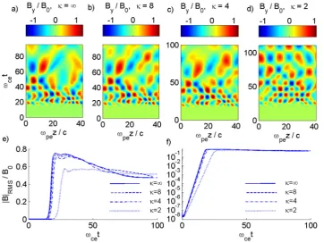
Figures 1–3 show the spatiotemporal evolution of the

wave magnetic field forj¼ 1(i.e., a bi-Maxwellian distri-bution), j¼8,j¼4, and j¼2 for the three cases (i)–(iii). The unstable EMEC wave modes initially grow exponen-tially with time and saturate nonlinearly after the initial small-amplitude perturbations have increased about 8 orders of magnitude in amplitude. The resulting large amplitude right-hand polarized whistler-like EMEC waves are visible in panels (a)–(d). As seen in panels (e) and (f), the most unstable mode grows faster and the saturation amplitude is larger for larger values ofj. The amplitude of the wave field

FIG. 1. The spatiotemporal evolution of the wave magnetic field, showing the nonlinear saturation of the EMEC instability by large amplitude waves for xpe=xce¼12:65;T?=Tk¼8, and

typically reaches a maximum as the linear growth saturates, and for the cases of higher plasma beta shown in Figs.2and

3 [panels (a)–(d)], the wave field at later times slowly

decreases in amplitude as the wave spectrum cascades to lon-ger wavelengths. A similar effect was observed in Ref.25in the form of a saturation and switching off of the growth of shorter wavelength waves and a shift of the unstable wave spectrum to longer wavelengths. The case of smaller temper-ature anisotropy shown in Fig. 3 gives lower growth-rates

and saturation amplitudes compared to the higher anisotropy case in Fig.2.

Figures4–6show the growth-rates and real frequencies obtained in the Vlasov simulations, and a comparison with the theoretical values obtained from the wave dispersion relations (4) and (6). The numerical values of the real fre-quency were obtained by studying the periodicity of the exponentially growing wave mode in time for each value of the wavenumber, while the growth-rates were obtained by

FIG. 2. The spatiotemporal evolution of the wave magnetic field, showing the nonlinear saturation of the EMEC instability by large amplitude waves forxpe=xce¼40;T?=Tk¼8, and (a)

j¼ 1, (b)j¼8, (c) j¼4, and (d) j¼2. (e) The time evolutions of the root mean square magnetic field, and the same data are plotted in (f) with logarithmic scale on the vertical axis.

FIG. 3. The spatiotemporal evolution of the wave magnetic field, showing the nonlinear saturation of the EMEC instability by large amplitude waves forxpe=xce¼40;T?=Tk¼4, and (a)

linear fits (linear regression) in time to the logarithm of the amplitude of each mode during its linear growth phase. As

seen in Figs. 4–6, the growth-rates and real frequencies

obtained in the Vlasov simulations agree very well with the theoretical dispersion curves, which give confidence in the correctness of both the theoretical and numerical results. The

modes with the highest growth-rates in Figs. 4–6 are the

dominating mode first visible and saturating nonlinearly in

Figs. 1–3. Also in agreement with Figs. 1–3, the

growth-rates of the fastest growing modes are larger for larger values ofj, while the wavenumber and hence the wavelength of the fastest growing modes are only weakly dependent onj. The ambient magnetic field has in general a stabilizing effect on

the EMEC instability, and the spectrum of unstable wave modes shrink with increasing magnetic field. This effect can be observed in the low-beta case in Fig.4, where the smallest wavenumbers (e.g.,kc=xpeⱗ0:5) are stabilized compared to the high-beta cases in Figs.5and6. On the other hand, for a smaller spectral indexj¼2, the smaller wavenumber modes also become unstable, as seen in Fig.4(g). As expected, the case of smaller temperature anisotropy in Fig. 7also gives smaller growth-rates and a narrower range of unstable modes of the EMEC instability compared to Fig.6. This is consist-ent with the condition kc=xpe ðT?=Tk1Þ1=2 for a bi-Maxwellian plasma,22,25 which also leads to a stabilization of the higher wavenumber modes as the temperature

FIG. 4. Growth-rates (top panels) and corresponding real frequencies (bottom panels) of the EMEC instability obtained in the Vlasov simulation (“þ” markers) and the theoretical growth values (solid lines) for xpe=xce ¼12:65;T?=Tk¼8;j¼ 1 [(a) and

(b)],j¼8 [(c) and (d)],j¼4 [(e) and (f)], andj¼2 [(g) and (h)]. The maxi-mum growth-rate isxI=xce¼0:32 at kc=xpe¼1:2 for j¼ 1, xI=xce ¼0:31 at kc=xpe¼1:2 for j¼8,

xI=xce¼0:29 at kc=xpe¼1:2 for

j¼4, and xI=xce¼0:22 at kc=xpe ¼1:2 forj¼2.

FIG. 5. Growth-rates (top panels) and corresponding real frequencies (bottom panels) of the EMEC instability obtained in the Vlasov simulation (“þ” markers) and the theoretical growth values (solid lines) for xpe=xce ¼40;T?=Tk¼8;j¼ 1 [(a) and

(b)],j¼8 [(c) and (d)],j¼4 [(e) and (f)], andj¼2 [(g) and (h)]. The maxi-mum growth-rate isxI=xce¼1:09 at kc=xpe¼1:1 for j¼ 1, xI=xce ¼1:06 at kc=xpe¼1:1 for j¼8,

xI=xce¼1:01 at kc=xpe¼1:1 for

anisotropy decreases. For all cases, the most unstable wave modes have real frequencies somewhat below the electron cyclotron frequency,xR0:70–0:75xce. By comparing the results in Figs.1–3with Figs.4–6, it is interesting to notice that the maximum amplitude of the wave magnetic field as the instability saturates nonlinearly increases with the maxi-mum linear growth-rate. Similar results were obtained in Refs.22and24and were explained by magnetic trapping of electrons.

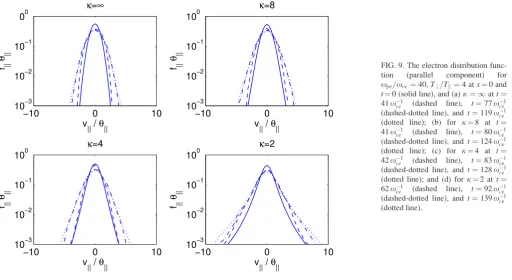
Figures7–9show the time evolution of the parallel elec-tron distribution function, defined as the elecelec-tron distribution

function integrated over the perpendicular velocity space,

fk ¼Ðfd2v?. Att¼0 (the solid lines in Figs.7–9), we have from Eq.(1)

fkð Þ ¼vk 1

p1=2_h

k

Cðjþ1Þ

j3=2_Cðj1=2Þ 1þ

v2

k

jh2_k

!j

: (12)

In general, the electron distribution function shows a broad-ening in the parallel direction until marginal stability is reached. The broadening in the parallel direction is

FIG. 6. Growth-rates (top panels) and corresponding real frequencies (bottom panels) of the EMEC instability obtained in the Vlasov simulation (“þ” markers) and the theoretical growth values (solid lines) for xpe=xce ¼40;T?=Tk¼4;j¼ 1 [(a) and

(b)],j¼8 [(c) and (d)],j¼4 [(e) and (f)], andj¼2 [(g) and (h)]. The maxi-mum growth-rate is xI=xce¼0:5 at kc=xpe¼0:85 for j¼ 1, xI=xce ¼0:48 at kc=xpe¼0:84 for j¼8,

xI=xce¼0:45 at kc=xpe¼0:80 for

j¼4, and xI=xce¼0:33 at kc=xpe ¼0:80 forj¼2.

FIG. 7. The electron distribution func-tion (parallel component) for xpe=xce¼12:65, T?=Tk¼8 at x¼0

andt¼0 (solid line), and (a)j¼ 1at

t¼65x1

ce (dashed line),t¼118x 1 ce

(dashed-dotted line), andt¼172x1 ce

(dotted line); (b) for j¼8 at

t¼65x1

ce (dashed line),t¼121xce1

(dashed-dotted line), andt¼178x1 ce

(dotted line); (c) for j¼4 at

t¼68x1

ce (dashed line),t¼124xce1

(dashed-dotted line), andt¼180x1 ce

(dotted line); and (d) for j¼2 at t¼122x1

ce (dashed line), t¼163x1

ce (dashed-dotted line), and t¼203x1

indicative of wave-particle interactions via quasi-linear proc-esses. For parallel propagation of the whistler waves, two conserved quantities23,25ensure that an increase of magnetic wave energy leads to the simultaneous increase of parallel kinetic energy and decrease of perpendicular kinetic energy. Hence, the growth of whistler waves due to the EMEC insta-bility leads to a broadening of the electron velocity distribu-tion in the parallel direcdistribu-tion (as seen in Figs. 7–9) and narrowing in the perpendicular direction until marginal stability is achieved. In a similar way as in Ref. 25 for a

bi-Maxwellian plasma, when the anisotropy decreases, the electro distribution does not change the shape, remaining in this case approximately Kappa distributed. Thermal spread increases in parallel direction but, apparently, the high-energy tails are diminished (increasing of the power index

j). In general, the present results are also in line with more

recent simulations26 using a dense core (95% density)

Maxwellian distribution and a low-density (5% density) bi-Kappa distributed halo with T?=Tk¼25, but in the latter case a decrease ofjwas instead observed.

FIG. 8. The electron distribution func-tion (parallel component) for xpe=xce¼40,T?=Tk¼8 atx¼0 and t¼0 (solid line), and (a)j¼ 1att ¼28x1

ce (dashed line), t¼58xce1

(dashed-dotted line), and t¼96x1 ce

(dotted line); (b) for j¼8 at

t¼29x1

ce (dashed line), t¼59x 1 ce

(dashed-dotted line), and t¼96x1 ce

(dotted line); (c) for j¼4 at t¼

30x1

ce (dashed line), t¼62xce1

(dashed-dotted line), andt¼103x1 ce

(dotted line); and (d) forj¼2 att¼

46x1

ce (dashed line), t¼70xce1

(dashed-dotted line), andt¼111x1 ce

(dotted line).

FIG. 9. The electron distribution func-tion (parallel component) for xpe=xce¼40,T?=Tk¼4 atx¼0 and t¼0 (solid line), and (a)j¼ 1att¼

41x1

ce (dashed line), t¼77x 1 ce

(dashed-dotted line), andt¼119x1 ce

(dotted line); (b) for j¼8 at t¼

41x1

ce (dashed line), t¼80xce1

(dashed-dotted line), andt¼124x1 ce

(dotted line); (c) for j¼4 at t¼

42x1

ce (dashed line), t¼83xce1

(dashed-dotted line), andt¼128x1 ce

(dotted line); and (d) forj¼2 att¼

62x1

ce (dashed line), t¼92xce1

(dashed-dotted line), andt¼139x1 ce

IV. CONCLUSIONS

We have studied the linear and nonlinear evolution of the EMEC instability for a collisionless anisotropic plasma by means of numerical simulations of the Vlasov-Maxwell system, using a bi-Kappa distribution for the electrons to model high-energy tails in their distribution. The numerically obtained growth-rates and real frequencies show excellent agreement with theoretical models. For a relatively large temperature anisotropy T?=Tk, the instability has largest growth-rate for large spectral indices (j! 1). The EMEC instability saturates nonlinearly by exciting large-amplitude right-hand circularly polarized electromagnetic waves with frequencies near the electron cyclotron frequency. The EMEC instability saturates by magnetic trapping of elec-trons,22,24,25leading to an increase of the saturated amplitude for higher linear growth-rates of the instability.

Values chosen for the plasma parameters in our numeri-cal setup are relevant for the hot plasma in the solar corona and flares, where the electron temperature typically is a few million Kelvin and the electron plasma frequency is about ten times higher than the electron cyclotron frequency. But extensions of the present results to the outer corona condi-tions in the solar wind and terrestrial magnetosphere are straightforward because the plasma beta in these environ-ments remains in the same range (e.g., 0:1<be<10 (Ref. 3)) as relevant in our simulations. Thus, the results obtained in the present paper provide major premises to approach more complex models of the solar wind particles, which combine a bi-Maxwellian core population at low energies and a bi-Kappa distribution modeling the supra-thermal component.16,17 The anisotropy of each component contributes to different peaks in the unstable spectrum, and the nonlinear evolution of these cases of high complexity may now be addressed in future works. Moreover, the nu-merical technique presented here may easily be adapted to enable further studies of other instabilities driven by kinetic anisotropies in Kappa distributed plasmas, for example, oblique generation of whistlers that would include quasi-electrostatic modes with a component of the electric field along the wave vector that could lead to efficient accelera-tion of the tail electrons to high energies.

ACKNOWLEDGMENTS

M.L. acknowledges support from the Katholieke

Universiteit Leuven, Grant No. SF/12/003, and from the Ruhr-Universit€at Bochum. These results were obtained in the framework of the Project Nos. GOA/2015-014 (KU Leuven) and C 90347 (ESA Prodex 9). The research leading to these results has also received funding from the European Commission’s Seventh Framework Programme (FP7/2007-2013) under the Grant Agreements SOLSPANET (Project

No. 269299, www.solspanet.eu) and eHeroes (Project No.

284461, www.eheroes.eu). B.E. acknowledges support from

APPENDIX: SIMULATION PARAMETERS AND SETUP

The simulation geometry is a one-dimensional simulation box in thez-direction, parallel to the ambient magnetic field. The simulation box is of size Lx¼ ð2p=0:15Þpc=xpe 41:9c=xpe and is resolved with 80 intervals with periodic boundary conditions. A pseudospectral method to calculate spatial derivatives accurately, and numerical dissipation is used at high wavenumbers to reduce aliasing effects. The three-dimensional velocity space is resolved by 767676 intervals, using a Fourier method31,32 and high-order differ-ence schemes to calculate derivatives in the Fourier trans-formed velocity space. To accurately resolve the evolution in the Fourier transformed velocity space, we use a maximum

gz;max¼6vTk1 for j¼ 1, gz;max¼7vTk1 for j¼8, gz;max ¼8v_Tk1 for j¼4, and gz;max¼10vTk1 for j¼2, and half these values, gx;max¼gy;max¼gz;max=2, in the perpendicular dimensions, where we denoted vTk¼ ffiffiffiffiffiffiffiffiffiffiffiffiffiffiffiffiffikBTk=me

p

. The maxi-mum represented velocity is given byvmax¼p=DgwhereDg is the grid size in the Fourier transformed velocity space, and the represented grid spacing in velocity space is given by Dv¼p=g_max. Therefore, the maximum represented parallel velocities are vz;max20vTk for j¼ 1;vz;max17vTk for

j¼8,vz;max15vTkforj¼4, andvz;max12vTk forj¼2, and twice as large represented velocities in the perpendicular

vxandvyvelocity dimensions where the anisotropic velocity

distributions are wider. To seed the instability, a quasi-random wave magnetic field is introduced in the initial condi-tions with an amplitude about 8 orders of magnitude smaller than the ambient magnetic field. Identical initial conditions for the wave magnetic field are used in all simulations. A 4th-order Runge-Kutta scheme is used to advance the solution in time, with adaptive time-stepping to maintain numerical sta-bility in the nonlinear evolution of the system. The number of time-steps used is 16 000.

1_{E. Marsch, “Kinetic physics of the solar corona and solar wind,”Living}

Rev. Sol. Phys.3, 1 (2006). 2

S. P. Gary and J. Wang, “Whistler instability: Electron anisotropy upper bound,” J. Geophys. Res. 101, 10749–10754, doi:10.1029/96JA00323 (1996).

3

S. Stverak, P. Travnicek, M. Maksimovic, E. Marsch, A. N. Fazakerley, and E. E. Scime, “Electron temperature anisotropy constraints in the solar wind,”J. Geophys. Res.113, A03103, doi:10.1029/2007JA012733 (2008). 4_{S. P. Gary and I. H. Cairns, “Electron temperature anisotropy instabilities:}

Whistler, electrostatic and z mode,” J. Geophys. Res. 104(A9), 19835–19842, doi:10.1029/1999JA900296 (1999).

5_{S. P. Gary, K. Liu, and D. Winske, “Whistler anisotropy instability at}

low electronb: Particle-in-cell simulations,”Phys. Plasmas18, 082902 (2011).

6_{R. A. Helliwell,Whistlers and Related Ionospheric Phenomena(Stanford} University Press, Stanford, CA, 1965).

7_{C. Lacombe, O. Alexandrova, L. Matteini, O. Santolik, N.}

Cornilleau-Wehrlin, A. Mangeney, Y. de Conchy, and M. Maksimovic, “Whistler mode waves and the electron heat flux in the solar wind: CLUSTER obser-vations,”Astrophys. J.796, 5 (2014).

8

associated and lightning-associated whistler waves in the Earths inner plasmasphere at L<2,” J. Geophys. Res. 116, A06310, doi:10.1029/ 2010JA016288 (2011).

10_{J. M. Urrutia, R. L. Stenzel, and K. D. Strohmaier, “Nonlinear electron}

magnetohydrodynamics physics. IV. Whistler instabilities,”Phys. Plasmas 15, 062109 (2008).

11

S. P. Gary,Theory of Space Plasma Microinstabilities(University Press, Cambridge, 1993).

12_{R. L. Mace, “Whistler instability enhanced by suprathermal electrons}

within the Earth’s foreshock,”J. Geophys. Res.103(A7), 14643–14654, doi:10.1029/98JA00616 (1998).

13_{R. L. Mace and R. D. Sydora, “Parallel whistler instability in a plasma}

with an anisotropic bi-Kappa distribution,”J. Geophys. Res.115, A07206, doi:10.1029/2009JA015064 (2010).

14

M. Lazar, S. Poedts, and R. Schlickeiser, “Instability of the parallel elec-tromagnetic modes in Kappa distributed plasmas—I. Electron whistler-cyclotron modes,”Mon. Not. R. Astron. Soc.410, 663–670 (2011). 15

M. Lazar, S. Poedts, and M. J. Michno, “Electromagnetic electron whistler-cyclotron instability in bi-Kappa distributed plasmas,” Astron. Astrophys.554, A64 (2013).

16_{M. Lazar, S. Poedts, and R. Schlickeiser, “The interplay of Kappa}

and core populations in the solar wind: Electromagnetic electron cy-clotron instability,” J. Geophys. Res.: Space Phys. 119, 9395–9406 (2014).

17_{M. Lazar, S. Poedts, R. Schlickeiser, and C. Dumitrache, “Towards}

realis-tic parametrization of the kinerealis-tic anisotropy and the resulting instabilities in space plasmas. Electromagnetic electron-cyclotron instability in the so-lar wind,”MNRAS446, 3022–3033 (2015).

18

S. P. Gary, R. S. Hughes, J. Wang, and O. Chang, “Whistler anisotropy instability: Spectral transfer in a three-dimensional particle-in-cell simu-lation,”J. Geophys. Res.: Space Phys.119, 1429–1434 (2014).

19_{A. A. Galeev and R. Z. Sagdeev,Nonlinear Plasma Theory(Benjamin,} New York, 1966).

20

V. I. Karpman, “Nonlinear effects in the ELF waves propagating along the magnetic field in the magnetosphere,” Space Sci. Rev. 16, 361–388 (1974).

21

P. H. Yoon, J. J. Seough, K. H. Kim, and D. H. Lee, “Empirical versus exact numerical quasilinear analysis of electromagnetic instabilities driven by temperature anisotropy,”J. Plasma Phys.78, 47–54 (2012).

22_{R. C. Davidson, D. A. Hammer, I. Haber, and C. E. Wagner, “Nonlinear}

development of electromagnetic instabilities in anisotropic plasmas,”

Phys. Fluids15, 317–333 (1972). 23

R. C. Davidson and D. A. Hammer, “Nonequilibrium energy constants associated with large-amplitude electron whistlers,” Phys. Fluids 15, 1282–1284 (1972).

24

S. L. Ossakow, I. Haber, and E. Ott, “Simulation of whistler instabilities in anisotropic plasmas,”Phys. Fluids15, 1538–1540 (1972).

25_{S. L. Ossakow, E. Ott, and I. Haber, “Nonlinear evolution of whistler}

instabilities,”Phys. Fluids15, 2314–2326 (1972). 26

Q. Lu, L. Zhou, and S. Wang, “Particle-in-cell simulations of whistler waves excited by an electronjdistribution in space plasma,”J. Geophys. Res.115, A02213, doi:10.1029/2009JA014580 (2010).

27_{C. F. Kennel and H. E. Petschek, “Limit on stably trapped particle fluxes,”}

J. Geophys. Res.71, 1–28, doi:10.1029/JZ071i001p00001 (1966). 28

D. Summers and R. M. Thorne, “The modified plasma dispersion function,”Phys. FluidsB3, 1835–1847 (1991).

29_{H. Stix,Waves in Plasmas(Springer-Verlag, New York, 1992).} 30

B. D. Fried and S. D. Conte,The Plasma Dispersion Function/The Hilbert transform of the Gaussian(Academic Press, New York, 1961).

31_{B. Eliasson, “Outflow boundary conditions for the Fourier transformed}

three-dimensional Vlasov-Maxwell system,” J. Comput. Phys. 225, 1508–1532 (2007).

32

B. Eliasson, “Numerical simulations of the Fourier transformed Vlasov-Maxwell system in higher dimensions—Theory and applications,”Transp. Theory Stat. Phys.39(5&7), 387–465 (2010).

33

The modified Bessel function of the second kind for non-negative argu-ment and non-negative order is calculated numerically using the Fortran 77 routine RKBESL, seehttp://www.netlib.org/specfun/rkbesl.

34_{R. A. Treumann and W. Baumjohann,Advanced Space Plasma Physics} (Imperial College Press, London, 1997).

35