arXiv:1502.02577v2 [physics.soc-ph] 22 Mar 2015
Random Rectangular Graphs
Ernesto Estrada and Matthew Sheerin
A generalization of the random geometric graph (RGG) model is proposed by considering
a set of points uniformly and independently distributed on a rectangle of unit area instead of
on a unit square[0,1]2.The topological properties of therandom rectangular graphs(RRGs)
generated by this model are then studied as a function of the rectangle sides lengths aand
b= 1/a, and the radius rused to connect the nodes. Whena= 1we recover the RGG, and
whena→ ∞the very elongated rectangle generated resembles a one-dimensional RGG. We
obtain here analytical expressions for the average degree, degree distribution, connectivity,
average path length and clustering coefficient for RRG. These results provide evidence that
show that most of these properties depend on the connection radius and the side length
of the rectangle, usually in a monotonic way. The clustering coefficient, however, increases
when the square is transformed into a slightly elongated rectangle, and after this maximum
it decays with the increase of the elongation of the rectangle. We support all our findings
by computational simulations that show the goodness of the theoretical models proposed for
RRGs.
PACS: 89.75.-k; 02.10.Ox
I. INTRODUCTION
The use of graphs for representing physical systems is becoming ubiquitous in many areas
of theoretical and applied physics [1]. We can mention the use of graphs in statistical
me-chanics and condensed matter physics, for solving Feynman integrals as well as in the study
of quantum phenomena [1, 2]. More recently, the use of graphs has been very broadened
by their application in the analysis of complex systems [3–5]. In this case, those graphs
receive the name of complex networks, due to the fact that they represent the skeleton
of complex interconnected systems. In this case, networks are used to study a variety of
physical scenarios, ranging from social and infrastructural, to biological and ecological ones.
Here, we will use the terms graphs and networks interchangeably. When graphs are used to
represent real-world physical systems it is necessary to have at our disposal some null model
that allows us to evaluate which properties of the system have arisen from their connectivity
pattern. In this sense, the common election is the use of random graphs. These are graphs
with the same number of nodes and edges as the one under study, but in which the
random models of great usability in current network theory, such as the Erdös-Rényi [8], the
Barabási-Albert [9] or the Watts-Strogatz [10] model to mention just three.
In many real-world scenarios the networks emerge under certain geometrical constraints.
This is the case of the so-called spatial networks [11], which include infrastructural networks
such as road networks, airport transportation networks, etc., [11] and certain biological
networks such as brain networks or the networks representing the proximity of cells in a
biological tissue (see [3]). The list also includes the networks of patches and corridors in
a landscape [12], the networks of galleries in animal nests [13, 14], and the networks of
fractures in rocks [15], among others. The classical election of a random graph used to
represent these systems are the so-called random geometric graphs [16, 17]. Here the term
random geometric graph (RGG) is reserved for the case in which the nodes of the graph are
distributed randomly and independently in a unit square and two nodes are connected if
they are inside a disk of a given radius centered at one of the nodes. Other graphs in which
the edges are constructed by using different geometric rules will be named here generically
as random proximity graphs.
RGGs have found important applications in the area of wireless communication devices
[18–20], such as mobile phones, wireless computing systems, wireless sensor networks, etc.
This was indeed the first application in mind when Gilbert proposed the very first RGG
model [21]. RGGs have also found applications in areas such as modeling of epidemic
spreading in spatial populations, which may include cases such the spreading of worms in
a computer network, viruses in a human population, or rumors in a social network [22–
26]. RGGs have been used to describe how cities have been evolving under the geometric
constraints imposed by their geographic locations [27]. For a wider perspective on the
applications of spatial graphs the reader is referred to the review [11].
In all the previously mentioned real-world scenarios, the shape of the location in which
the nodes of the graph are distributed may play a fundamental role in the topological and
dynamical properties of the resulting graphs. That is, it is intuitive to think that the
con-nectivity, distance, clustering and other fundamental topological properties of the graphs
are affected if we, for instance, elongate the unit square in which the points are distributed.
Here, we develop a new model that generalizes the RGG by allowing the embedding of the
nodes in a unit rectangle instead of a unit square. Our main goal is to investigate how
by the model. These generalized graphs will be named here the random rectangular graphs
(RRGs). In this work we concentrate on the influence of the length of the rectangle on the
topological properties of the graphs emerging on them, such as their average degree,
connec-tivity, degree distribution, average path length and clustering coefficient. In particular, we
find analytical expressions and bounds for all of them and provide computational evidence
of the goodness of these approaches for relatively large RRGs.
II. DEFINITION OF THE MODEL
The RGG is defined by distributing uniformly and independently n points in the unit
d-dimensional cube[0,1]d [16]. Then, two points are connected by an edge if their (Euclidean)
distance is at mostr, which is a given fixed number known as the connection radius.
Let us now define a unit hyperrectangle as the Cartesian product[a1, b1]×[a2, b2]× · · · ×
[ad, bd] where ai, bi ∈ R, ai ≤ bi, and 1 ≤ i ≤ d. Hereafter we will restrict ourselves to
the 2-dimensional case, which corresponds to a rectangle of unit area, which we will call
the unit rectangle. Now, the RRG is defined by distributing uniformly and independently
n points in the unit rectangle [a, b] and then connecting two points by an edge if their
(Euclidean) distance is at most r. It is evident that the only change we have introduced
here is to consider a rectangle of unit area instead of the analogous square. The rest of the
construction process remains the same as for the RGG. This means that RRG→ RGG as
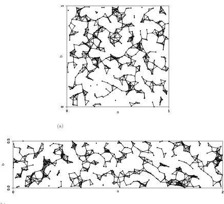
(a/b)→1. In this sense we can say that the RRG is a generalization of the RGG. In Fig. 1
we illustrate an RGG and an RRG constructed with the same number of nodes and edges.
An interesting question is what happens at the other extreme, when a → ∞. In this
case we have that b → 0, which means that the n points are uniformly and independently
distributed on the straight line. Let us now consider a disk of radiusr >0centered at each of
these points and let us connect every point to the other points which lie inside its disk. Thus,
the resulting graph resembles a one-dimensional RGG, that is a graph created by placing
the n points uniformly and independently on the interval [0,1] and then connecting pairs
of nodes if they are at a (Euclidean) distance smaller than or equal to a certain connection
(a)
a
b
0 1
0
1
(b)
a
b
0 2
0.0
[image:5.595.72.509.105.503.2]0.5
Figure 1. Illustration of two random rectangular graphs with a = 1 (top), which corresponds to
a random geometric graph on a unit square and with a = 2 (b= 0.5) (bottom). Both graphs are built with 500 nodes and 1750 edges.
III. TOPOLOGICAL PROPERTIES OF RRGS
A. Average degree
We start the study of the topological properties of RRGs by considering an analytical
expression for the average degree ¯k. We remind that the degree of a node is the number
of edges connected to it. The average degree is a property not only interesting by itself
topological parameters of RRGs.
To start with, let us consider that for a given node, there are n−1 nodes distributed in
the rest of the rectangle. Define Ap to be the area within the radius r of a point p which
lies within the rectangle. Since the nodes are uniformly and independently distributed, the
expected node degree of a nodevi isE(ki) = (n−1)Ai/(ab), whereAi is taken for the point
where nodeviis located. This is because dividing the nodes between the area within distance
r and the rest of the rectangle gives rise to the Binomial distribution Bin(n−1, Ai/(ab)).
Averaging this over all possible node locations (i.e., the points in the rectangle) gives
Ek¯=
´
p{(n−1)Ap/(ab)}
ab =
(n−1)´
pAp
(ab)2 . (1)
Letf(a, b, r)be the area within radius rof a point which lies in the rectangle, integrated
over all points, i.e., f(a, b, r) = ´
pAp. Based on preliminary computational results (not
shown) obtained for the average degree we consider here the following three regions: 0 ≤
r ≤b, b ≤r ≤a and a ≤r ≤√a2+b2, recalling that a
≥b. We call these cases 1, 2 and
3, respectively. Thus, the function f(a, b, r) takes different forms fi for each case i. This
means that we can write
E¯k= (n−1)fi
(ab)2 , (2)
with
fi=
f1 0≤r≤b,
f2 b≤r≤a,
f3 a≤r≤
√
a2+b2,
(3)
and our task is now to find the analytical expressions forfi.
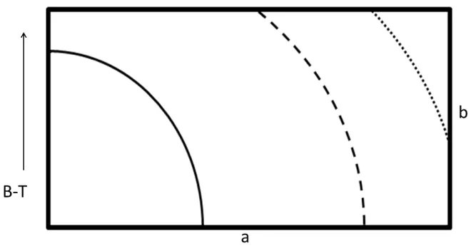
We consider the rectangle in Fig. 2, which shows 3 quarter circles of different radii (each
corresponding to one of the three cases) as they intersect the interior of the rectangle. We
consider only quarter circles instead of circles, then quadruple the result at the end. For
each of these quarter circles, we divide them into vertical rectangular strips of width ∆x
which will approximate the areas of the intersection between the quarter circles and the
full rectangle; this will become exact in the limit as ∆x → 0. We now consider several
Figure 2. Illustration of three different quarter circles in the rectangle corresponding to 0≤r ≤b (solid line), b≤ r ≤ a (broken line) and a ≤ r ≤ √a2+b2 (dotted line). The direction used for displacing the circles is represented as bottom-top (B-T) with an arrow in the graphic.
First, the strips may approximate an area which is not rectangular, which occurs when
the height of the strip is smaller than the height b of the rectangle. For a strip of distance
xfrom the left of the rectangle, this corresponds to0≤x≤r for the smaller quarter circle
(case 1), √r2−b2 ≤ x ≤ r for the medium quarter circle (case 2), and √r2−b2 ≤x ≤ a
for the largest quarter circle (case 3). Setting p = min(a, r), q = min(b, r), we have
p
r2−q2 ≤x≤p.
Since we need to integrate these areas over all possible quarter circles, given a fixed
radius, we wish to know how we can translate the quarter circle in the figure and preserve
a particular strip. That is, for a particular strip of distance xfrom the left of the rectangle,
we may find a corresponding strip on the other quarter circles of the same radius. Since we
have a rectangular strip of width ∆x, height √r2
−x2, and distance x from the center of
the (quarter) circle, we may find this strip in any of the(a−x−∆x)positions horizontally,
and(b−√r2−x2)vertically. Thus, we can use integration to find the total area of all these
strips by multiplying (a−x−∆x)(b−√r2
−x2)by the area of the strip√r2
taking the limit to obtain
I1 =
ˆ p √
r2−q2
(a−x)(b−√r2−x2)√r2−x2dx
=
ˆ p √
r2−q2
(a−x)(b√r2 −x2
−(r2 −x2
))dx. (4)
Secondly, we note that if these strips are translated far enough in the bottom-top (B-T)
direction, they become truncated by the top of the rectangle. For a particular truncated
strip, we may still find a corresponding strip in any of the (a−x−∆x) positions horizontally,
and the truncated height t of a strip may be any value between 0 and the full height of the
strip. Thus, integrating gives
I2=
ˆ p √
r2−q2
(a−x)
ˆ
√
r2−x2
0
t dt dx
=
ˆ p √
r2−q2
1
2(a−x)(r 2
−x2
)dx. (5)
Alternatively, we may have √r2
−b2 > b, in which case the rectangular strip is exact
and of height b. In this case, the only contribution is from the truncated strips. We note
that this applies for0≤x≤pr2
−q2 by a similar argument as before, and we integrate as
follows
I3=
ˆ √r2−q2
0
(a−x)
ˆ b
0
t dt dx
=
ˆ √r2−q2
0
1
2(a−x)b 2
dx. (6)
Thus, we have the expression for f as four times the sum of the above integrals
f = 4(I1+I2+I3)
=
ˆ √r2−q2
0
2(a−x)b2
dx+
ˆ p √
r2−q2
(a−x)(4b√r2 −x2
−2(r2 −x2
))dx, (7)
f =
0≤r≤b πr2ab −4
3(a+b)r 3+ 1
2r 4,
b≤r ≤a −4
3ar 3
−r2b2+ 1 6b
4+a(4 3r
2+ 2 3b
2)√r2−b2
+2r2abarcsin(b r),
a≤r≤√a2+b2
−r2(a2+b2) + 1 6(a
4+b4) −1
2r 4
+b(4 3r
2+ 2 3a
2)√r2
−a2+a(4 3r
2+ 2 3b
2)√r2 −b2
−2abr2(arccos(b
r)−arcsin( a r)).
(8)
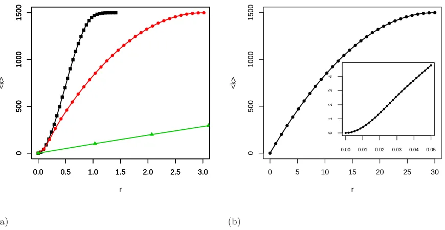
Now we evaluate computationally how good the expression for the average degree of the
RRGs is. In Fig. 3(a) we plot the values of the average degree observed for RRGs with
three different values of the rectangle side length. These observed values (represented by
solid squares, circles and triangles) are the average of 100 random realizations of RRGs with
n= 1,500nodes. The solid lines represent the expected values according to the expressions
(8). The Pearson correlation coefficients for the linear regression between the observed and
expected values are larger than 0.9999 in the three cases. We enlarge the region of small
radii for the case a= 30(see Fig. 3 (b)) where it can be seen that it is a perfect fit also for
this region with Pearson correlation coefficient as good as for the general case.
B. Connectivity
In this section we are interested in determining the connection radius for specific values
ofn, i.e.,r(n), which guarantees that the RRGΓ (n, r(n))is asymptotically connected with
probability one. For the RGG, Penrose [31] proved that ifMn is the maximum length of an
edge in the graph, then the probability that nπM2
n−logn≤α for a given α∈Ris
lim
n→∞P
nπM2
n−logn≤α
= exp (−exp (−α)). (9)
In 2DMn =r , such that we have for the RGG
lim
n→∞P
nπr2
−logn≤α
= exp (−exp (−α)). (10)
This means that for α → +∞ the RGG is almost surely connected when n → ∞, and
(a)
0.0 0.5 1.0 1.5 2.0 2.5 3.0
0
500
1000
1500
r
<k>
0.0 0.5 1.0 1.5 2.0 2.5 3.0
0
500
1000
1500
0.0 0.5 1.0 1.5 2.0 2.5 3.0
0
500
1000
1500
(b)
0 5 10 15 20 25 30
0
500
1000
1500
r
<k>
0.00 0.01 0.02 0.03 0.04 0.05
0
1
2
3
4
Figure 3. (color online) (a) Illustration of the fit between the observed (black squares (a= 1), red circles (a= 3), and green triangles (a= 30)) and expected (solid line) values of the average degree
for RRGs with different side lengths of the rectangle. (b) Wider range of radii fora= 30(zooming
for the small radii in the inset).
The term nπr2 is just the average degree k¯ in RGG (when no boundary effects are
considered). Thus we can write
lim
n→∞P
¯
k−logn≤α
= exp (−exp (−α)). (11)
In the previous section we have obtained an analytic expression for¯k in the RRG. Thus,
we can replace this in (11) and obtain an analogous expression for the RRG. That is, for a
RRG we have that
lim
n→∞P
(n−1)fi
(ab)2 −logn≤α
= exp (−exp (−α)), (12)
where fi is given by (8).
Because the parameterαis unknown and it depends on the specific RRG considered, we
[image:10.595.74.509.134.359.2]exp
−exp
−
(n−1)fi
(ab)2 −logn
≤exp (−exp (−α)). (13)
Now we consider the computational evaluation of the connectivity of RRGs with 1,500
nodes as a function of the connection radius and the rectangle side length. We start by
analyzing the goodness of the upper bound that we have found for the probability of a RRG
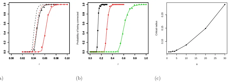
to be connected (see (13)). In Fig. 4(a) we illustrate the plot of the probability of being
connected versus the connection radius for graphs embedded into rectangles of side length
a= 1(black circles) anda= 10(red circles). The solid circles represent the average values of
100 random realizations for these graphs. The values corresponding to the upper bound are
plotted as broken lines. As can be seen, both the observed and the upper bound follow the
same distribution and the upper bound is relatively close to the average observed values. In
Fig. 4(b) we illustrate the change in the probability that the RRG is connected as a function
of the connection radius, i.e., the minimum radius needed to make the network connected,
for three different values of a. As the square is elongated the critical radius increases with
the value of a. For instance, for a= 1 the critical radius is about 0.2, and for a = 10 it is
about 0.9. Then, for a= 1, α ≥185.3for the RRG to be connected. This value increases
up to α≥750.8for a= 5 and toα≥3813.8for a= 10. The main reason for this increase
in the critical radius is that as we elongate the rectangle the points have to cover a longer
region and consequently their separation increases. As a consequence, we need to increase
the connection radius in order to guarantee the connectivity of the network. In other words,
increasing the value ofanecessarily implies having to increase the connection radius to make
the network connected. The global increase of the critical radius with the side length of the
rectangle is given in Fig. 4 (c).
C. Degree distribution
In the RRG the n nodes are distributed uniformly and independently on the unit
rect-angle. Then, the degree distribution can be easily estimated by considering the probability
density function of having a node i of degree ki given that there are n−1 other nodes
uniformly distributed in the unit rectangle (see for instance [32]). This gives rise to the
(a)
0.00 0.02 0.04 0.06 0.08 0.10
0.0 0.2 0.4 0.6 0.8 1.0 r
Probability of being connected
0.00 0.02 0.04 0.06 0.08 0.10
0.0 0.2 0.4 0.6 0.8 1.0
0.00 0.02 0.04 0.06 0.08 0.10
0.0 0.2 0.4 0.6 0.8 1.0
0.00 0.02 0.04 0.06 0.08 0.10
0.0 0.2 0.4 0.6 0.8 1.0
0.00 0.02 0.04 0.06 0.08 0.10
0.0 0.2 0.4 0.6 0.8 1.0
0.00 0.02 0.04 0.06 0.08 0.10
0.0 0.2 0.4 0.6 0.8 1.0 (b)
0.0 0.2 0.4 0.6 0.8 1.0
0.0 0.2 0.4 0.6 0.8 1.0 r
Probability of being connected
0.0 0.2 0.4 0.6 0.8 1.0
0.0 0.2 0.4 0.6 0.8 1.0
0.0 0.2 0.4 0.6 0.8 1.0
0.0 0.2 0.4 0.6 0.8 1.0
0.0 0.2 0.4 0.6 0.8 1.0
0.0 0.2 0.4 0.6 0.8 1.0
0.0 0.2 0.4 0.6 0.8 1.0
0.0 0.2 0.4 0.6 0.8 1.0
0.0 0.2 0.4 0.6 0.8 1.0
0.0 0.2 0.4 0.6 0.8 1.0 (c)
0 5 10 15 20 25 30
[image:12.595.78.511.124.281.2]0.10 0.15 0.20 a Cr itical r adius
Figure 4. Dependence of the probability of being connected with the connection radius in RRGs.
a) Illustration of the goodness of the bound (13) for two RRGs with a = 1 (black curves), and
a = 5 (red curves). The observed values for RRGs with 1,500 nodes averaged over 100 random
realizations are illustrated as solid circles and the values obtained by the theoretical bound are
given by broken lines. (b) Observed values of the probability of being connected for RRGs with
1,500 nodes averaged over 100 random realizations and three different rectangle side lengthsa= 1
(black squares), a = 5 (red circles), and a = 10 (green triangles). (c) Variation of the radius for which the RRG is connected (critical radius) with the rectangle side length for RRGs with 1,500
nodes and 11,250 edges.
p(k) =
n
k
pk(1−p)
n−k. (14)
Whenn→ ∞ andpis sufficiently small, this binomial distribution approaches very well
a Poisson distribution of the form
p(k)≃ k¯
kexp −¯k
k! . (15)
As we have previously obtained an analytic expression for the average degree ¯k we can
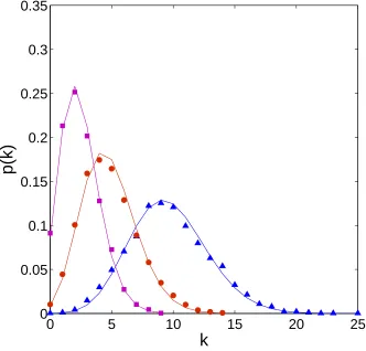
easily compute the degree distribution for RRGs. We select RRGs with 5,000 nodes and
radius of connection equal to 0.025. Then, we obtain the degree distribution for different
values of the rectangle side length and take the average of 100 random realizations. In Fig. 5
we also plot the expected distribution using the equation (15) in which we have plugged the
0
5
10
15
20
25
0
0.05
0.1
0.15
0.2
0.25
0.3
0.35
k
[image:13.595.132.464.111.429.2]p(k)
Figure 5. Degree distribution of RRGs withn= 5,000, connection radius r= 0.025, and rectangle side lengths a = 1 (triangles), a = 50 (circles), a = 100 (squares). The solid figures (triangles,
circles and squares) correspond to the average of 100 random realizations for the given network.
The solid lines correspond to the shape of the Poisson distribution (15) with the corresponding
average degree obtained from eq. (8).
of the side length of the rectangle, the RRG displays Poisson degree distributions. That is,
the elongation of the rectangle does not affect the shape of the degree distribution of the
nodes.
D. Average shortest path distance
Let Γ = (V, E) be a simple connected graph. A path of length k in Γ is a set of nodes
i1, i2, . . . , ik, ik+1 such that for all 1 ≤ l ≤ k, (il, il+1) ∈ E with no repeated nodes. The
shortest path connecting these nodes. We will write d(u, v)to denote the distance between
u and v. Here we will define, as is usual in network theory, the average path length to be
the following quantity:
hli= 2
n(n−1)
X
u<v
d(u, v). (16)
The diameter of the graph is defined as the maximum of all the shortest path lengths in
the graph, i.e., D = maxu,vd(u, v).We consider here an upper bound for the average path
length. Then, we start by considering that the n points are distributed homogeneously in
the rectangle of sides a andb=a−1 in such a way that the points are equally spaced in the
rectangle and are separated by a Euclidean distance r. In this case, the point which is the
farthest from the rest of the n−1points in the rectangle is one at any of the four corners of
the rectangle. Let us designate this point asi. If the average path length of this node ishlii,
it is straightforward to realize thathli ≤ hlii, and we will have the desired upper bound. It
is easy to see that the largest chain of connected points is realized along the main diagonal
of the rectangle. Thus, the longest distances involving the node i are those connecting it
with the other nodesj along the main diagonal of the rectangle. Let us designate the length
of the main diagonal is c. Then, there are D = c
r connected nodes in this line. Let us now
consider hlii based only on those j nodes along the main diagonal of the rectangle (notice
that this is an upper bound for hlii). That is
X
j∈diag
dij = 1 + 2 +· · ·+D =
D(D+ 1)
2 .
Consequently,
hlii ≤
D(D+ 1)
2D =
D+ 1
2 .
Because, hli ≤ hlii, we have
hli ≤ hlii ≤
D+ 1
2 .
It is easy to note that D < a
r +
1
ar. That is, the length of the diagonal is smaller than
the sum of the length of the two sides of the rectangle (in terms of number of nodes), which
are a
r and
b
r =
1
hli ≤ hlii ≤
D+ 1
2 ≤
a
r +
1
ar+ 1
2 =
a2+ar+ 1
2ar . (17)
An important consequence of this bound is that it allows us to find the asymptotic
behavior of the average path length as the rectangle becomes more elongated. That is,
if we fix the connection radius we can see that lima→∞hli = ∞. In other words, as the
rectangle becomes more elongated the RRG becomes a large-world with a very large average
shortest path distance. As a→ ∞, the connection radius rhas to be increased to keep the
connectivity of the RRG. Thus, the infinite growth of the path length is not observed in
practice due to the connectivity constraints imposed by the connection radius. Our further
calculations show that the average path length is of the same order of magnitude as the
right-hand side of eq. (17), which means that we can write it as:
hli ∼ a
2
+ar+ 1
2ar . (18)
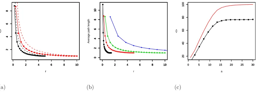
We now study computationally RRGs with 1,500 nodes. For every value ofa we report
the average of 100 random realizations. First, we analyze the goodness of the upper bound
found here for the average path length. In Fig. 6(a) we illustrate the variation of hli with
the connection radius for two different values of a, namely a = 5 and a = 10. In the same
plot we illustrate the values of the upper bound obtained with the expression (17), where
it can be seen that the upper bound is very close to the average shortest path obtained
for these RRGs. Particularly, for large values of r the observed values are almost identical
to those of the upper bound. As observed in Fig. 6(b) the average path length not only
changes with the variation of the connection radius but also with the rectangle side length.
This is already expected from the eq. (18) where it can be seen that asa→ ∞the average
path length also grows to infinity for fixed r (see observation at the end of the previous
paragraph).
These results agree with our intuition that as we elongate the rectangle there are nodes
which are farther apart from each other and as a result the average path length of the whole
graph increases. For a better analysis of this relation we plotted the results of the average
path length for 100 random realizations of the previously mentioned RRGs versus a, with
m= 11,250edges, in Fig. 6(c). We also plot here the upper bound (17). It can be seen that
(a)
0 2 4 6 8 10
2 4 6 8 r <l>
0 2 4 6 8 10
2
4
6
8
0 2 4 6 8 10
2
4
6
8
r
0 2 4 6 8 10
2
4
6
8
(b)
0 2 4 6 8 10
0 2 4 6 8 10 r A v er
age path length
0 2 4 6 8 10
0 2 4 6 8 10
0 2 4 6 8 10
0 2 4 6 8 10
0 2 4 6 8 10
0 2 4 6 8 10
0 2 4 6 8 10
0 2 4 6 8 10 (c)
0 5 10 15 20 25 30
20 40 60 80 100 a <l>
0 5 10 15 20 25 30
20
40
60
80
100
Figure 6. (a) Plot of the average path length for RRGs with n = 1,500 nodes with different
connection radii fora= 5(black squares) and fora= 10(red squares). The solid squares represent the average of hli for 100 random realizations (lines connecting the squares are used to guide the eye). The dotted lines represent the upper bounds (17) forhliin RRGs for the corresponding values of a. (b) Change of the average path length versus radius for networks with n= 1,500 nodes for different values of a: black squares (a = 1), red circles (a = 5), green triangle (a = 10), blue
rhombus (a = 30). (c) Illustration of the upper bound (solid line) for the average path length as a function of a for a network with the same size as before and connection radii that guarantees
m= 11,250edges for a given value of a.
is very flat. In this region we have thata→ ∞, which corresponds to a good approximation
of a one-dimensional RGG. Fora= 1it is known that the average path length depends only
on the inverse of the radius, hlei = Θ(1/r). The actual radius used for the plot in Fig. 7
(c) is r = 0.0578, which gives an estimate of the average path length of 17.3, which is not
too far from the observed value in the plot for a = 1. In the case of a = 30 we are in the presence of a very elongated rectangle, which is very similar to a one-dimensional RGG. A
crude estimate of the average path length in this case would behlei=n/hki, which in the
current case will give hlei ≈100, which is relatively close to the observed value ofhli ≈ 75
[image:16.595.75.512.125.282.2]E. Clustering coefficient
One of the most important network parameters is the local clustering coefficient,usually
known as theWatts-Strogatz clustering coefficient,of a node i. This parameter is defined as
[10]:
Ci=
2ti
ki(ki−1)
, (19)
where ti is the number of triangles involving the node iandki is the degree of the node
i. Taking the mean of these values as ivaries among the nodes in Γ, one gets the average
clustering coefficient of the network: hCi= 1
n
Pn
i=1Ci.
The average clustering coefficient of a RGG has been obtained by Dall and Christensen
[17] for r2 = logn+α
nπ when n → ∞ and α → ∞, where α ∈ R is a constant for a given
number of nodes (see Section B. Connectivity):
hCdi=
1−Hd(1) d even
3
2Hd(1/2) d odd,
(20)
where d is the dimension of the hypercube in which the nodes are embedded and
Hd(x) =
1 √π
d/2
X
i=x
Γ (i) Γ i+ 1
2
3 4
i+12
, (21)
where Γ (i) is the Gamma function. Thus, for d= 2 , hC2i = 1−
3√3
4π ≈0.5865 and for
d= 1, hC1i= 3/4 = 0.75.
Here, however, we are interested in an expression that accounts for the variations of the
clustering coefficient with both the connection radius and the rectangle side length. Our
strategy is similar to the one used in [17]. That is, let i and j be two connected nodes in
a RRG, which are separated at a Euclidean distance δ from each other. Let us draw two
circles of radius r centered respectively at i and j. Let δ ≤ r such that the two nodes are
connected. Then, because δ < 2r the two circles overlap. Because i and j are connected,
any point in the area formed by the overlap of the two circles will form a triangle with the
nodes i andj . In addition, any node inside the two circles which is not in the overlapping
area forms a path of length two with the nodes i and j . Thus if we quantify the ratio of
triangles to open triads in which the nodesiandj take place, i.e., the clustering coefficient.
This ratio is given by
hCi=
2r2arccos
δ
2r
− 12δ√4r2 −δ2
πr2 . (22)
At this point we only need an estimation of the length δ between two connected nodes
in a RRG. We use here a simple approach based on the following intuition. Let us start by
considering nnodes in a square in such a way that they form a regular square lattice. Then,
δis proportional to the length of the side of the rectangle adivided by the number of circles
along this side. As we have a square, the number of points along the side of length ais the
same as that for the other side. Consequently, δ ∼ n−1/2
. If we elongate the rectangle to
a → ∞, which resembles a straight line, we will have that the separation between the two
points is just the length of the straight line divided by the number of nodes, δ∼an−1. For
a general rectangle the separation between two points in a line along the edge side of length
a is given by δ∼ an−γ, where γ ∼ a(a+b)−1
. Notice that when a = 1 (b = 1) we have
δ∼n−1/2 and when a
→ ∞ (b →0) we have δ∼an−1. We remind the reader that here we
consider only the caseb= a−1.
Plugging δ ∼ an−γ, with γ ∼ a(a+b)−1
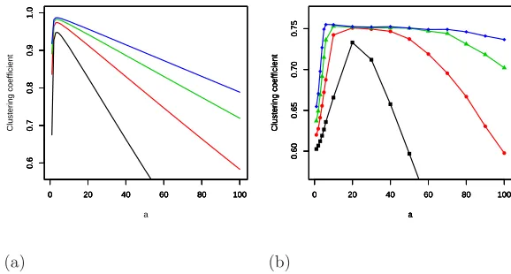
into (22) we obtain some surprising results.
In Fig. 7(a) we illustrate the dependence of hCi with a for different radii based on the
equation (22) with the estimated value ofδ given before. Notably, the clustering coefficient
is predicted to change non-monotonically with the rectangle side length. Instead, for small
values of a the clustering coefficient is predicted to increase to a maximum value and after
it the clustering decreases linearly. In addition, according to this model, as the connection
radius increases the clustering coefficient is expected to increase for the same value of a. In
closing, the largest value of the clustering is expected for certain specific value of a and a
relatively large connection radius.
In order to verify these findings we compute the average clustering coefficient of RRGs
with n = 1,500 and the same connection radii used in the simulations with the analytical
formulas. The results of the variation of the clustering with the rectangle side length are
illustrated in Fig. 7(b). As can be seen the clustering increases up to a maximum, whose
lo-cation depends on the connection radius, and then decays with the increase of the elongation
our previous reasoning, but we very well captured the behavior of the clustering of having a
non-monotonic change witha. Also, these experiments show that the increase of the
connec-tion radius increases the average clustering coefficient as predicted by our analytical results.
As can be seen in Fig. 7 (b) for a= 1and small radius the average clustering coefficient is
hCi ≈0.61,which is very close to the expected value for the 2-dimensional RGG according
to [17]. When a = 30and the radius is relatively large, the average clustering coefficient is
hCi ≈ 0.75, which coincides with the exact value expected for the one-dimensional RGG
according to [17]. Consequently, the RRG generalizes the values of the clustering coefficient
of both, the one- and two-dimensional RGG, fora= 1anda→ ∞, respectively. In addition,
it provides a series of intermediate values of the clustering coefficient for intermediate values
of the side length of the rectangle.
(a)
0 20 40 60 80 100
0.6 0.7 0.8 0.9 1.0 a Cluster ing coefficient
0 20 40 60 80 100
0.6
0.7
0.8
0.9
1.0
0 20 40 60 80 100
0.6
0.7
0.8
0.9
1.0
0 20 40 60 80 100
0.6 0.7 0.8 0.9 1.0 (b)
0 20 40 60 80 100
0.60 0.65 0.70 0.75 a Cluster ing coefficient
0 20 40 60 80 100
0.60 0.65 0.70 0.75 a Cluster ing coefficient
0 20 40 60 80 100
0.60 0.65 0.70 0.75 a Cluster ing coefficient
0 20 40 60 80 100
[image:19.595.145.434.364.519.2]0.60 0.65 0.70 0.75 a Cluster ing coefficient
Figure 7. Illustration of the dependence of the clustering coefficient with the rectangle side length for
different connection radii: r= 0.05(black),r= 0.1(red),r= 0.15(green)r= 0.20(blue). In plot (a) we show the analytical results and in plot (b) the observed ones. Both results are obtained for
RRG with 1,500 nodes and for the observed ones we averaged the results of 100 random realizations.
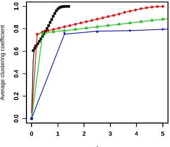
We now further explore the relation between the radius r and the clustering for RRGs
with different side lengths. We consider graphs with n = 1,500 nodes and a = 1,5,10,30.
As the radius increases the graph is becoming more and more dense, which makes that the
clustering coefficient is characterized by an abrupt increase at the beginning of the plot and
then a linear increase until the value of hCi= 1is reached for the complete graph (see Fig.
0 1 2 3 4 5
0.0
0.2
0.4
0.6
0.8
1.0
r
A
v
er
age cluster
ing coefficient
0 1 2 3 4 5
0.0
0.2
0.4
0.6
0.8
1.0
0 1 2 3 4 5
0.0
0.2
0.4
0.6
0.8
1.0
0 1 2 3 4 5
0.0
0.2
0.4
0.6
0.8
1.0
Figure 8. (color online) Variation of the average path length with the radius for RRGs with 1,500
nodes anda= 1,5,10,30. Every point is the average of 100 random realizations.
6 CONCLUSIONS AND FUTURE OUTLOOK
We have introduced here a generalization of the RGG in which we embed the points into
a unit rectangle instead of on a unit square. We consider a rectangle with sides of lengths
aandb = 1/a, such that as whena= 1we have the particular case of the classical random
geometric graph embedded in a unit square. Also, when a→ ∞ we have a very elongated
rectangle which resembles a one-dimensional RGG. We have provided computational and
analytical evidence that reaffirm the fact that the topological properties of the RRG differ
significantly from those of the RGG. In this respect we have obtained analytical expressions
or bounds for the average degree, degree distribution, connectivity, average path length and
the clustering coefficient of RRGs. In general, these properties depend on the connection
radius as well as on the rectangle side length. Most of the dependencies found here for these
properties in terms of the rectangle side length are monotonic. The only exception is the
clustering coefficient. This index first increases up to a critical value of a which depends
on the connection radius, and then decays linearly with the increased elongation of the
rectangle.
The introduction of the RRGs opens new possibilities for studying spatially embedded
random graphs. For instance, the study of dynamical processes taking place on the nodes and
[image:20.595.208.375.132.276.2]dynamics on the RRGs. On the other hand, the analysis of rectangular proximity graphs,
such as the rectangular Gabriel graphs and random rectangular neighborhood graphs is
also interesting for many of the practical applications of these graphs as mentioned in the
Introduction. The generalization of the RRG model to higher dimensions is also of both
theoretical and practical interest. In closing, the current work is expected to open new
horizons for the study of random spatial graphs and its applications in physics and beyond.
IV. ACKNOWLEDGMENT
EE thanks the Royal Society for a Wolfson Research Merit Award. MS thanks Weir
Advanced Research Centre at Strathclyde and EPRSC for partial financial support of his
work. We thank the two anonymous referees for valuable suggestions that helped to improve
this paper.
[1] E. Estrada,Graphs and Networks, inMathematical Tools for Physicists, edited by M. Grinfeld,
(John Wiley & Sons, 2014).
[2] G. Berkolaiko, R. Carlson, S. A. Fulling, and P. Kuchment,Quantum Graphs and their
Appli-cations, (AMS, 2006).
[3] E. Estrada,The Structure of Complex Networks: Theory and Applications, (Oxford University
Press, 2011).
[4] M. E. J. Newman, SIAM Rev.45, 167 (2003).
[5] L. d. F. Costa, O. Oliveira, G. Travieso, F. A. Rodrigues, P. Villas Boas, L. Antiqueira, M.
Viana, and L. Correa Rocha, Adv. Phys. 60, 329 (2011).
[6] M. J. E. Newman, Preprint arXiv:cond-mat/0202208 (2002).
[7] B. Bollobás, Random Graphs, (Academic Press, New York, 1985).
[8] P. Erdös and A. Rényi,On the evolution of random graphs, Selected Papers of Alfréd Rényi,
Vol. 2, 482-525 (1976).
[9] A. L. Barabási and R. Albert, Science286, 509-512 (1999).
[10] D. J. Watts and S. H. Strogatz, Nature393, 440-442 (1998).
[12] D. Urban and T. Keitt, Ecology, 82, 1205 (2001).
[13] A. Perna, S. Valverde, J. Gautrais, C. Jost, R. Solé, P. Kuntz and G. Theraulaz, Physica A
387, 6235-6244 (2008).
[14] J. Buhl, J. Gautrais, R.V. Solé, P. Kuntz, S. Valverde, J.L. Deneubourg, and G. Theraulaz,
Eur. Phys. J. B42, 123 (2004).
[15] E. Santiago, J. X. Velasco-Hernández, and M. Romero-Salcedo, Exp. Syst. Appl.41, 811-820,
(2014).
[16] M. Penrose, Random geometric graphs (Oxford University Press, 2003).
[17] J. Dall, and M. Christensen, Phys. Rev. E66, 016121 (2002).
[18] P. Gupta and P.R. Kumar,Critical Power for asymptotic connectivity in wireless networks, in
Stochastic analysis, control, optimization and applications (Birkhäuser Boston, 1999).
[19] G. J. Pottie and W. J. Kaiser, Comm. ACM 43, 51-58, 5 (2000).
[20] D. Estrin, R. Govindan, J. Heidemann and S. Kumar, Next century challenges: Scalable
co-ordination in sensor networks, in Proceedings of the ACM/IEEE International Conference on
Mobile Computing and Networking (Seattle, Washington, USA, August 1999), p. 263-270.
[21] E. N. Gilbert, Ann. Math. Stat. 30, 1141-1144 (1959) .
[22] P. Wang and M. C. González, Phil. Trans. Royal Soc. A: Math., Phys. Eng. Sci. 367.1901,
3321-3329 (2009).
[23] A. Díaz-Guilera, J. Gómez-Gardeñes, Y. Moreno, and M. Nekovee, Int. J. Bif. Chaos19, 687
(2009).
[24] M. Nekovee, New J. Phys.9, 189 (2007).
[25] V. Isham, J. Kaczmarska, and M. Nekovee, Phys. Rev. E83,046128 (2011).
[26] Z. Toroczkai, and H. Guclu, Physica A378, 68-75 (2007).
[27] D. Watanabe, A study on analyzing the grid road network: patterns using relative
neighbor-hood graph, The Ninth International Symposium on Operations Research and Its Applications
(ISORA’10), Chengdu-Jiuzhaigou, China, ORSC & APORC. (2010).
[28] [3] M. Desai and D. Manjunath, Comm. Lett.6, 437-439 (2002).
[29] C.H. Foh, G. Liu, B. S. Lee, B. C. Seet, K. J. Wong and C.P. Fu, Comm. Lett.9, 31-33 (2005).
[30] E. Godehardt and J. Jaworski, Rand. Struct. Algorith.9, 137-161 (1996).
[31] M. D. Penrose, Ann. Appl. Prob.7, 340-361 (1997).
[33] G. Ercal, Small worlds and rapid mixing with a little more randomness on random geometric