Robust multi-disciplinary design and optimisation of a reusable launch vehicle

Robust Multi-disciplinary Design and Optimisation of

a Reusable Launch Vehicle

R. Wuilbercq

∗

, F. Pescetelli

∗

, A. Mogavero

∗

, E. Minisci

†

, R.E Brown

‡

Centre for Future Air-Space Transportation Technology,

University of Strathclyde, 75 Montrose Street, Glasgow G11XJ, United Kingdom

For various technical reasons, no fully reusable launch vehicle has ever been successfully constructed or operated. Nonetheless, a range of reusable hypersonic vehicles is currently being considered as a viable alternative to the expensive but more conventional expendable rocket systems that are currently being used to gain access to space. This paper presents a methodology that has been developed for the rapid and efficient preliminary design of such vehicles. The methodology that is presented uses multi-disciplinary design optimization coupled with an integrated set of reduced-order models to estimate the characteristics of the vehicle’s aero-thermodynamic, propulsion, thermal protection and internal system architecture, as well as to estimate its overall mass. In the present work, the methodology has been applied to the multi-disciplinary modelling and optimization of a reusable hybrid rocket- and ramjet-powered launch vehicle during both the ascent and re-entry phases of its mission.

I.

Introduction

F

uture trans-atmospheric vehicles will, by means of a complex hybrid propulsion system, accelerate up to orbital speed when still within the denser part of the terrestrial atmosphere. The high velocity of the vehicle, when combined with the high air density in the lower atmosphere, will expose it to a severe heating environment. By contrast, during atmospheric entry at very high speeds, the same vehicle will most likely follow an un-powered gliding trajectory during which deceleration to lower velocities will occur at high altitude where the density of the air is relatively low. Although it may be possible to design the vehicle so that the peak heating during descent may be somewhat lower than that experienced during ascent, the integrated heat load that will need to be dissipated or absorbed by the vehicle will not be very much different between the ascent and descent phases of the mission.

Despite the extreme heating conditions to which future space-access vehicles will be exposed, there will be strict emphasis on their full reusability in order to ameliorate their acquisition cost over multiple missions. Part of this strategy will indeed also be to limit costs by reducing the amount of maintenance and refurbishment that is required between flights. Designers will thus, in all likelihood, find themselves forced to employ a new approach to the design of the vehicle’s Thermal Protection System (TPS). This will almost certainly result in a switch from the classic insulated aircraft approach`a laSpace Shuttle to the use of a combination of passive, semi-passive, and active TPS.1_{The resulting TPS will likely make use of both}

lightweight protective materials and a complex Active Cooling System (ACS) involving the re-circulation of a coolant under the most severely heated parts of the structural skin.

Nonetheless, sizing the TPS exclusively for the high-temperature conditions to which the vehicle might be exposed during its mission might not necessarily ensure that the vehicle will meet all of its performance requirements. For instance, future RLVs will be held at their spaceport for a short period of time between flights to fill their cryogenic propellant tanks and to perform maintenance tasks. During these ground-hold operations, the vehicle will be exposed to ambient ground-level temperature, as opposed to the very high temperatures that characterize their in-flight mission profile. Heat transfer from the atmosphere to the TPS

∗_{PhD Student, Student Member AIAA} †_Lecturer

will therefore occur at a much lower rate and the materials that cover the cryogenic tanks might then need to be sized to prevent the hazardous formation of ice on the outer surface of the vehicle prior to launch.

This new generation of hypersonic vehicles is also foreseen to make use of hypersonic air-breathing engines, in particular ramjets or scramjets, in order to achieve the performance required for practical attainment of a Single-Stage-To-Orbit (SSTO) capability. Indeed, supersonic combustion is widely accepted to be the most promising alternative to the use of conventional rocket engines in this context. Instead of carrying separate tanks for fuel and oxidizer during take-off, scramjet-powered vehicles will need only to carry the fuel, using atmospheric oxygen for combustion. While air-breathing propulsion systems are characterized by a much higher specific impulse Isp than rockets, scramjets are subject to strong engine-airframe coupling, adding

significant complexity to the design of the vehicle.

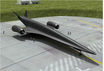
[image:2.612.95.521.287.579.2]

These various characteristics emphasize the need to generate and employ a very robust methodology in order to design and optimise future trans-atmospheric vehicle configurations efficiently at a system level. An integrated Robust Multi-disciplinary Design Optimisation (R-MDO) procedure must perforce be used and applied for both the ascent and re-entry phases of the vehicle trajectory in order to optimise concurrently the various subsystems to a point where the concept might become technically feasible. This article presents an attempt to define such a general R-MDO methodology. A prototype such methodology is then applied to study the sensitivity of a representative Reusable Launch Vehicle (RLV) configuration (see Fig. 1) to uncertainties and variability in some of its key design parameters.

Figure 1: The CFASTT-1 Reusable Launch Vehicle during ground-hold operations.

(Original graphic by Adrian Mann.)

II.

System Model

prototype for such a dedicated platform, called HyFlow, which is composed of several interrelated modules. These modules evaluate the aero-thermodynamic environment, optimise the performance of the propulsion system, size the protective shield, and finally predict the vehicle mass and trajectory while accounting for inherent uncertainty in the system parameters that are encapsulated within each of its constituent models. In the following sections of this article, each of these modules is described in more detail:

II.A. Earth model

The gravitational accelerationg is assumed to vary with altitude according to an inverse square law

g(h) =g0

h RE+h

2

(1)

wherehdenotes the altitude above mean sea level,RE= 6375 km is the mean radius of the Earth, andg0=

9.80665 m/s2 is the gravitational acceleration at sea level. The atmospheric characteristics (temperature, pressure, density and speed of sound) follow the 1976 US Standard Atmosphere model up to 1000 km. The effects of wind are not accounted for.

II.B. Trajectory Model

In the present work, the vehicle is modelled dynamically as a point with variable mass flying around a spherical, rotating earth. The translational motion of the vehicle along its trajectory is governed by the following set of differential equations:3

˙

h = vsinγ (2)

˙

v = FTcos−D

m −gsinγ+ω

2

E(RE+h) cosλ(sinγcosλ−cosγsinχsinλ) (3)

˙

γ = FTsin+L

mv cosµ−

g v −

v RE+h

cosγ+ 2ωEcosχcosλ

+ ω2E

_R

E+h v

cosλ(sinχsinγsinλ+ cosγcosλ) (4)

˙

χ = FTsin+L

mvcosγ sinµ−

_v

RE+h

cosγcosχtanλ

+ 2ωE(sinχcosλtanγ−sinλ)−ωE2

_R

E+h vcosγ

cosλsinγcosχ (5)

˙

λ =

_v

RE+h

cosγsinχ (6)

˙

θL =

_v

RE+h

_cosγcosχ

cosλ (7)

where v is the speed of the vehicle as measured in an Earth-centred reference frame (assumed to have a rotation rateωE = 7.2921×10−5 rad/s). In these equations,γindicates the flight path angle,χis the path

directional angle,µis the bank angle, andλandθLdenote respectively the latitude and the longitude of the

vehicle at timet. The mass of the vehicle ism,FT is the magnitude of the thrust produced by its engines,

andLandDdenote the aerodynamic lift and drag forces, respectively. The angle between the thrust vector and the velocity vector is, and finally ˙mf uelis the fuel mass flow rate. During ascent to orbit, the control

law for the vehicle governs the angle of attack α, the bank angle µ, and the thrust FT. Similarly, for the

re-entry phase of the mission, the control law governs the angle of attackα, and the bank angleµ. In both cases the vehicle is thus allowed to perform out-of-plane motions.

II.C. Aero-thermal Model

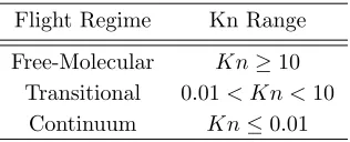
to free-molecular flow at high altitudes, passing through a transitional flow regime in between. The regime in which the vehicle is operating depends on a non-dimensional parameter called the Knudsen numberKn

which measures the relative importance of the particulate nature of the gas. The Knudsen number is formally defined as the ratio of the mean free path of the gas, denotedλgas, through which the vehicle is travelling to

an appropriate measure of the dimensions of the vehicle (e.g. the nose radius or mean aerodynamic chord, depending on context). The various flow regimes encountered by an RLV during its mission, as a function of the Knudsen number, are summarized in Table 1.

Flight Regime Kn Range

Free-Molecular Kn≥10

Transitional 0.01< Kn <10

[image:4.612.228.386.148.212.2]

Continuum Kn≤0.01

Table 1: Flight Regimes encountered by an RLV as a function of the Knudsen NumberKn.

II.C.1. Aero-thermodynamic Environment

The aero-thermodynamic module in HyFlow uses a combination of independent panel compression methods to predict the aero-thermodynamics of vehicles travelling at supersonic or hypersonic Mach numbers. The model automatically selects the appropriate method based on estimation of the local Knudsen number in conjunction with a topological feature detection technique to discriminate planar from non-planar regions of the flow geometry to switch from modified Newtonian theory to a tangent-wedge or tangent-cone approxima-tion where appropriate. When the estimated Knudsen number lies within the transiapproxima-tional regime, HyFlow use a bridging technique, defaulting to a simple sine-squared law in the absence of a better approximation, to interpolate between the predictions obtained from its free-molecular and continuum-flow models.

HyFlow accounts for viscous effects by calculating the trajectories of the surface streamlines, using these to determine the local Reynolds number and then integrating the skin friction coefficients for compressible turbulent or laminar flow over a flat plate. The Smart-Meador reference temperature method is used for both laminar and turbulent boundary layers.4 _{Temperature effects are included by using Sutherland’s viscosity}

law in order to account for the variation of viscosity with temperature, using standard temperature and pressure as the reference values.

HyFlow can evaluate the aero-thermal load at the surface of the vehicle using a technique that is based directly on the flat-plate reference temperature method that is used, as described above, to evaluate the skin friction coefficients. The well-known Reynolds analogy is used to obtain an estimate of the Stanton number,

St, and thus the local convective heating rate ˙qconv. Since the method based on the Reynolds analogy

and streamline tracing is inherently invalid at stagnation features within the flow, a mix of methods is employed in practice, making use of a modified version of the Fay-Riddell formula to calculate the convective heating rate for general three-dimensional stagnation features5 based on the estimation of the local radius of curvature.6 _{HyFlow can also be run in fully laminar, fully turbulent, or transitional modes. A simple}

prediction correlation, based on experimental data for sharp cones at zero angle of attack, and used by Bowcuttet al.7 _{in their study of hypersonic waveriders, is presently used to predict the onset of}

laminar-turbulent transition on the surface of the vehicle.

HyFlow is a panel-based implementation which uses an unstructured triangular mesh to describe the geometry of the vehicle being modelled. Piecewise constant surface properties are assumed across the area of each panel and the accuracy of the model thus increases as the number of triangular faces is increased. A moderately coarse mesh is usually employed in order to maintain a relatively good computational efficiency, particularly when using the model in optimization studies, but local mesh refinement can be applied judi-ciously in sensitive regions of the geometry, such as on highly curved surfaces and near stagnation features, to improve the overall accuracy of the predictions.8

II.D. Thermal Protection System Model

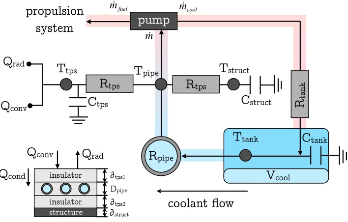
need for light weight and serviceability together with resistance to high temperatures will most likely require that the passive use of lightweight insulation materials be augmented, at least on the most exposed parts of the vehicle (e.g. the leading edge of the wing, and the nose region), by a complex Active Cooling System (ACS) involving the flow of a cryogen (possibly part of the vehicle propellant) through actively cooled surface panels. In this paper, it is assumed that the structural skin of the RLV is itself made of a thermally resilient material and thus that surface insulation is not required in those areas where the surface temperature does not exceed a predetermined threshold. In the process of sizing the TPS, the geometry of the vehicle is first partitioned into a number of self-consistent ‘thermal zones’: this task is performed automatically by the routines implemented within HyFlow’s thermal protection model. Within each of these zones, the convective heating profile on the panel that is most severely heated along the trajectory of the vehicle is used to size the thickness of the insulation layer, or the properties of the active cooling system that is required, as appropriate.

T

tps

Q

rad

Q

conv

R

tps

T

struct

T

pipe

coolant flow

C

tank

pump

R

tps

insulator

insulator

∂tps1

V

_cool

Q

conv

Q

rad

propulsion

system

_!

m

∂tps2

Dpipe

R

pipe

Q

cond

T

tank

C

struct

structure

R

tank !

mcool

!

m

_fuel

[image:5.612.130.484.230.456.2]

∂struct

C

tps

Figure 2: Conceptual thermal network for the Active Cooling System (ACS).

TPS Thermal Network

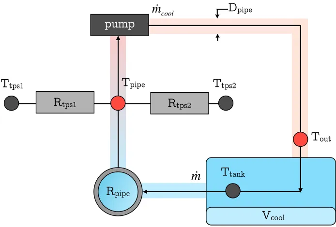
The schematic of a simplified active thermal management unit and its equivalent thermal network are depicted in Fig. 2. In the present model used within HyFlow, the conductivity of the feeder lines, through which the coolant flows, is neglected on the assumption that they would be made of a thin layer of highly conductive material to enhance the cooling of the most severely heated parts of the aircraft skin. Similarly, the TPS module presently assumes any Reusable Surface Insulation (RSI) to be attached directly to the underlying structural skin of the vehicle, as shown at the bottom left of Fig. 2.

The mass flow rate of cryogen (denoted ˙mcool and assumed here to be some of the liquid hydrogen

propellant) required to actively cool the vehicle can then be evaluated from the coolant mass flow rate (Eq. 8), which must perforce be designed in order to maintain the structural skin of the vehicle below its prescribed threshold temperature:

˙

mcool=ρcoolApipeUcool (8)

where ρcool is the density of the cryogenic fuel, Apipe is the cross-sectional area of the feeder lines, and Ucool is the velocity of the pumped coolant flowing through the piping system. Any effects due to boiling

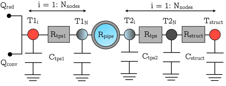
the system is taken to represent the average temperature of the associated sub-volume of the system (see Fig. 3). Similarly, the (thermal) capacitance assigned to any node is computed from the material properties evaluated at the temperature of the node and is assumed to be concentrated at the nodal centre of the sub-volume.9

C

tps2

C

struct

C

tps1

T1

i

Q

rad

Q

conv

R

tps

T

struct

R

tps1

R

pipe

R

struct

i = 1: N

nodes

T1

N

T2

i

T2

N

[image:6.612.120.493.114.256.2]

i = 1: N

nodes

Figure 3: Schematic of the TPS thermal network.

The nodeT1i in Fig. 3, is assumed to be directly exposed to the external flow; the temperature here is thus

dependent on the convective heating from the flow at the surface of the vehicle and the radiative cooling of the surface of the vehicle during its passage through the terrestrial atmosphere. These effects are modelled as external power sources to the thermal network as

Qconv= ˙qconvAi (9)

and

Qrad=tpsσAiT14 (10)

whereAi represents the surface area of the thermal zone being sized, ˙qconv(t) represents the convective heat

transfer profile experienced by the thermal zone along the vehicle trajectory, andtps andσare, respectively,

the emissivity of the surface coating and the Stefan-Boltzmann constant. The various sub-volumes that comprise the entire TPS can be modelled by defining an arbitrary number of material nodes,Nnodes, each

of which are assumed to have a (thermal) capacitance

Ci=ρiciVi (11)

where the density and specific heat of the TPS material (or fluid) are, respectively,ρi andci, andVi is the

volume of material available to absorb the thermal load. Each layer of TPS is also assumed to be made out of a material whose conductivity is ki. As pictured in Fig. 3, in the present study, two protective layers, of

thicknessδ1 andδ2 respectively, have been located on either side of the ACS feeder lines. The last node of

the first layer and the first node of the second layer of TPS are indeed considered to be in direct contact with the ACS feeder lines over an equivalent area that here is simply assumed to be equal to the surface area

Ai of the thermal zone under consideration. Finally, the set of feeder lines underneath the first TPS layer is

modelled as an equivalent convective resistance

Rpipe= 1/(hf uelAi) (12)

where hf uel is the convective heat transfer coefficient, thus allowing the cooling of the TPS by the forced

convection of the pumped cryogen within the pipe to be accounted for. An appropriate empirical formula,9

depending on the nature of the flow (i.e. on whether it is laminar or turbulent), is used to obtain the forced convective heat transfer coefficient of the coolant. Finally, by application of a thermal energy balance, where the energy flowing into each node must equal the sum of the heat flowing out together with the amount of thermal energy stored at each node, the time evolution of the nodal temperatures within the prescribed ACS scheme can be obtained. After selection of the various materials to be employed within the TPS, a combination of parameters such as the mass flow rate ˙mf uel, the pipe hydraulic diameter Dpipe, and the

thicknesses of the RSI layersδi must perforce be designed to prevent the structural temperature from rising

Tank Thermal Network

C

tank

V

cool

T

tank

R

tank

!

[image:7.612.152.434.72.317.2]

m

_cool

Figure 4: Thermal energy balance at the cryogenic tank.

It is assumed that, during the ascent of the vehicle, any cryogen that is used within the ACS will be sent directly to the propulsion system where it will be mixed with the main fuel supply and fed into the engines. No other provision thus has to be made to store or dissipate the energy that is extracted from the TPS during this phase of the mission. During re-entry, the situation is more difficult, since some means must be found to absorb or dissipate within the system the energy that is absorbed by the ACS. In the present work, it is assumed that a residual amount of propellant has been held within the main fuel tanks with the express purpose of using it within the ACS during re-entry. The cryogen is thus re-circulated to the tank after use within the ACS, where its thermal energy is dissipated firstly by increasing the temperature of the fluid within the tank and subsequently, once the boiling point of the fluid is reached, by vaporising the contents of the tank. In the present work, the re-circulation of the cryogenic fuel through the tank during re-entry has been accounted for by modelling a thermal network for the tank system (see Fig. 4). This network is then coupled to that for the TPS described in the previous section. The thermal resistance

Rtank=

1 ˙

mcoolccool

(13)

models the mass flow rate of cryogen that re-circulates from the cooling pipes into the tank, where ccool

is the specific heat of the coolant. A differential equation governing the variation of the fuel temperature within the cryogenic tank, denotedTtank, as a result of this heated coolant being returned to the tank can

therefore be obtained using the following energy balance:

Qin,tank=Qstored,tank

in other words

˙

Ttank=



 

 

˙

mcoolccool

_T

pipe−Ttank

Ctank

if Ttank< TliqandVtank>0

0 if Ttank≥TliqandVtank>0

∞otherwise

(14)

where

Ctank=ρcoolccoolVtank (15)

is the capacitance of the tank, withVtank being the total volume of fuel within the tank. The logic within

volume of fuel within the tank, denotedVtank, is assumed to vary with time during ascent as the on-board

fuel is consumed, and during re-entry as the coolant boils off, according to

˙

Vtank=

(

−m˙f uel/ρf uel during ascent

−m˙boil during re-entry

(16)

where ˙mboil is the fuel boil-off rate, and is defined simply as

˙

mboil=

(

0 if Ttank< Tliq

Qin/(∆Hf uelρf uel) if Ttank≥Tliq

(17)

where ∆Hf uel represents the latent heat of vaporization of the fuel, evaluated at the pressure that exists

within the tank. Indeed, if the fuel inside the tank is warmed to the extent that it reaches its vapour-liquid phase equilibrium (liquefaction) temperatureTliqat the corresponding pressure within the fuel system, then

the temperature of the fuel does not continue to rise until all the fuel has changed from a liquid to a vapour.

Pipe Node

T

tps1

R

tps2

T

tps2

T

pipe

pump

R

tps1

V

cool

!

m

R

pipe

T

tank

D

pipe

!

m

cool

[image:8.612.132.479.276.511.2]

T

out

Figure 5: Thermal energy balance at the pipe node.

The heat input into each section of the ACS feeder lines is a result of the heat conducted from the wall and absorbed by the cryogen, and is given by

Qin,pipe =

Ttps1−Tpipe Rtps1

(18)

Additionally, the heat leaving each section of the pipe is computed as

Qout,pipe=

Tpipe−Ttps2

Rtps2

+ ˙mcoolccool(Tout−Ttank) (19)

where Tout is the temperature of the fluid leaving the feeder lines, and the temperature Tpipe of the fluid

within the feeder lines is set as the average temperature between the inlet and outlet of the system, i.e.

Tpipe=

Tout+Ttank

An energy balance at the pipe node allows the temperature inside the coolant feeder lines to be estimated as:

Tpipe=

2 ˙mcool×Req1×Req2×Ttank+Req1×Ttps2+Req2×Ttps1

2 ˙mcool×Req1×Req2+Req1+Req2

(21)

whereReq1andReq2are the sum of the convective resistance of the feeder lines and the conductive resistance

of the layers of insulation, i.e. TPS1 or TPS2, respectively.

Ground-Hold Analysis

In addition to the problem posed by the extreme heating environment to which the vehicle is subjected during re-entry, the present work also considers the necessity of avoiding the generation of ice at the surface of the vehicle during ground-hold operations between successive missions.

T

tps

R

tps

R

struct

R

ins

∂tps ∂struct ∂ins

T

fuel

T

air

R

fuel

R

air

C

tps

D

tank

ice

∂ice

C

struct

C

ins

C

tank

!

R

_ice

Figure 6: State of the TPS during ground-hold operations.

Indeed, the fuel inside the cryogenic tank will be maintained at a very low temperature before launch (20.4 K for liquid hydrogen, 90.2 K for liquid oxygen); heat will therefore be extracted from the tank structure as well as from the TPS materials that are directly in contact with it, causing temperatures to decrease throughout. If the temperature of the outer surface of the TPS,Twall, decreases below the freezing

point of water in the ambient atmosphere (Tice = 274.15K under sea level conditions), for instance during

adverse weather conditions or when humidity levels in the atmosphere are high, then the surface of the vehicle could develop a layer of ice prior to launch. The presence of ice on the surface of the vehicle during operations carries with it the potential to be extremely hazardous, and could lead to serious damage to the thermal shield of the RLV as well as increasing the vehicle’s mass and potentially reducing its aerodynamic performance. Consequently, it must be ensured that the TPS, especially on those parts of the vehicle that are in close thermal contact with the cryogenic tanks and their insulation, is designed as far as possible to prevent the formation of an ice layer on the surface of the vehicle. It is indeed very important to ensure that the overall optimal TPS thickness does not only satisfy in-flight aero-thermodynamic heating constraints, but is also robust to other considerations that, somewhat ironically given past experience, have traditionally been regarded as of secondary importance during the preliminary design phase.

The problem of calculating the performance of the TPS during ground-hold operations is represented by the simplified thermal network shown in Fig. 6. On the ground, the vehicle is exposed to humid air at the ambient temperature The time evolution of the wall temperature,Twall, can be obtained via a simple energy

balance as described below:

Thermal Balance

neglecting solar radiation, for instance), then

Qin=

Tair−Twall Rair

(22)

The convective resistanceRair is given by

Rtps =

1

hairAi

(23)

(where the convective heat transfer coefficient for still air,hair ≈5.6785 W/m2 K under standard sea-level

atmospheric conditions whereTair ≈293.15 K ). Then, the thermal energy that leaves the surface due to the

combined effects of conduction through the layer of ice, the TPS, the structural skin and the tank insulation layer, and heat transfer from the tank due to natural convection, can be computed as:

Qout=

Twall−Tf uel Req

(24)

whereTf uelrepresents the temperature of the cryogenic fuel, and the equivalent resistor,

Req= δice(t) kiceAi

+ δtps

ktpsAi

+ δstruct

kstructAi

+ln (1 + 2δins/Dtank)

kinsπDtank

+ 1

hf uelAtank

(25)

where Dtank, δice, δtps,δstruct and δins are, respectively, the diameter of the tank, the thickness of the ice

layer with conductivity kice, the thickness of the TPS layer with conductivity ktps, the thickness of the

underlying structural skin with conductivity kstruct, and the thickness of the tankage insulation layer with

conductivitykins. The termhf uelrepresents the natural convective heat transfer coefficient of the fuel, and

is based on empirical formulas. Finally, it is assumed that the TPS layer has a thermal capacity, denoted

Ctps, obtained using Eq. 11 on page 6. The differential equation governing the time evolution of the wall

temperature during ground-hold operations can thus be written as

˙

Twall=

Tair−Twall RairCtps

+Tf uel−Twall

ReqCtps

(26)

Finally, the rate of growth of the layer of ice on the surface of the vehicle can be modelled as

˙

δice=

Qin

∆H0

f×ρice

(27)

whereQin is the heat flux through the layer of ice, ∆Hf0is the heat of formation of ice from a vapour, and ρice is the density of ice which can vary with the temperature at the surface of the vehicle.

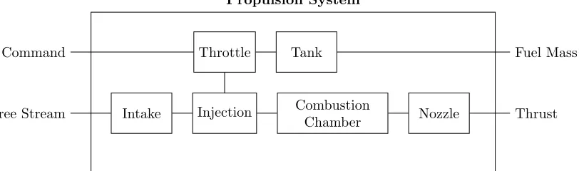
Free Stream Intake Injection Combustion

Chamber Nozzle Thrust

Throttle Tank Fuel Mass

Command

[image:10.612.107.513.510.630.2]

Propulsion System

Figure 7: Example of the modular structure of the propulsion model for a Scramjet/Ramjet.

II.E. Propulsion Model

within the MatlabR environment. This modularity brings significant flexibility to the software by allowing it to be configured to easily model many different kinds of propulsion systems. Moreover, thanks to the object oriented structure of the software, it is possible to implement every module in terms of a defined set of properties and parameters that can be changed easily during run-time. This latter feature makes the software particularly suitable for application to vehicle optimization studies.

In Fig. 7 on the previous page for instance, a schematic of the HPPMM model, structured in order to represent a scramjet/ramjet engine, is depicted. The modules can easily be changed and re-arranged to rep-resent an alternative engine configuration. Hybrid engines can be modelled by collating and interconnecting all the required modules, then switching on/off certain of the modules according to a proposed schedule of operation. Specific details of the models used to calculate the gas dynamics within each of the modules, and thus the overall engine performance, are given by Mogaveroet al.17

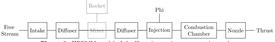
The propulsion system of the RLV that is the subject of this particular article is a Rocket Based Combined Cycle (RBCC) engine system, derived from the engine that was proposed for Hyperion, a launch vehicle conceived by the Aerospace Systems Design Laboratory at Georgia Tech.18 This engine can operate over a wide range of flight conditions by changing its configuration to allow operation in one of several different modes:

• Ejector mode

• Pure ramjet mode

• Pure rocket mode

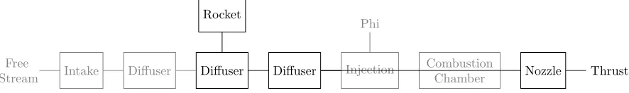
The ejector mode involves the use of an air-augmented rocket with post-combustor. The engine, when in this mode, is able to provide thrust from subsonic to low supersonic flight conditions with higher specific impulse than a conventional rocket. Once sufficient speed is attained, the rocket can be turned off in order to take advantage of the higher specific impulse of the ramjet mode. The pure rocket mode is eventually employed to provide the final boost for orbital insertion, and is adopted once the thermal limits of the ramjet are reached and the atmosphere becomes too rarefied to sustain air-breathing propulsion. A schematic of the HPPMM model for this propulsion system is depicted in Figs. 8, 9 and 10. In Table 2 the sectional areas of the engines at the conjunctions between the various modules are listed. Both the intake and the nozzle have variable geometry in order to allow the engine to adapt to its wide operational range: the table lists the maximum and minimum areas that these parts of the engine can adjust to during operation. The HPPMM propulsion module allows full control over the switching between the three propulsion modes of the engine. In the present model, the switching between modes is governed simply by the free stream conditions, in particular the Mach number and the total pressure, as delimited by the operational range for the engine in each of its modes as listed in Table 3. As can be seen, the operational ranges of the engine in its various modes overlap to some extent; the switching algorithm thus selects the appropriate mode by giving priority to the mode that is already in operation. In this way, unrealistic cycling between engine modes, particularly near the operational threshold of a particular mode, is avoided in the model.

Free

Stream Intake Diffuser Mixer Rocket

Diffuser Injection Phi

Combustion

[image:11.612.90.526.526.706.2]

Chamber Nozzle Thrust

Figure 8: HPPMM model of the Hyperion engine: ejector mode.

Free

Stream Intake Diffuser Mixer

Rocket

Diffuser Injection Phi

Combustion

Chamber Nozzle Thrust

[image:11.612.86.527.633.701.2]

Free

Stream Intake Diffuser Diffuser

Rocket

Diffuser Injection Phi

Combustion

[image:12.612.85.528.57.123.2]

Chamber Nozzle Thrust

Figure 10: HPPMM model of the Hyperion engine: pure rocket mode.

Area [m2_]

Node name Min Max

Pre-Intake 0 ∞

Intake 0 2.5084

Throat 0 0.6271

Pinch Point 0.7655 0.7655

Primary 1.0452 1.0452

Mixer End 1.0452 1.0452 Rocket Outlet 0.2796 0.2796 End Diffuser 2.0903 2.0903 Injection 2.0903 2.0903 End Chamber 2.0903 2.0903

[image:12.612.190.425.378.444.2]

Nozzle 0 8.8258

Table 2: Nodal areas within the HPPMM model of the Hyperion engine.

Mach Number p0[P a]

Mode Min Max Min Max

Ejector Mode 0 3.0 1·104 _∞

Pure Ramjet Mode 2.5 8.0 5·105 _∞

Pure Rocket Mode 0 ∞ 0 ∞

Table 3: HPPMM model of the Hyperion engine: operating ranges for each propulsion mode.

II.F. Weight Model

The weight model within HyFlow allows the mass of each individual component of the vehicle to be estimated once its flight performance, the dimensions and shape of its subsystems, and the amount of cryogenic fuel required for both the propulsion system and its ACS is known. In the present version of the module, elements of the Hypersonic Aerospace Sizing Analysis (HASA) method have been used in order to estimate the Gross Take-Off Mass (GTOM) of the vehicle. The HASA method is a statistical weight approximation technique, and, despite its lack of accuracy in the evaluation of system mass at component level, it has been shown to approximate correctly the GTOM for various types of hypersonic vehicles, including the Space Shuttle.10 The weight model within HyFlow can also compute the shift of the location of the centre of mass of the vehicle as the on-board fuel is consumed: this is an important consideration when the longitudinal stability and controllability of the vehicle is being assessed.

II.F.1. Thermal Insulation

The total mass of the TPS can be evaluated as the sum of the masses of the RSI layers applied to the vehicle’s surface together with the mass of the ACS, if employed. The mass of an RSI layer is given simply by

where δi is the thickness of the RSI material, Ai represents the surface area covered by the RSI in the

corresponding thermal zone, and ρm is the density of the insulation material. Similarly, the mass of the

ACS is approximated as the sum of the masses of its component layers of RSI, calculated using Eq. 28 on the preceding page, a basic system massm0

acs, a term proportional to the length of piping used within the

system, and the total mass of coolant,mcool, that passes through the system during the mission:

macs=

X

i=1,2

ρmAδi+m0acs+kacsLpipeNpipe+

Z tf

0

˙

mcooldt (29)

II.F.2. Propulsion System

In the present weight model, the total mass of the propulsion system is considered to be the sum of the mass of the thrust structuremthrust that supports the engines, the mass of the propulsion system itself, denoted mengines, and the mass of the fuel required by the propulsion system during the mission, denoted mf uel.

The equations for calculating these values within HyFlow are taken directly from the HASA method where

mthrustis assumed to scale with the maximum thrust that can be produced by the engines, andmengines is

based on a characteristic length of the engine, and the number of engines.

II.F.3. Packaging

The packaging module within HyFlow is responsible for the arrangement of the various system components within the internal space of the vehicle. The internal arrangement can be based on an order that is pre-defined by the user, or can be automatically set to maximize the forward location of the centre of mass of the vehicle for considerations of longitudinal stability. Additionally, the packaging module provides a means of verifying that all of the internal components, such as the tanks, subsystems and payload can be accommodated within the Inner Mould Line (IML) of the vehicle. The IML is obtained by offsetting the external mesh of the vehicle by the local TPS thickness. If the internal configuration of the vehicle does not fit within the boundaries defined by the IML, the module then automatically scales the vehicle so that it does.

III.

Baseline Trajectory

T

heselection of an appropriate set of optimisation tools for the design of vehicle trajectories is never a par-ticularly straightforward process. The convergence of conventional, simple gradient-based optimisation routines is often severely hampered by particular features that are embedded within the model for the sys-tem’s performance. Changes in behavioral mode or other discontinuities embedded within the model cause particular problems in this respect. The choice of optimisation algorithm can thus influence the outcome of the design process considerably, and it can be difficult, if not impossible, to find the true, globally-optimal design solution even if a good initial guess is available. The method used in the present work is based on a mixed approach. A population-based stochastic algorithm is used first to explore the design space and to identify a set of neighbourhoods in which candidates for the global optimum of the system might exist. A gradient-based approach is then used in each such neighbourhood to refine the solution and to ensure that the constraints on the system are accurately met.13 _{Following this, the highest ranked solution according to}

its cost function is accepted as the global optimum. To optimise the re-entry trajectory of our representa-tive RLV, a direct collocation method based on the Finite Elements in Time (FET) approach and using a spectral basis12 _{is applied: in this approach, the trajectory is discretised into a large but finite numberN}

of sub-intervals, and the design space is then the matrix product of the unit vector of dimension N and a suitable control vectorc for the vehicle along its trajectory. The resultant non-linear programming (NLP) problem14 _{is then solved using the MOPED}15 _{algorithm to search for candidate optima; these solutions are}

then refined using the gradient-based IDEA16 _{optimisation method.}

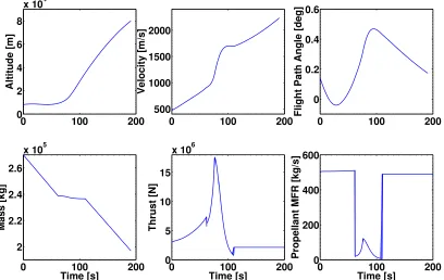
III.A. Ascent trajectory

0 100 200 0

2 4 6 8

x 104

Altitude [m]

0 100 200

500 1000 1500 2000

Velocity [m/s]

0 100 200

0 0.2 0.4 0.6

Flight Path Angle [deg]

0 100 200

2 2.2 2.4 2.6

x 105

Time [s]

Mass [kg]

0 100 200

0 5 10 15

x 106

Time [s]

Thrust [N]

0 100 200

0 200 400 600

Time [s]

[image:14.612.105.513.58.316.2]

Propellant MFR [kg/s]

Figure 11: Baseline ascent trajectory for the CFASTT-1 vehicle.

trajectory. The optimal control problem13 _{aims to maximize the payload mass on board our representative}

RLV, i.e. to find

max

c∈D mpay (30)

subject to the dynamics described in Section II.B on page 3 and initial conditions (i.e. att= 0)h0= 8.2 km,

v0 = 0.470 km/s, γ0 = 8◦,χ0 = 0◦, λ0 = 0◦, θL0 = 0◦ set to start after the transition into the supersonic

regime. The terminal conditions (i.e. at t=tf) are hf = 80 km,vf = 8.2 km/s, andγf = 0.2◦ are those

required to enter into a circular orbit at 80 km altitude. Path constraints are imposed on both the peak heat flux at the nose stagnation point, ˙qand the dynamic pressure q∞, as well as on the normal and axial

accelerations, ay and az experienced by the vehicle. The resultant baseline trajectory for the ascent into

orbit is shown in Fig. 11.

III.B. Re-entry trajectory

During the subsequent re-entry, the RLV follows an un-powered, gliding trajectory controlled by the angle of attack α and the bank angle µ. The nominal control law c(t) is then obtained as the solution of the optimisation problem which aims to minimize the integrated heat load at the nose stagnation point:11

min

c∈D

Z tf

t0

˙

qst(t)dt (31)

subject to the dynamics described in Section II.B on page 3 and initial conditions (i.e. at t = 0) set to start in the hypersonic regime: h0 = 120 km, v0 = 7.8 km/s, γ0 = −1◦, χ0 = 90◦, λ0 = 1◦, θL0 = 0◦.

The terminal conditions (i.e. at t=tf) are hf = 24 km, vf = 0.8 km/s, γf =−30◦, χf = 90◦, λf = 40◦,

andθLf = 0◦. Additional path constraints are imposed on the peak heat-flux at the nose stagnation point

˙

q < 500,000 W/m2_{, and the maximum acceleration along the normal body axis so that a}

y(t)≤ 28 m/s2.

0 200 400 600 800 20 40 60 80 100 120 Altitude [km]

0 200 400 600 800

0 2 4 6 8 Velocity [km/s]

0 200 400 600 800

0 0.1 0.2 0.3

Longitude [deg]

0 200 400 600 800

0 10 20 30 40 Latitude [deg]

0 200 400 600 800

−30 −20 −10 0

Flight Path Angle [deg]

0 200 400 600 800

90 95 100

Azimuth [deg]

0 200 400 600 800

−10 0 10 20 Accelerations [m/s 2 ] Time [s] Lateral Normal Axial

0 200 400 600 800

0 1000 2000

Aero Moments [kN.m]

Time [s] Pitch Yaw Roll

0 200 400 600 800

0 100 200 300

Max Heat−Flux [kW/m

2]

[image:15.612.79.532.52.334.2]

Time [s]

Figure 12: Baseline re-entry trajectory for the CFASTT-1 vehicle.

IV.

Design Analysis

D

ueto the strong coupling between its various subsystems (e.g. the propulsion system and the airframe structure and aerodynamics, as mentioned earlier), the task of designing an RLV is inherently multi-disciplinary: many of the design variables have a considerable mutual influence, and design objectives and constraints can be mutually conflicting to an extent which is amplified by the extremely tight tolerances on vehicle performance that need to be achieved. It becomes essential thus to be able to quantify, as early on in the design process as is possible, the effects of uncertainty in some of the key design variables in order to provide reliable estimates of the margins on the likely performance of the vehicle. The advantage of the use of a low-order but comprehensive parametric model for preliminary design, such as the HyFlow system that was introduced in section II on page 2, is of course the ease with which parametric variations in the properties of the vehicle system can be explored.

Two fundamentally different types of uncertainty are inherent to the system. The first type is the stochas-tic uncertainty (also called random uncertainty) that is associated with inherent variations in the physical system or its environment. An example would be the natural variability in the properties of the material used to construct the layers of TPS on the vehicle, or the natural fluctuations in atmospheric temperature at a particular altitude because of turbulence and winds. A second, perhaps even more important type of uncertainty in the context of design is however the epistemic uncertainty that results from the use of inadequate, incomplete or even erroneous physical models to encapsulate the behaviour of the system.

IV.A. Material Properties

Variability in the thermal properties of the materials used to construct the TPS of the vehicle can have a significant impact on the temperature that its surface attains during operation.1 _{The combined influence of}

uncertainties in the TPS surface emissivity tps (i.e. on the amount of radiative cooling that takes place),

specific heat ctps, and conductivity ktps on the thermal response predicted by our TPS model has been

investigated using a Monte-Carlo analysis with 1000 optimization runs set up to design a passive thermal insulator for the leading edge of the wings of our representative RLV. The TPS was assumed to be composed from a layer of Reinforced Carbon-Carbon (RCC) insulation material in order to retain the temperature of the underlying structure below 500 K for the duration of the re-entry. A uniform distribution of material properties with a ±20% deviation around their nominal values was adopted in order to characterise the inherent variability in the fabrication of the TPS together with the possibility of thermal degradation and mechanical damage during the previous flight history of the craft. The results of this Monte-Carlo analysis, presented in Fig. 13, shows that this assumption results in a distribution of predicted TPS optimal thicknesses about a nominal value of 96.8 mm (see Fig. 15 on the next page). Statistical analysis (see Fig. 14 on the following page) then suggests that if the assumed variability in material properties is accurate, then designing the system to the predicted nominal TPS thickness would result in higher than nominal heating of the structure of the vehicle on 45% of missions, but that, if a design margin of, say, 110% of nominal was adopted, then the likelihood of the system not meeting its specified performance would be very small indeed. The great advantage of the statistical process is that it allows the safety margins and required design tolerances on the system to be revealed in this way, allowing adequate margins to be incorporated into the design or, alternatively, focusing attention on those elements of the system that need to be better quantified before the design can proceed to fruition.

0.088 0.09 0.092 0.094 0.096 0.098 0.1 0.102 0.104

0 0.005 0.01 0.015 0.02 0.025 0.03 0.035

PDF

Thickness [m] Discrete

[image:16.612.77.530.350.601.2]

Nominal

Figure 13: Results of a 1000-sample Monte-Carlo simulation of the performance of the leading edge TPS

along the nominal trajectory. The TPS material is assumed to be Reinforced Carbon-Carbon (RCC) with stochastic emissivity = 0.79±20%, specific heat cm = 0.770 kJ/(kg.K)±20%, and conductivity km =

0.0860 0.088 0.09 0.092 0.094 0.096 0.098 0.1 0.102 0.104 0.1

0.2 0.3 0.4 0.5 0.6 0.7 0.8 0.9 1

Optimal Thickness [m]

Probability

CDF

[image:17.612.123.486.68.300.2]

Nominal

Figure 14: CDF curve for the optimal TPS thickness.

0 100 200 300 400 500 600 700 800

300 400 500 600 700 800 900 1000 1100 1200

Time [s]

Temperature [K]

TPS − node 1 TPS − node 2 TPS − node 3 TPS − node 4 TPS − node 5 TPS − node 6 Structure Node Max Temperature Empty Pipe Node

Figure 15: Thermal performance of a passive TPS with a nominal optimal thickness of about 10 cm.

IV.B. Active Cooling System

[image:17.612.118.477.357.564.2]

been modelled, allowing the ACS to be switched on or off when the temperature of the underlying structural skin of the vehicle attains a prescribed threshold value. In the results presented here, the skin was assumed to consist of 2 mm thick titanium, and the threshold was set to include a 10% margin below the material’s critical temperature (here assumed to be 500 K) to account for thermal inertia within the structure. The mass flow rate of coolant ˙mcoolwas held constant at 5 kg/s when the ACS system was switched on, and the

hydraulic diameter of the ACS feeder pipes was set to 5 cm.

A more comprehensive analysis than that presented here would be required in order to evaluate the optimal combination of design parameters that result in the most efficient and lightweight thermal protection system for the vehicle. Similarly, a more sophisticated control system for the flow rate through the system could be adopted in order to reduce the cyclic thermal loads that the present control strategy induces in the structure throughout the duration of the re-entry trajectory. These extensions to the models described here, in particular the use of a more sophisticated control model for the coolant flow rate, would be relatively straightforward to implement, and the results presented here serve thus simply to demonstrate the capabilities of the TPS module within HyFlow.

In designing a simple ACS for the leading edges of the wings which allows straightforward comparison with the performance of an equivalent passive TPS, the example of the previous section was modified by reducing the overall thickness of the RCC layer from its nominal optimal thickness of 96.8 mm to a value of 60 mm, creating two layers of 3 cm-thick RCC, denoted TPS1 and TPS2, one on either side of the ACS feeder lines (see Fig. 3 on page 6: in the present example, node 1 is at the surface of the vehicle, node 2 is within TPS1, node 3 and node 4 are in contact with the coolant pipe lines, node 5 is within TPS2, and node 6 is at the interface between TPS2 and the vehicle structure). As a point of comparison, the performance of the system with the ACS switched off entirely during the descent is depicted in Fig. 16. As can be seen in the figure, the temperature within the structure rises to about 800 K by the end of the descent, and thus the thermal management system, at least when operated in this passive mode, clearly does not meet the design requirement that the temperature of the structure be maintained below 500Kfor the duration of the mission.

0 100 200 300 400 500 600 700 800

200 300 400 500 600 700 800 900 1000 1100 1200

Time [s]

Temperature [K]

[image:18.612.100.506.386.621.2]

TPS1 − node 1 TPS1 − node 2 TPS1 − node 3 − ACS TPS2 − node 4 − ACS TPS2 − node 5 TPS2 − node 6 Structure node Max Temperature ACS on/off Temperature

Figure 16: Thermal performance of a passive TPS with a reduced thickness of about 6 cm.

its critical temperature until a point at aboutt= 650 s into the descent where, due to boil-off, all the cryogen within the tank has been consumed. Thereafter, the TPS continues to act as a passive thermal shield for the remainder of the trajectory. This cooling strategy results in the structural temperature reaching 580 K by the end of the re-entry path. Despite a significant reduction in the temperature of the structure as compared to a fully passive TPS of the same thickness, this system also does not meet the design requirements.

0 100 200 300 400 500 600 700 800

300 400 500 600 700 800 900 1000 1100 1200

Temperature [K]

0 100 200 300 400 500 600 700 800

20 22 24 26

Temperature [K]

0 100 200 300 400 500 600 700 800

0 20 40 60

Time [s]

Volume [m

3]

TPS1 − node 1 TPS1 − node 2 TPS1 − node 3 − ACS TPS2 − node 4 − ACS TPS2 − node 5 TPS2 − node 6 Structure Node Max Temperature ACS on/off Temperature

Tank Node

[image:19.612.82.500.136.394.2]

Coolant

Figure 17: Thermal performance of an Active Cooling System with a coolant reserve of 50m3_.

Figure 18 on the next page shows the behaviour of the same system as before, but when instead 80 m3 of cryogen is made available to the ACS. In this case, the ACS manages to keep the temperature of the structural skin within the desired limits throughout the duration of the re-entry, even though all the cryogen is still consumed shortly before the end-point of the descent is reached. Despite the simplicity of the thermal management system modelled here, these results illustrate the ability of the TPS module within HyFlow to enable the type of parametric studies and trade-offs between options that would be necessary for the effective and robust multi-disciplinary design optimisation of any future Reusable Launch Vehicle.

IV.C. Ground-hold Analysis

As discussed in Section II.D on page 9, the TPS of the vehicle must be designed not only to protect the vehicle from the thermal loads experienced in flight, but also during those times when the vehicle is being held on the ground prior to a mission and its tanks are full of cryogenic fuel. The danger is that cooling of the structure might result in the build-up of a layer of ice on the outer surface of the vehicle. To model this phenomenon using the thermal module within HyFlow, a 20 metre-long integral tank, containing a volume of 420 m3 _{of fuel and located within the forward fuselage of the CFASTT-1 vehicle, was assumed to be}

0 100 200 300 400 500 600 700 800 200

300 400 500 600 700 800 900 1000 1100 1200

Temperature [K]

0 100 200 300 400 500 600 700 800

20 22 24 26

Temperature [K]

0 100 200 300 400 500 600 700 800

0 50 100

Time [s]

Volume [m

3]

TPS1 − node 1 TPS1 − node 2 TPS1 − node 3 −ACS TPS2 − node 4 − ACS TPS2 − node 5 TPS2 − node 6 Structure Node Max Temperature ACS on/off Temperature

Tank Node

[image:20.612.77.535.57.318.2]

Coolant

Figure 18: Thermal performance of an Active Cooling System with a coolant reserve of 80m3_.

0 1000 2000 3000 4000 5000 6000 7000

0 50 100 150 200 250 300

Time [s]

Temperature [K]

TPS1 Node

TPS2 Node

Structure Node

Insulation Node

Tank Node

Figure 19: Evolution of the nodal temperatures during ground-hold operations.

[image:20.612.118.479.370.611.2]

0 1000 2000 3000 4000 5000 6000 7000 0

1 2 3 4 5 6

Time [s]

Thickness [mm]

[image:21.612.117.498.66.318.2]

ice layer thickness

Figure 20: Growth of the ice layer during ground-hold operations.

approximately 55 kg per square metre of surface area covered (this amount of ice could potentially increase the GTOM of the CFASTT-1 vehicle by about 414 kg even if only the forward-fuselage strakes were to be coated). If, instead, the passive TPS considered in section IV.A on page 16 were to cover the vehicle (in other words a system consisting of a 10 cm thick layer of RCC instead of a 6 cm layer) then, as shown in Figs. 21 on the next page and 22 on the following page the ice first begins to appear about 50 minutes after the ground-hold phase has started, and the layer reaches a thickness of only 3 cm (i.e. about 225 kg added to the GTOM of the CFASTT-1 vehicle) after two hours. This comparison reveals a rather interesting mechanism whereby a lightweight, advanced cooling system, designed for maximum in-flight performance, may in fact become somewhat of a liability when the formation of ice during the ground-hold element of the mission is considered. The resolution this conundrum is not entirely apparent as yet - certainly the obvious route of increasing the thickness of the insulating layer between the tank and the structural skin would appear to be at least partially self-defeating.

IV.D. Atmospheric Model

The natural variation of the thermodynamic properties of the atmosphere about their nominal values is a major source of uncertainty in the prediction of the performance of any trans-atmospheric vehicle. This uncertainty is represented in HyFlow by treating the atmospheric temperature profile, T∞(h), where h

denotes altitude above sea level, as a random variable. More specifically, if the nominal temperature profile within the atmosphere is denoted asTnom

∞ (h), then a representation of the temperature profile in the presence

of uncertainty is constructed as

T∞(h) =T∞nom(h) +ε(h)S(h) (32)

In this expression,εis an error bound function which captures the statistical variance of the temperature with altitude. This function can, at least in principle, be determined from measurement. For present purposes, and in the absence of better information,εis modelled very simply by linear interpolation between assumed bounds εL andεU on the uncertainty at the lower (h= 0) and upper (h =hU) edges of the atmosphere,

respectively, so that

0 1000 2000 3000 4000 5000 6000 7000 0

50 100 150 200 250 300

Time [s]

Temperature [K]

TPS 1 node

TPS 2 node

Structure Node

Insulation Node

[image:22.612.107.480.61.303.2]

Tank Node

Figure 21: Evolution of the nodal temperatures during ground-hold operations for the nominal optimal

TPS thickness.

0 1000 2000 3000 4000 5000 6000 7000

0.5 1 1.5 2 2.5 3 3.5

Time [s]

Thickness [mm]

ice layer thickness

Figure 22: Growth of the ice layer during ground-hold operations for the nominal optimal TPS thickness.

[image:22.612.114.499.365.617.2]

a direct simulation of its likely performance. Finally, the variability that is introduced into the free-stream temperature using this approach are propagated into the remainder of the atmospheric model by imposing the ideal gas law and barostatic equilibrium. A typical variation of the atmospheric properties with altitude generated using this approach is shown in Fig. 23.

0 20 40 60 80 100 120

0 50 100 150 200

Pressure [kPa]

Altitude [km]

0 200 400 600 800 1000 1200 1400 0

50 100 150 200

Temperature [K]

Altitude [km]

−0.20 0 0.2 0.4 0.6 0.8 1 1.2 50

100 150 200

Density [kg/m3]

Altitude [km]

9.2 9.3 9.4 9.5 9.6 9.7 9.8 9.9 0

50 100 150 200

Gravity [m/s2]

Altitude [km]

2600 280 300 320 340 360 50

100 150 200

Speed of Sound [m/s]

Altitude [km]

0 2 4 6 8 10

0 50 100 150 200

Knudsen Number [−]

[image:23.612.91.527.120.388.2]

Altitude [km]

Figure 23: 1976 US Standard Atmosphere subject to uncertainty in the temperature variation with altitude

(nominal atmospheric conditions in red). The uncertainty in the atmospheric temperature is taken to vary from 10% of the nominal value (at sea level) to 30% at 200 km altitude.

20 21 22 23 24 25 26 27 0 0.1 0.2 0.3 0.4 0.5 0.6 0.7 0.8 0.9

Final Altitude [km]

PDF discrete Parzen Gaussian Nominal Mean Final Altitude

0.75 0.8 0.85 0.9 0.95 0 5 10 15 20 25 30

Final Velocity [km/s]

[image:24.612.84.544.56.208.2]

discrete Parzen Gaussian Nominal Mean Final Velocity

Figure 24: PDF of the final states when the nominal schedules of bank angleµand angle of attackαare

integrated using a perturbed atmospheric model.

0 5 10 15 20

x 10−3 0 50 100 150 200 250 300

Final longitude [deg]

PDF discrete Parzen Gaussian Nominal Mean Final Longitude

39.2 39.4 39.6 39.8 40 40.2 40.4 40.6 0 0.5 1 1.5 2 2.5 3 3.5 4 4.5

Final Latitude [deg]

[image:24.612.77.543.264.415.2]

discrete Parzen Gaussian Nominal Mean Final Latitude

Figure 25: PDF of the final states when the nominal schedules of bank angleµand angle of attackαare

integrated using a perturbed atmospheric model.

−36 −34 −32 −30 −28 −26 0 0.1 0.2 0.3 0.4 0.5 0.6 0.7

Final Flight Path Angle [deg]

PDF discrete Parzen Gaussian Nominal Mean

Final Flight Path Angle

96 96.5 97 97.5 98 98.5 99 99.5 100 0 0.2 0.4 0.6 0.8 1 1.2 1.4 1.6

Final Heading Angle [deg]

discrete Parzen Gaussian Nominal Mean

Final Heading Angle

Figure 26: PDF of the final states when the nominal schedules of bank angleµand angle of attackαare

integrated using a perturbed atmospheric model.

IV.E. Engine Parameters

[image:24.612.79.548.467.621.2]

feasibility of the nominal ascent trajectory, presented in section III on page 13, of varying the mixer efficiency of the engine when in ejector mode, the Mach number at which the system switches from Ejector to Ramjet mode, and the relative size of the rocket and ramjet components of the propulsion system of the vehicle, are presented below.

Figure 27 illustrates the sensitivity of the ascent trajectory to the relative size of the rocket and ramjet components of the propulsion system. The aim of the analysis is to assess the performance of the system under the tradeoff where the propulsion system, at the extremes of the analysis, is either predominantly air-breathing or predominantly rocket-like in its behaviour. The overall size of the engine was thus increased (or decreased) by 30% while the rocket size, and consequently the mass flow rate of its propellant, was correspondingly decreased (or increased) by the same percentage. As can be seen, the adoption of an over-sized ramjet results in a slight gain in final payload mass over the nominal case, but at the expense of extremely poor performance early on in the vehicle’s trajectory. In the opposing situation where the rocket is enlarged, the time taken to ascend to orbit is significantly extended, and, as a result of the low effective specific impulse of the propulsion system in this configuration, there is a significant loss in payload performance. Put simply, the undersized ramjet is close to being just a simple rocket, and allows very little advantage to be gained at all from the combined-cycle configuration of the powerplant. In comparison, the over-sized design might, at least at first glance, seem very attractive even in comparison to the baseline configuration. The effect of increasing the size of the engine on the remainder of the vehicle design needs to be borne in mind very clearly, however, particularly given the multi-disciplinary focus of the present study.

0 100 200 300 0

2 4 6 8

x 104

Altitude

0 100 200 300 0

1000 2000 3000 4000 5000 6000

Velocity

0 100 200 300 −0.2

0 0.2 0.4 0.6

Flight Path Angle

0 100 200 300 0.5

1 1.5 2 2.5

3x 10 5

Time [s]

Mass

0 100 200 300 0

1 2 3 4x 10

7

Time [s]

Thrust

0 100 200 300 0

100 200 300 400 500 600 700

Time [s]

Propellant MFR

Nominal

[image:25.612.84.533.294.599.2]

Ramjet +30% Rocket −30% Ramjet −30% Rocket +30%

Figure 27: Sensitivity of the ascent trajectory to the relative size of the rocket and ramjet components of

the propulsion system.

number at which the system switches from ejector to ramjet mode earlier in its ascent. It is also clear however that, with the engine in ejector mode, the vehicle climbs faster the higher its mixer efficiency, with the interesting consequence that the engine when in its subsequent ramjet phase produces a lower thrust, resulting overall in a reduction in the performance of the vehicle. Indeed, a vehicle with too high a mixer efficiency appears to be unable to reach its target altitude; in comparison, the vehicle with mixer efficiency just 15% greater than nominal reaches its 80 km with a small time delay and with a lower final mass than the nominal case. It should be borne in mind however when assessing these results that the calculations presented here were all performed using the same control laws, i.e. those that were established for the nominal trajectory of the vehicle, and that re-optimisation of these laws for the vehicle with its off-nominal propulsion system would most likely allow it to better balance the improved ejector performance with the exploitation of the various operational modes of the engine. It is indeed interesting to note the large reduction in fuel consumption during the ejector phase that results from an improvement in the powerplant’s mixer efficiency. It is possible to speculate that this reduction in fuel consumption could be translated into a large gain in payload mass fraction at the end of the ascent simply by employing a set of control laws that are better suited to the engine’s operational characteristics. By comparison, the inferences from the data when the mixer efficiency is lower than nominal are much more straightforward: it is clear that the ejector performance in this case is so poor that the transition to Ramjet mode is delayed too late into the ascent for this part of the propulsion system to be effective in accelerating the vehicle up to its orbital speed and altitude.

0 50 100 150 200

0 2 4 6 8

x 104

Altitude [m]

0 50 100 150 200

0 500 1000 1500 2000 2500

Velocity [m/s]

0 50 100 150 200

−0.2 −0.1 0 0.1 0.2 0.3 0.4 0.5

Flight Path Angle [deg]

0 50 100 150 200

1.8 2 2.2 2.4 2.6

x 105

Time [s]

Mass [kg]

0 50 100 150 200

0 5 10 15

x 106

Time [s]

Thrust [N]

0 50 100 150 200

0 100 200 300 400 500 600

Time [s]

Propellant MFR [kg/s]

[image:26.612.87.531.281.586.2]

Nominal MixEff +30% MixEff +15% MixEff −15%

Figure 28: Sensitivity of the ascent trajectory to the mixer efficiency of the engine when in ejector mode.

vehicle’s trajectory: the performance of the propulsion system is better matched at the transition between Ejector and Ramjet modes, as can be inferred from the associated reduction in the size of the discontinuity in the thrust produced by the system at the mode-switch, and the vehicle is able to reach its final target altitude earlier with a slight gain in terms of overall mass to orbit. Although these observations and potentialities all need to be seen in the light of more general considerations of the vehicle’s performance and operability, the results presented here again show clearly the benefits of reduced-order modelling in being able to trade and compare various aspects of the performance of the vehicle, and indeed thus to be able to inform early design decisions regarding the key parameters that will govern its eventual configuration.

0 50 100 150 200

0 2 4 6 8

x 104

Altitude [m]

0 50 100 150 200

500 1000 1500 2000

Velocity [m/s]

0 50 100 150 200

−0.1 0 0.1 0.2 0.3 0.4 0.5 0.6

Flight Path Angle [deg]

0 50 100 150 200

1.9 2 2.1 2.2 2.3 2.4 2.5 2.6 2.7x 10

5

Time [s]

Mass [kg]

0 50 100 150 200

0 0.5 1 1.5

2x 10 7

Time [s]

Thrust [N]

0 50 100 150 200

0 100 200 300 400 500 600

Time [s]

Propellant MFR [kg/s]

[image:27.612.88.528.166.462.2]

Nominal M=3 Switch M=3.5 Switch M=2.5

Figure 29: Sensitivity of the ascent trajectory to the Mach number at which the system switches from

Ejector to Ramjet mode.

V.

Conclusion