Molecular dynamics in arbitrary geometries : parallel evaluation of pair forces

Department of Mechanical Engineering, University of Strathclyde, Glasgow G1 1XJ, UK

(draft August 14, 2007)

A new algorithm for calculating intermolecular pair forces in Molecular Dynamics (MD) simulations on a distributed parallel computer is presented. The Arbitrary Interacting Cells Algorithm (AICA) is designed to operate on geometrical domains defined by an unstructured, arbitrary polyhedral mesh that has been spatially decomposed into irregular portions for parallelisation. It is intended for nano scale fluid mechanics simulation by MD in complex geometries, and to provide the MD component of a hybrid MD/continuum simulation. The spatial relationship of the cells of the mesh is calculated at the start of the simulation and only the molecules contained in cells that have part of their surface closer than the cut-off radius of the intermolecular pair potential are required to interact. AICA has been implemented in the open source C++ code OpenFOAM, and its accuracy has been indirectly verified against a published MD code. The same system simulated in serial and in parallel on 12 and 32 processors gives the same results. Performance tests show that there is an optimal number of cells in a mesh for maximum speed of calculating intermolecular forces, and that having a large number of empty cells in the mesh does not add a significant computational overhead.

Keywords:molecular dynamics, nano fluidics, hybrid simulation, intermolecular force calculation, parallel computing PACS: 31.15.Qg, 47.11.Mn

1 Introduction and Motivation

1.1 MD Simulation in Arbitrary Geometries

Simulations of nano scale liquid systems can provide insight into many naturally-occurring phenomena, such as the action of proteins that mediate water transport across biological cell membranes [1]. They may also facilitate the design of future nano devices and materials (e.g. high-throughput, highly selective filters or lab-on-a-chip components). The dynamics of these very small systems are dominated by surface interactions, due to their large surface area to volume ratios. However, these surface effects are often too complex and material-dependent to be treated by simple phenomenological parameters [2] or by adding ‘equivalent’ fluxes at the boundary [3]. Direct simulation of the fluid using molecular dynamics (MD) presents an opportunity to model these phenomena with minimal simplifying assumptions.

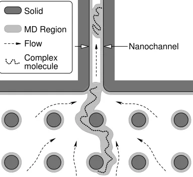
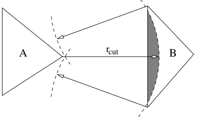
Some MD fluid dynamics simulations have been reported [4, 5, 6, 7, 8], but MD is prohibitively com-putationally costly for simulations of systems beyond a few tens of nanometers in size. Fortunately, the molecular detail of the full flow-field that MD simulations provide is often unnecessary; in liquids, beyond 5–10 molecular diameters (. 3nm for water) from a solid surface the continuum-fluid approximation is valid and the Navier-Stokes equations with bulk fluid properties may be used [2, 9, 10]. Hybrid simulations have been proposed [11, 12, 13, 14] to simultaneously take advantage of the accuracy and detail provided by MD in the regions that require it, and the computational speed of continuum mechanics in the regions where it is applicable. An example application of this technique is shown schematically in figure 1, where a complex molecule is being electrokinetically transported into a nanochannel for separation and iden-tification [15]. Only the complex molecule, its immediately surrounding solvent molecules, and selected near-wall regions require an MD treatment; the remainder of the fluid (comprising the vast majority of the volume) may be simulated by continuum mechanics. A hybrid simulation would allow the effect of different complex molecules, solvent electrolyte composition, channel geometry, surface coatings and electric field strengths to be analysed at a realistic computational cost.

Solid

molecule Complex Flow MD Region

Nanochannel

Figure 1. Schematic of an application of a hybrid MD/continuum simulation: complex molecules being transported into a nano channel. Only the complex molecules, regions near them and regions near solid surfaces need an MD treatment; the remaining volume

can be simulated with continuum mechanics.

Figure 2. Left:A complex geometry test case. A three-inlet fluid mixing channel with a wall volume for explicit crystalline molecular walls. The overall height is 82nm. The geometry was generated using Pro/ENGINEERR_{CAD software, exported to and meshed using}

GAMBITR, then imported into OpenFOAM, filled with 2167110 molecules and the MD simulation run using_gnemdFOAM(see

section 3).Right:The mesh has been decomposed into 52 portions for parallel processing. The 48148 molecules contained in one portion are shown. Two different types of molecule are used: wall molecules (light) are tethered in an FCC crystal and liquid molecules

(dark) which are free to move.

1.2 Neighbour List Limitations

The conventional method of MD force evaluation in distributed parallel computation is to use the cells algorithm to build neighbour lists for interacting pairs [18, 19]. Thereplicated molecule method provides interactions across periodic boundaries and interprocessor boundaries, where the system has been spatially partitioned [20, 21].

The spatial location of molecules in MD is dynamic, and hence not deducible from the data structure that contains them. A neighbour list defines which pairs of molecules are within a certain distance of each other and so need to interact via intermolecular forces. When considering systems where the geometry is defined by a mesh of unstructured, arbitrary polyhedral cells, that may have been divided into irregular and complex mesh segments for parallelisation, neighbour lists have two limitations:

(i) Interprocessor molecule transfers:A molecule may cross an interprocessor boundary at any point

in time (even part of the way through a timestep), at which point it should be deleted from the processor it was on and an equivalent molecule created on the processor on the other side of the boundary. Given that neighbour lists are constructed as lists of array indices, references or pointers to the molecule’s location in a data structure, deleting a molecule would invalidate this location and require searching to remove all mentions of it. Likewise, creating a molecule would require the appropriate new pair interactions to be identified. Neither is practical due to the computational cost involved. It is conventional to allow molecules to stray outside of the domain controlled by a processor and carry out interprocessor transfers (deletions and creations) during the next neighbour list rebuild. This is straightforward when the spatial region associated with a processor can be simply defined by a function relating a position in space to a particular cell on a particular processor (i.e. a uniform, structured mesh, representing a simple domain). In a geometry where the space in question is defined by a collection of individual cells of arbitrary shape, this is more difficult. For example, the location the molecule has strayed to may be on the other side of a solid wall on the neighbour processor, or across another interprocessor boundary.

(ii) Spatially resolved flow properties: MD simulations used for flow studies must be able to spatially

resolve fluid mechanical and thermodynamical fields. This is achieved by accumulating and averaging measurements of the properties of molecules in individual cells of the same mesh that defines the geometry. If a molecule is allowed to stray outside of the domain controlled by a processor, as above, then it would not be unambiguous and automatic which cell’s measurement the molecule should contribute to.

Both of these problems could be mitigated by communicating with the neighbouring processor to deter-mine which cell a molecule outside the domain should be in and sending its information, or alternatively maintaining a local copy of the appropriate thickness layer of geometry of the neighbouring processors. In this work, however, it has been deemed that either of these options would result in an inflexible arrange-ment, with each additional simulation feature requiring special treatment; so neighbour lists have not been used.

Neighbour lists have some unfavourable features that limit their computational speed in large and non-equilibrium simulations. If one region of the fluid has a high temperature or high velocity, then the high molecular velocities will cause the neighbour list to be invalidated and rebuilt often, limiting the calculation speed in the whole domain. Increasing the size and temperature of a system will also reduce the number of timesteps a neighbour list is valid for, thereby increasing the computational cost. This relationship can be predicted, see appendix A.

00000000 00000000 00000000 00000000 00000000 00000000

11111111 11111111 11111111 11111111 11111111 11111111

0000 0000 0000 0000 0000 0000 0000 0000 0000 0000 0000 0000 0000 0000 0000 0000

1111 1111 1111 1111 1111 1111 1111 1111 1111 1111 1111 1111 1111 1111 1111 1111

0000 0000 0000 0000 0000 0000 0000 0000 0000 0000 0000 0000 0000 0000 0000 0000

1111 1111 1111 1111 1111 1111 1111 1111 1111 1111 1111 1111 1111 1111 1111 1111 00000000

00000000 00000000 00000000 00000000 00000000

11111111 11111111 11111111 11111111 11111111 11111111

00 00 00 00

11 11 11 11

cut

r

Figure 3. Interacting cell identification example using 2D unstructured triangular cells. The spatial domain (main square section comprising the real cells) is periodic top-bottom and left-right. Real cells withinrcutthat interact with the CIQ (dark) are shaded in

grey. The required referred cells are hatched in alternate directions according to which boundary they have been referred across. Realistic systems would be significantly larger compared torcutthan shown here.

2 Arbitrary Interacting Cells Algorithm (AICA)

2.1 Interacting Cell Identification

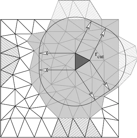
The new Arbitrary Interacting Cells Algorithm (AICA) we propose here is a generalisation of the Con-ventional Cells Algorithm (CCA) [18, 19]. In the CCA, a simple (usually cuboid) simulation domain is subdivided into equally sized cells. The minimum dimension of the CCA cells must be greater than rcut, the cut-off radius of the intermolecular pair potential, so that all molecules in a particular cell interact with all other molecules in their own cell and with those in their nearest neighbour cells (i.e. those they share a face, edge or vertex with — 26 in 3D). Extensions to this that permit the use of smaller cells [22, 23, 24] have been proposed, but they still require the domain to comprise a structured mesh of uniform cubes or cuboids. The objective of any cell algorithm is to evaluate interactions between as few molecules as possible that are further apart thanrcut to maximise computational speed.

AICA uses a 3D mesh of unstructured polyhedra, as would be used in CFD to define the geometry of a region. There are no restrictions on cell size, shape or connectivity. A cell’s position in the mesh structure does not imply anything about its physical location or connectivity. Therefore, the ability to handle arbitrary geometries comes from deducing locally which cells are in the interaction range. Each cell has a unique list of other cells that it is to interact with, this list is known as the Direct Interaction List (DIL) for the Cell In Question (CIQ). It is constructed by searching the mesh to create a set of cells that have at least one part of their surface within a distance of rcut from the surface of the CIQ, see figure 3.

Where there are multiple molecular species present with different values ofrcut, the maximum value is used to determine cell interactions. Where substantially different cut-off radii are present, it would be possible to have separate DILs for different range interactions, all of which could be constructed simultaneously using a single evaluation of the mesh.

This work has been carried out on the basis that the mesh is static. It is possible to use the same methods for a system with a dynamic mesh, providing that the information about which cells interact can be efficiently and reliably kept up-to-date, or rebuilt without incurring an unreasonable computational cost.

rcut A

Replicated molecules

Processor 2 Processor 1

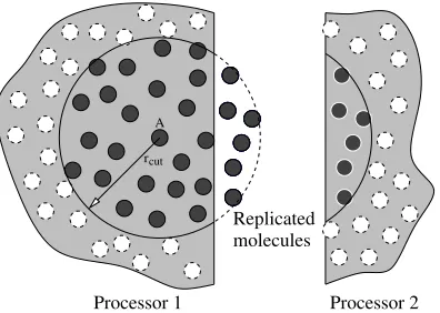
Figure 4. Spatial decomposition for parallel processing. Molecule A must calculate intermolecular forces with all other molecules within its cut-off radius,rcut. When the domain has been decomposed, some of these molecules may lie on a different processor. In this

case, copies of the appropriate molecules from processor 2 are made on processor 1.

Replicated molecules rcut

B

Figure 5. Periodic boundaries. Molecule B must calculate intermolecular forces with all other molecules withinrcut. Some of those

molecules may be on a periodic image of the system, which, in computational terms, will reside on the other side of the domain. Serial calculations in simple geometries typically use the minimum image convention [18, 19], but this is not suitable for parallelisation.

molecules in that cell and consults the cell’s DIL to find which other cells contain molecules it should interact with. Information is required to be maintained at all times stating which cell a molecule is in — this has been implemented in a robust and efficient manner in OpenFOAM as part of the methods for tracking particle motion [17].

2.2 Replicated Molecule Periodicity and Parallelisation

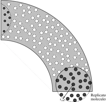
When parallelising an MD simulation, the spatial domain is decomposed and each processor is given responsibility for a single region [18]. Molecules that cross the boundaries between these regions need to be communicated from one processor to the next. Processors also communicate when carrying out intermolecular force calculations, in which molecules close to processor boundaries need to be replicated on their neighbours to provide interactions. This process is illustrated in figure 4. Periodic boundaries also require information about molecules that are not physically adjacent in the domain (see figure 5); these required interactions can also be constructed by creating copies of molecules outside the boundary.

It is possible to handle processor and periodic boundaries in exactly the same way, because they have the same underlying objective: molecules near to the edge of a region need to be copied either between processors or to other locations on the same processor at every timestep to provide interactions. This is a useful feature because decomposing a mesh for parallelisation will often turn a periodic boundary into a processor boundary. The issue is: how to efficiently identify which molecules need to be copied, and to which location, because this set continually changes as the molecules move.

rcut molecules

Replicated

Figure 6. An example of a non-parallel, separated boundary. This could represent either a 90◦_{bend in a channel where molecules are}

‘recycled’ from inlet to outlet. It could also represent a cross section through a hybrid simulation of flow in a pipe where the MD section is an outer annulus and rotational symmetry has been exploited to simulate only a quarter of the pipe — a typical CFD

technique. In both cases, molecules near the separated boundaries must correctly exchange intermolecular forces.

2.2.1 Referred Molecules and Cells. Replicated molecule parallelisation and periodic boundaries are handled in the same way usingreferred cells (see figure 3) andreferred molecules.

Referred molecule. A copy of a real molecule that has been placed in a region outside a periodic or processor boundary in order to provide the correct intermolecular interaction with molecules inside the domain. A referred molecule holds only its own position and id (i.e. identification of which type of molecule it is for multi-species simulations). Referred molecules are created and discarded at each timestep, and do not report any information back to their source molecules. Therefore if moleculej on processor 1 needs to interact with molecule k on processor 2, a separate referred molecule will be created on each processor.

Referred cell. Referred cells define a region of space and hold a collection of referred molecules. Each referred cell knows

• which real cell in the mesh (on which processor) is its source;

• the required transformation to refer the positions and orientations of the real molecules in the source cell to the referred location. A general transformation of position and orientation is required for the cases mentioned in section 2.2 and figure 6 which require the replicated cells to have a different orientation to their source cell;

• the positions of all of its own vertices. These are the positions of the vertices of the source cell which have been transformed by the same referring transform as the referred molecules it contains;

• the structure of all of the cell edges. Each edge is defined by a pair of indices in the referred vertex positions list indicating the vertices that comprise it;

• the structure of all of the cell faces. Each face is defined by a list of indices in the referred vertex positions list indicating the vertices that comprise it;

• which real cells are in range of this particular referred cell and hence require intermolecular interactions to be calculated. This is constructed once at the start of the simulation in the same way as the DIL for real-real cell interactions.

2.3 Interacting Cell Identification Methods

B

A rcut

Figure 7. Errors caused by cut-off radius searching from vertices only. A sphere of radiusrcutdrawn from the indicated vertex on cell

A intersects a face of cell B, therefore, molecules near this vertex should interact with molecules in the shaded region. A sphere of radiusrcutdrawn from either of the indicated vertices on cell B will not intersect any point of the surface of cell A, therefore,

point-face searches are not reciprocal.

2.3.1 Point-Point (PP). The fastest and most straightforward method of determining whether cells are withinrcutis to use Point-Point (PP) searching. All of theNp points in the mesh are compared to each

other using a non-double-counting loop, and if any pair of points are withinrcut of each other, then all of

the cells that these points form part of1 _{must all be in range of each other, see algorithm 1. Note that a}

point is compared to itself (pj =pi is used for the inner loop rather than pj =pi+ 1) — this guarantees

that neighbouring cells are identified for interaction if none of their non-shared vertices are within range of each other.

Algorithm 1Point-Point cell searching

forpi= 0; pi < Np;pi+ 1do

for pj =pi;pj < Np;pj+ 1 do

if the magnitude of the separation of the points referenced by pi and pj ≤rcut then

all cells whichpj andpi form part of must interact.

end if end for end for

It is possible for PP to introduce errors, where molecules that should interact do not because their containing cells are not identified as being in range. Slices of cells may not be identified for interaction because

• a vertex may be within rcut of a face of another cell, but not of any vertex. See figure 7;

• the edges of two cells may be withinrcut of each other, but none of the vertices of either cell are within

rcutof a vertex, edge or face of the other. See figure 8, this problem is only possible in 3D.

Both of these problems are most prevalent in meshes of tetrahedral cells, and cannot occur in regular meshes with perfectly, or nearly-perfectly cuboid cells.

2.3.2 Point-Point with Guard Radius (PPGR). The errors identified with the PP method can be reduced by adding a guard radius, rG to rcut. PPGR works exactly as PP, except cells with vertices separated by≤rG+rcutnow also interact. The guard radius will mean that many cells will have DILs that

are larger than necessary, which will slow down the running of the simulation because more unnecessary molecule pairs will be evaluated at each time step. It is possible to remove all errors from PP by adding a large enough guard radius, but this value is difficult to determine in advance, and in practice is relatively large, introducing a significant running performance penalty.

1

Figure 8. Two tetrahedral cells with edges withinrcut(dashed lines) of each other, but searching from vertices cannot establish this.

The closest points between the two edges are marked, and the intersecting volumes on the other cell of a sphere of radiusrcutdrawn

from these points is shaded.

v1

v2

Pv_A

PfA

Pe_A v0

C n Pf

Pe Pv

Figure 9. The three possibilities for the closest point on a face to an arbitrary point; the point is closest to a vertex,Pv, an edge,Pe, or the face itself,Pf.

2.3.3 Computational Geometry Algorithms Library (CGAL). Whether cells need to interact can be found without either the errors of PP or the unnecessary additions to DILs of PPGR. The published CGAL library [25] can be used to calculate the closest distance between two convex hulls [26], constructed from the points of each cell. This method always finds all of the cells that need to interact, irrespective of their relative geometry, by using a single non-double-counting loop comparing all cells in the mesh to each other. When implemented, however, the computational cost proved thousands of times greater than any of the other three methods described here. It is not suitable for meshes with a realistic number of cells, and will not be discussed further.

2.3.4 Point-Face and Edge-Edge (PFEE). All cells withinrcutof each other can be identified, without

adding any unnecessary cells to a DIL, by conducting the mesh search on the basis of the two errors identified in PP: point-face and edge-edge searching.

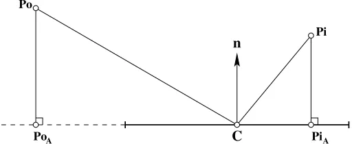
Point-Face. The closest point on a face (which is a polygon with an arbitrary number of sides) to an arbitrary 3D point,P, can either be a face vertex, lie on an edge, or lie on the face itself. Figure 9 shows these three cases. The question of whether the point is within rcut of the face can be determined by the

following algorithm. The structure of this point-face algorithm is such that it only evaluates as much of the problem as is necessary to make a decision about whether the point is in range of the face. Once it is has this, it stops the evaluation of the current point-face pair and moves on to the next.

(i) ProjectPto the nearest point,PA on the plane defined by the face centre,Cand normal unit vector,

A

Pi

A

Po

Pi Po

n

C

Figure 10. Projecting the point to be evaluated onto the plane defined by the face centre and normal unit vector. The projected point can either lie outside (Po_A) or inside (Pi_A) the face.

PA =P−((P−C)·n)n. (1)

If|(P−C)·n|> rcutthen it is not possible for the point to be in range of the face1. No more calculation is necessary for this pair.

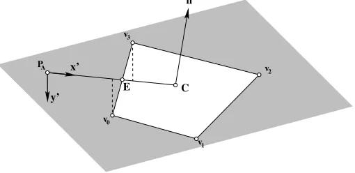
(ii) Whether PA lies inside or outside of the face must be determined. A line PAC is drawn fromPA to

C, along the plane of the face and each edge of the face is tested to see if this line crosses it. To do this, all of the vertices, v0,v1. . .vN, are projected onto a local 2D coordinate system that coincides with the plane of the face, withPA as its origin, see figure 11. This is necessary because PACand an edge may be skew if considered as 3D lines due to numerical round-off errors in the description points of the face, or where a face is not perfectly flat [17]. The axis unit vectors of the coordinate system on the plane are

x′= C−PA

|C−PA|, (2)

y′= (C−PA)×n

|(C−PA)×n|, (3)

(4)

and the position vector of a vertex, vα, in plane coordinates is

v′α = (vα−PA)·x′

x′+ (vα−PA)·y′

y′. (5)

Given that Clies on the line of x′_{, by definition}

C′=|C−PA|x′. (6)

When determining the local coordinates of the vertices, if |P−vα| ≤ rcut then the face must be in

range of the point. No more calculation is necessary for this pair.

(iii) Finding E, the intersection point between PAC and the edge defined by vertices v′α and v′β. The

equations forE′ _{(the intersection in plane coordinates) on the lines P}′

AC′ and v′αv′β are

1

The test actually performed is|(P₋C_)·n_|2_{> r}2

cutto avoid the square root when determining the magnitude of the vector. All

v0

v3

v1

v2

PA

y’ E C

x’

n

Figure 11. Defining a coordinate system local to the plane of the face to calculate intersections with face edges.

E′=λAC′, (7)

E′=v′α+λv v′β−v′α. (8)

Expanding equations (7) and (8) in x′ and y′ components

E_x′′ =λAC_x′′,

E_y′′ =λAC_y′′,

E_x′′ =v_αx′ ′ +λv v_βx′ ′ −v′_αx′

,

E_y′′ =v_αy′ ′+λv v′_βy′ −v_αy′ ′

,

and solving forλAand λv, given thatC_y′′ = 0 becauseE′ lies on the line of x′

λA= 1

C_x′′



v_αx′ ′ −v′_αy′

v′

βx′ −v′_αx′

v_βy′ ′ −v

′ αy′



, (9)

λv =− v′

αy′

v′

βy′−v_αy′ ′

. (10)

If 0≤λA≤1 and 0≤λv ≤1, then the edge in question is crossed betweenPA andC.PA must have

been outside of the face, and E is the closest point on the face toP,

E=PA+λA(C−PA). (11)

If |P−E| ≤rcut then the face is in range of the point. If no edge is crossed byPAC, then PA must

have been on the face, so if |PA−P| ≤rcut then the face is in range of the point, and the cells that the face forms part of must interact with the cells that the point forms part of.

c₁ c₂ v_α

v_β v_γ

v_δ

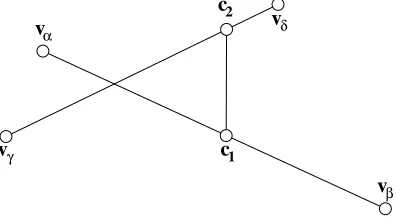
Figure 12. The closest distance between two edges.

Edge-Edge. Using the derivation of the closest distance between two skew lines [27] to determine whether two edges are within range of each other. The equations for the closest points on the lines that the edges to be compared lie on, see figure 12, are

c1 =vα+λ1(vβ−vα), (12)

c2=vγ+λ2(vδ−vγ). (13)

Defining [28],

a=vβ−vα,

b=vδ−vγ,

c=vγ−vα,

and solving equations (12) and (13) forλ1 and λ2 gives

λ1=

(c×b)·(a×b)

|a×b|2 , (14)

λ2= (c×a)·(a×b)

|a×b|2 . (15)

If|a×b|= 0, then the lines are parallel and this algorithm is invalid. A point-face search will, however, identify parallel edges as being in range if necessary. No more calculation is necessary for this edge pair.

If 0≤λ1 ≤1 and 0≤λ2≤1, then the closest points between the lines lie somewhere along both edges.

In this case, calculate c1 and c2 using equations (12) and (13) and test |c1−c2| ≤ rcut to determine if

the edges, hence the cells they form part of, are in range. Edge-edge searching is reciprocal and can be performed under a non-double-counting loop.

2.4 Intermolecular Force Calculation Procedure

2.4.2 Build Cell Occupancy and Refer Molecules. At each timestep, before calculating any forces, a list for each cell is built stating which molecules it contains. This is a computationally cheap operation because it only involves querying each molecule for which cell it is in, and adding a reference or pointer to that molecule to the list for the appropriate cell. Each molecule holds information about which cell it occupies by virtue of the tracking mechanism [17].

At each timestep, all real cells which are the source cell of one or more referred cells send the position and id of all of the molecules they contain to the appropriate referred cell on the appropriate processor. The destination referred cells perform the appropriate position and orientation transformation when the molecules are received. The referred molecules are discarded and re-created from the source molecules at each timestep.

2.4.3 Force Calculation. The total intermolecular force acting on a molecule is calculated at each timestep by considering two types of interactions. Real-Real interactions occur between a molecule and others on the same processor, according to algorithm 2. Real-Referred interactions occur between real molecules and referred molecules arising from the other side of a processor or periodic boundary, according to algorithm3. Referred molecules do not need to calculate interactions between themselves, because every referred molecule is a copy of a real molecule elsewhere, and as such will receive all of its real-real and real-referred interactions in-situ.

Algorithm 2Real-Real Molecule Force Calculation.

forall real cells, ci do

for all real molecules inci,mi do forall real cells inci’s DIL,cj do

for all real molecules incj,mj do

calculate intermolecular forcefij between mi and mj

addfij to fi (total force vector formi)

addfji =−fij to fj

end for end for

forall real molecules in ci with an index greater than mi,mi′∗ do calculate intermolecular force fii′ between mi and mi′

add fii′ to f_i add −fii′ to f_i′

end for end for end for

∗_{Comparison of the index of molecules in the same cell,m}′

I > mI, means that interactions between molecules in the same cell are

not double-counted and a molecule does not calculate an interaction with itself. The order of comparison is not important, as long as all pairs are covered, som′

I< mI would work equally well.

Algorithm 3Real-Referred Molecule Force Calculation

forall referred cells, cq do

for all referred molecules incq,mq do

forall real cells that cq interacts with, cp do

for all real molecules incp,mp do

calculate intermolecular forcefpq between mp and mq

addfpq to fp

3 Implementation and Performance

3.1 gnemdFOAM

AICA has been implemented in OpenFOAM [16], which is an open source C++ library intended for continuum mechanics simulation of user-defined physics (primarily used for CFD) in arbitrary, unstruc-tured geometries. The AICA MD code has been built using OpenFOAM’s lagrangian particle tracking library [17] and is called gnemdFOAM. All features of OpenFOAM have a common infrastructure for distributed memory parallel processing using MPI.

3.2 Accuracy: Single Timestep Average Pair Potential Energy

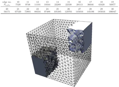
The total potential energy of all pair interactions in a test system was calculated by an in-house code, gnemd, which was based on, and is validated against, the code supplied in [18]. The positions of all of the molecules from the gnemd test case were imported into gnemdFOAM, transferring with a precision of 18 decimal places. The same system (same bounding box geometry and same intermolecular potential) was simulated by gnemdFOAM using a regular cubic mesh and 21 different tetrahedral meshes generated by commercial CFD meshing software GAMBITR. The cubic mesh ingnemdFOAM comprised 283 = 21952 cubic cells. The tetrahedral meshes were generated by specifying the number of cell edges to be placed on the edges of the bounding geometry, and allowing GAMBITRto automatically generate a tetrahedral mesh. Edge numbers of 10–30 were used and the number of cells generated in each case shown in table 1. An example mesh (edge number 15) is shown in figure 13.

All MD values in these tests will be expressed in reduced units scaled using the Argon Lennard Jones (LJ) potential length, energy and mass values. The shifted-force [19] LJ intermolecular potential for Argon withrcut= 2.5 was used in all simulations:

u(rij) =



    

    

4ǫ

σ rij

12

−_rσ ij

6

−

σ rcut

12

−_rσ cut

6

+ 12rcut(rij−rcut)

σ2

σ rcut

14

−1_2rσ cut

8

, rij ≤rcut

0, rij > rcut.

(16)

A cubic system domain of exactly 50 units side length was chosen to avoid any round-off errors when generating the mesh geometry, and a fluid number density of (50/46)−3= 0.778688 chosen to give a perfect simple cubic lattice of 463 = 97336 molecules. The total potential energy of all pair interactions for the molecules in their initial configuration, divided by the number of molecules, will be used to compare the results. This average potential per molecule, hP Ei, was calculated using gnemd, hP Eig, and by

gnemd-FOAM for 22 meshes (21 tetrahedral and cubic) using the PP, PPGR (withrG= 0.125,0.25,0.5,1.0) and PFEE cell interaction identification methods. The cubic mesh ingnemdFOAM was not sensitive to any of the mesh searching errors of PP identified in section 2.3.1 and produced exactly the same result,hP EigF,

with each of the cell interaction identification methods:

hP Eig =−4.22656275761469,

hP EigF =−4.22656275759921,

hP Eig− hP EigF

hP EigF

= 3.64×10−12. (17)

The difference betweenhP Eig and hP EigF, equation (17), is thought to arise from the accumulation of

Table 1. Number of cells in test tetrahedral meshes generated by GAMBIT.R

edge no. 10 11 12 13 14 15 16 17 18 19

Ncells 7520 9748 11101 19344 22289 22338 28113 36646 43420 50877

20 21 22 23 24 25 26 27 28 29 30

56171 67520 73801 88334 97488 105385 129761 145016 145196 185016 196847

Figure 13. Tetrahedral mesh with edge number 15. The outline of cells on four of six faces of the bounding cube are shown and two of twelve portions of cells are shown from the mesh decomposed for parallelisation.

10-13 10-12 10-11 10-10 10-9 10-8 10-7 10-6 10-5 10-4 10-3

0 40000 80000 120000 160000 200000

Relative error magnitude

Number of cells

PP

PPGR, r_G = 0.125 PPGR, r_G = 0.25 PPGR, r_G = 0.5 PPGR, r_G = 1 PFEE

g to gF, cubic mesh

10-14 10-13 10-12 10-11 10-10

0 40000 80000 120000 160000 200000

Relative error magnitude

Number of cells

12 processor PFEE, parallel to serial error 32 processor PFEE, parallel to serial error 12 processor PFEE, parallel self error 32 processor PFEE, parallel self error

Figure 15. Relative error inhP Eifor each tetrahedral mesh simulated in parallel using 12 and 32 processors. Cell interactions built with PFEE.

relative error between hP Ei for the tetrahedral meshes using the various cell interaction methods and hP EigF is calculated in the same manner as equation (17) and shown in figure 14. The errors in the PP or

PPGR results are due to cells containing molecules that should interact not being identified by point-point searching of the mesh. The errors in PP and PPGR simulations become smaller in meshes with more cells because a fixed rcut+rG length becomes larger relative to the cell size, giving a greater chance of

establishing two points of a cell being in range.

Note that PFEE always produces a result that appears to be on the numerical ‘noise floor’ of the simu-lation — where the cumulative effect of numerical rounding errors becomes important. This is supported by the PPGR results dropping onto this line whenrGis large enough, indicating that all errors have been

removed. This line has a smaller magnitude than the value from equation (17), which is plotted as ‘g to gF, cubic mesh’. This demonstrates that PFEE identifies the correct cells to provide every molecular interaction in the system, irrespective of mesh topology.

3.2.1 Parallel Accuracy. The accuracy of PFEE when the simulation is parallelised is demonstrated in figure 15. The tetrahedral meshes were decomposed into 12 portions (as shown in figure 13) by a simple

x:y :z = 2 : 3 : 2 split and into 32 portions using METIS [29], then simulated on a distributed memory parallel cluster. The ‘parallel to serial error’ data represents the relative difference betweenhP Eicalculated for each mesh andhP EigF. The ‘parallel self error’ data represents the difference betweenhP Eicalculated

10-3 10-2 10-1 100 101

0 0.02 0.04 0.06 0.08 0.1

Probability

Relative acceleration error magnitude PP

PPGR, r_G = 0.125 PPGR, r_G = 0.25 PPGR, r_G = 0.5 PPGR, r_G = 1 10-3

10-2

0.1 0.15 0.2 0.25 0.3 0.35

Figure 16. Relative error magnitude distribution for tetrahedral mesh, edge number 14.

3.2.2 Distribution of Errors. The values of hP Eifor PP and PPGR do not give an indication of how the intermolecular force errors due to missed interactions are distributed. If a large number of molecules experience small errors, then this is perhaps tolerable. If, however, a small number of molecules receive substantial errors, this will may cause unacceptable perturbations to the dynamics. The latter case is observed in practice.

The system simulated above is initialised in the cubic mesh with molecule velocities drawn from a Maxwellian distribution at a temperature of 2.5 and allowed to evolve in gnemdFOAM using the Verlet leapfrog [18] integration scheme for 1000 timesteps of ∆t= 0.005 to create a reference system. This was done to let the initial simple cubic lattice relax into a more realistic configuration, because the net force on each molecule in the perfect crystal is zero, which is not useful for calculating relative errors. The molecule positions from the reference system are used in the tetrahedral meshes and the acceleration vector for each molecule calculated. The absolute and relative error magnitude between the acceleration for each molecule in the tetrahedral mesh and the acceleration for the corresponding molecule in the reference system is calculated:

absolutei=|ateti−arefi|, (18)

relativei=

|atet_i−aref_i| |arefi|

. (19)

These errors were added to histograms to assess their distribution. Examples of the histograms are shown in figures 16 and 17 for the edge number 14 mesh, using PP and PPGR (rG = 0.125,0.25,0.5,1.0). Both

10-5 10-4 10-3 10-2 10-1 100

0 0.5 1 1.5 2 2.5

Probability

Absolute acceleration error magnitude PP

PPGR, r_G = 0.125 PPGR, r_G = 0.25 PPGR, r_G = 0.5 PPGR, r_G = 1

Figure 17. Absolute error magnitude distribution for tetrahedral mesh, edge number 14.

3.3 Computational Speed

The computational speed of establishing cell interactions and calculating intermolecular forces in gnemd-FOAM was assessed for each of the tetrahedral meshes above, filled with 97336 LJ molecules. The time taken to build the interaction lists (create DILs, create referred cells and find real cells in range of referred cells) was recorded, and an intermolecular force calculation for all molecules performed 400 times and timed. The molecules were not moved during the simulation. All timing tests were performed on a PC with a 2.8GHz, AMD AthlonTM_{FX-62 processor.}

The time taken to build the interaction lists is shown in figure 18 (note the logarithmic time axis). For the PP and PPGR data, an increase with increasing rG is seen because more referred cells will be

created. It is clear that PFEE takes substantially longer than PP or PPGR to build the interaction lists. This is understandable given the number of comparisons and calculations required by PFEE. Building the interaction lists is O(N2), for a mesh of N cells, and as such benefits greatly from parallelisation because each portion of the mesh only needs to search itself. The longest PFEE builds, taking several 1000s of seconds, would typically not be practical and the mesh would be decomposed and the simulation parallelised. The interaction lists are established only once, at the start of the simulation, so for a very long simulation this may not represent a substantial portion of the total time. If the same mesh with the same

rcut is to be used repeatedly, then the cell interaction information can be calculated once then written to and read from disk.

The average time taken per timestep to calculate the intermolecular forces is shown on figure 19. All of the results follow a similar trend: in meshes with few cells, each cell contains a large number of molecules, and many pairs identified to interact will be further apart than rcut. As the cells become smaller, the

1 10 100 1000 10000 100000

0 40000 80000 120000 160000 200000

Computational time to build interaction lists/[s]

Number of cells

PP PPGR, r_G = 0.125 PPGR, r_G = 0.25 PPGR, r_G = 0.5 PPGR, r_G = 1.0 PFEE

Figure 18. Time taken to build interaction lists at the start of the simulation.

The PP and PPGR results produce a family of curves, with increasing rG the computational time

increases and the region of the ‘dip’ narrows. An increased guard radius will produce DILs with unnecessary cells on them and unnecessary real-referred cell interactions, increasing the number of intermolecular evaluations between pairs of molecules that are further apart thanrcut.

The PFEE result has a similar form to PP and PPGR but does not fit into the family. In meshes with fewer cells, PFEE is more expensive than PP and most of the PPGR results because it is correctly identifying cells to interact that PP and PPGR miss. Comparing 19 to figure 14 it can be seen that the ‘dip’ (up to approximately 40000 cells) in computational time coincides with the region of maximum errors for PP and PPGR — missed cell interactions emphasise the ‘dip’ by reducing the number of calculations required by each molecule. The fact that PFEE does not take significantly longer to calculate forces than PP for larger meshes demonstrates that it does not identify any more cells to interact than are absolutely necessary.

There is a opportunity to trade-off the time taken to build the interaction lists using PFEE with a quick list build and slower timesteps using PPGR and a large enough rG to remove all errors. The required rG length is difficult to determine in advance, however, and most realistic simulations involve very many

timesteps, which would soon make the PPGR simulation slower overall.

Simulations to characterise the performance of the code, exploring the impact of number density, system size, mesh cell size and morphology (for example, tetrahedral vs. hexahedral, skew, aspect ratio) number of processors and decomposition method will be presented in a future publication.

4 Discussion and Conclusions

The AICA algorithm is able to identify cells which are within a distance rcut of each other in a mesh

1 1.5 2 2.5 3 3.5

0 40000 80000 120000 160000 200000

Computational time per timestep/[s]

Number of cells

PP PPGR, r_G = 0.125 PPGR, r_G = 0.25 PPGR, r_G = 0.5 PPGR, r_G = 1.0 PFEE

Figure 19. Time taken to calculate intermolecular pair forces between all molecules.

Edge-Edge (PFEE) searching of the mesh.

The accuracy of using PFEE mesh searching to determine which cells in the mesh should interact has been demonstrated by simulating a cubic MD system represented by 21 different tetrahedral meshes, ranging from 7520 to 196847 cells. The results are the same, to within numerical round off error, to those produced by another verified MD code. The computational cost of intermolecular force calculation with AICA depends on the mesh used (see below) but scales favourably with increasing refinement of the mesh. In particular, having a significant number of empty cells does not add much computational overhead. The accuracy of exchanging intermolecular force data across periodic and interprocessor boundaries using referred molecules and cells has been demonstrated, with the 21 tetrahedral meshes producing the same results when simulated in serial as on 12 and 32 processors.

4.1 Choosing a Mesh

The performance of the algorithm is highly dependent on the mesh it is applied to. When choosing a mesh to use for a simulation the following points must be considered, and in some cases numerically tested and traded-off against one another:

• The time required to build cell interaction lists depends on the intermolecular potential cut-off radius,

rcut, the number of cells and their shape, and the form of the mesh: a tetrahedral mesh will have a

difference balance of points:edges:cells compared to a hexahedral mesh, which will impact on the time taken for a PFEE search.

• Optimising the size of the mesh to minimise the time taken to run the simulation is complex and is case-specific, as demonstrated in section 3.3.

• The mesh is not only used to define the shape of the domian and to help identify interacting molecules, thermodynamical and fluid mechanical fields are spatially resolved onto it and the mesh resolution may be dictated by this.

‘tricks of the trade’ used in CFD can also be applied, for example the mesh can be adaptively refined to track a region of interest.

• The results in section 3 showed that PP and PPGR are generally not good choices for building cell interactions unless either the mesh in question comprises fairly regular hexahedra or some errors can be tolerated.

4.2 Future Developments

Currently this algorithm deals only with short-ranged pair forces. Future developments will incorporate rigid and flexible polyatomic molecules, and long-range electrostatic forces. A hybrid MD/continuum implementation in OpenFOAM is currently under development. OpenFOAM is ideal for incorporating polar fluids and electrokinetic actuation, which feature in envisioned applications, because it is able to simulate electromagnetic, magnetohydrodynamic and fluid mechanic continuum fields on the same mesh that AICA operates on.

5 Acknowledgements

The authors would like to thank Chris Greenshields and Matthew Borg of Strathclyde University, and Henry Weller and Mattijs Janssens of OpenCFD Ltd. for useful discussions. This work is funded in the UK by Strathclyde University, the Miller Foundation and the James Weir Foundation, and through a Philip Leverhulme Prize for JMR from the Leverhulme Trust.

References

[1] Peter Agre. The aquaporin water channels. Proceedings of the American Thoracic Society, 3(1):5–13, 2006.

[2] Joel Koplik and Jayanth R. Banavar. Continuum deductions from molecular hydrodynamics.Annual Review of Fluid Mechanics, 27:257–292, 1995.

[3] H. Brenner and V. Ganesan. Molecular wall effects: are conditions at a boundary “boundary condi-tions”? Physical Review E, 61(6):6879–6897, 2000.

[4] D. Hirshfeld and D.C. Rapaport. Molecular dynamics simulation of Taylor-Couette vortex formation. Physical Review Letters, 80(24):5337–5340, 1998.

[5] D.C. Rapaport and E. Clementi. Eddy formation in obstructed fluid flow: a molecular-dynamics study. Physical Review Letters, 57(6):695–698, 1986.

[6] K.P. Travis, B.D. Todd, and D.J. Evans. Poiseuille flow of molecular fluids. Physica A, 240(1-2):315– 27, 1997.

[7] K.P. Travis, B.D. Todd, and D.J. Evans. Departure from Navier-Stokes hydrodynamics in confined liquids. Physical Review E, 55(4):4288–95, 1997.

[8] Tiezheng Qian and Xiao-Ping Wang. Driven cavity flow: from molecular dynamics to continuum hydrodynamics. Multiscale Modeling and Simulation, 3(4):749–763, 2005.

[9] Thomas Becker and Frieder Mugele. Nanofluidics: viscous dissipation in layered liquid films. Physical Review Letters, 91(16):166104, 2003.

[10] Hisashi Okumura and David M. Heyes. Comparisons between molecular dynamics and hydrodynamics treatment of nonstationary thermal processes in a liquid. Physical Review E, 70(6):061206, 2004. [11] Rafael Delgado-Buscalioni and Peter V. Coveney. Hybrid molecular-continuum fluid dynamics.

Philo-sophical Transactions of the Royal Society London, 362(1821):1639–1654, 2004.

[12] G. Wagner and E. G. Flekkøy. Hybrid computations with flux exchange. Philosophical Transactions of the Royal Society London, 362(1821):1655–1665, 2004.

[14] Thomas Werder, Jens H. Walther, and Petros Koumoutsakos. Hybrid atomistic-continuum method for the simulation of dense fluid flows. Journal of Computational Physics, 205(1):373–390, 2005. [15] Sumita Pennathur and Juan G. Santiago. Electrokinetic transport in nanochannels. 2. experiments.

Analytical Chemistry, 77(21):6782–6789, 2005.

[16] OpenFOAM: The Open Source CFD Toolbox. http://www.openfoam.org.

[17] Graham B. Macpherson, Niklas Nordin, and Henry G. Weller. Particle tracking in unstructured, arbitrary polyhedral meshes for use in CFD and molecular dynamics. Submitted to Communications in Numerical Methods in Engineering. Preprint included in submission for review, 2007.

[18] D. C. Rapaport. The Art of Molecular Dynamics Simulation. Cambridge University Press, 2nd edition, 2004.

[19] M.P. Allen and D.J. Tildesley. Computer simulation of liquids. Oxford University Press, 1987. [20] W. Smith. Molecular dynamics on hypercube parallel computers.Computer Physics Communications,

62(2–3):229–248, 1991.

[21] D.C. Rapaport. Multi-million particle molecular dynamics. II. Design considerations for distributed processing. Computer Physics Communications, 62(2–3):217–228, 1991.

[22] Tim N. Heinz and Philippe H. Hunenberger. A fast pairlist-construction algorithm for molecular simulations under periodic boundary conditions. Journal of Computational Chemistry, 25(12):1474 – 1486, 2004.

[23] W. Mattson and B.M. Rice. Near-neighbor calculations using a modified cell-linked list method. Computer Physics Communications, 119(2-3):135 – 48, 199.

[24] Pedro Gonnet. A simple algorithm to accelerate the computation of non-bonded interactions in cell-based molecular dynamics simulations. Journal of Computational Chemistry, 28(2):570–573, 2007. [25] Cgal_{, Computational Geometry Algorithms Library. http://www.cgal.org.}

[26] Kaspar Fischer, Bernd Grtner, Thomas Herrmann, Michael Hoffmann, Sven Schnherr, and the CGAL Editorial Board. Optimal distances. In CGAL User and Reference Manual. 3.3 edition, 2007. [27] W. Gellert, S. Gottwald, M. Hellwich, H.; K¨astner, and H. K¨unstner, editors. VNR concise

encyclo-pedia of mathematics. Van Nostrand Reinhold, New York, 2nd edition, 1989.

[28] Eric W Weisstein. Line-line distance. From MathWorld — A Wolfram Web Resource. http://mathworld.wolfram.com/Line-LineDistance.html.

Appendix A: Neighbour List Lifetime Prediction

The computational cost of the neighbour list algorithm depends on the number of timesteps a neighbour list remains valid for — a quantity whose dependence on simulation properties can be predicted. For a given number of molecules, N, of mass m, in equilibrium at a temperature T, there is a probability of 1/N that a molecule in the system will be travelling with a velocity vN. It is therefore likely that at every

timestep there will beone molecule travelling at, or close to this velocity. Given that a neighbour list is invalidated when the cumulative sum ofmaximum displacements in the system exceeds a fixed threshold (usually 0.5∆R, half the shell thickness [18]), finding the number of timesteps required for a molecule travelling at vN to cover this distance gives an estimate of the lifetime of the list. Estimating vN by

equating the Maxwellian velocity distribution to 1/N, where T,m and vN are in reduced MD units [19]

(see figure A1):

4π m

2πT

32

v2_Ne

„

−mv2_N

2T

«

= 1

N. (A1)

The high speed solution is,

vN(T, m, N) =

v u u t−

2T

mW−1 −

1 4N

r

2πT m

!

, (A2)

whereW−1 is the secondary real branch of the Lambert W function.

The accuracy ofvN as a prediction of the maximum velocity in the system has been tested experimentally.

Two systems containing 1728 and 13824 Lennard-Jones molecules,m= 1, at a number density of 0.8 were equilibrated to two different temperatures, T = 1.0 and T = 2.5, then simulated for 44000 timesteps of ∆t= 0.005. At each timestep the maximum velocity in the system was found and added to a histogram with a velocity bin width of 0.05. The histograms were then normalised to produce probability functions, their mean calculated, and the data was fitted to a curve of the form,

fvN(x) =p(x−s)

q_e−(x−s)/r_{. (A3)}

Figure A2 shows the maximum velocity probability functions with their mean and the corresponding value ofvN(T, m, N). Table A1 shows the pertinent data and the curve fitting parameters for each result.

The values ofvN and the distribution mean are close in all four cases, withvN consistently higher (2-5%

– 5.5% in these examples) but lying comfortably within the distribution. UsingvN will probably result in

a slightly pessimistic estimate of the lifetime of a neighbour list.

The number of timesteps (of length ∆t) a neighbour list is valid for, L, is given by

L=

0.5∆R

∆tvN

. (A4)

This lifetime reduces with increasing temperature and number of molecules, as shown in figure A3, resulting in a higher computational cost when using neighbour lists. At higher temperatures,vN is higher because

the velocity distribution covers a higher molecular speed range. In systems comprising more molecules, it is more probable that at least one molecule will be travelling at a given speed in the upper region of the distribution, therefore vN is also higher. The cost of an algorithm such as AICA, based only on cell

Probability

Velocity Magnitude 1/N

v_N

Figure A1. Maxwellian velocity distribution. Finding velocities corresponding to a probability of 1/N, whereNis the number of molecules in the system. There are two real, positive solutions — the high speed one isvN, the quantity of interest.

Table A1. Experimental data and curve fitting parameters forf_vN(x).

T N vN mean vN− mean

mean p q r s

1 1728 4.528 4.294 5.45% 17310 6.794 0.1008 3.504 1 13824 5.006 4.783 4.66% 47060 7.027 0.08975 4.058 2.5 1728 6.979 6.821 2.31% 610.7 8.334 0.1494 5.416 2.5 13824 7.756 7.558 2.62% 1276 7.157 0.1406 6.406

0 0.2 0.4 0.6 0.8 1 1.2 1.4 1.6 1.8

3 3.5 4 4.5 5 5.5 6 6.5

probability

Maximum velocity in timestep (reduced units) T = 1, m = 1

N = 13824: mean = 4.783 v_N(1,1,13824) = 5.006 N = 1728: mean = 4.294

v_N(1,1,1728) = 4.528

N = 13824: data N = 13824: fit N = 1728: data N = 1728: fit

0 0.2 0.4 0.6 0.8 1 1.2

5 6 7 8 9 10

probability

Maximum velocity in timestep (reduced units) T = 2.5, m = 1

N = 13824: mean = 7.558 v_N(2.5,1,13824) = 7.756 N = 1728: mean = 6.821

v_N(2.5,1,1728) = 6.979

N = 13824: data N = 13824: fit N = 1728: data N = 1728: fit

Figure A2. Probability of maximum velocity in simulation atT= 1.0 (left) andT = 2.5, (right) for 1728 and 13824 Lennard-Jones molecules of massm= 1 compared tovN(T, m, N). The data was collected from 44000 timesteps of ∆t= 0.005. The mean of the

distributions is shown for comparison. Temperature, velocity and mass are expressed in reduced units.

equation (A4) reduces the impact of the difference between vN and the measured mean of the maximum

4 5 6 7 8 9 10 11 12

102 103 104 105 106

Predicted number of timesteps of neighbourList validity

Number of molecules, N (m = 1, ∆R = 0.4, ∆t = 0.005) T = 1 T = 1.5 T = 2.5

Figure A3. Variation of estimated neighbour list lifetime with typical simulation parameters for a Lennard Jones fluid [18].T, m,∆R

and ∆tare in reduced MD units.

Appendix B: Build Cell Interactions

Building DILs, creating referred cells and determining which real cells are in range of them is allowed to be computationally expensive (within reason) because it will only happen once at the beginning of the MD simulation, if the mesh is static. Accessing the information, however, must be as fast as possible because it will happen at every timestep. In each of these steps either the PP, PPGR or PFEE method can be used to test whether or not two cells are withinrcutof each other.

B.1 Building DILs

The construction of the DILs and accessing molecules is done in such a way as to not double-count interactions. For example, if cells A and B need to interact, cell B will be on cell A’s DIL, but cell A will not be on cell B’s DIL. When a molecule in cell A interacts with one in cell B the molecule in cell B will receive the inverse of the force vector calculated to be added to the molecule in cell A, because the pair forces are reciprocal, i.e.fab=−fba.

When using PP or PPGR, all points in the mesh are compared, as per algorithm 1. When two points are in range, this produces a set of cells attached to one point and another set attached to the other point. When using PFEE, all points are compared to all faces. When this pair are in range the set of cells that are attached to the point and the set of cells that the face forms part of are produced. All edges in the mesh are compared in a non-double-counting loop, and when they are in range two sets of cells are again produced — those attched to one edge and those attached to the other.

For each step in each method, two sets of cells are returned. The index of each cell in one set is compared to the index of each cell in the other set, and the cell with the higher index is added to the DIL of the cell with the lower index. Cells are not added to their own DIL.

B.2 Creating Referred Cells

Coupled patches are the basis of periodic and interprocessor communication for creating referred cells. Patches, in general, are an OpenFOAM class comprising a collection of cell faces representing a mesh boundary of some description — they may provide solid surfaces, inlets, outlets, symmetry planes, periodic planes, or interprocessor connections. Coupled patches provide two surfaces; that which exits one enters the other and vice versa. Two types are used in AICA:

coupled periodic surfaces. When a molecule crosses a face on one surface, it is wrapped around to the corresponding position on the corresponding face on the other surface.

• Processor patches provide links between portions of the mesh on different processors, one half of the patch is on each processor. When a molecule crosses a face on one surface, it is moved to the corresponding position on the corresponding face on the other surface, on the other processor. Decomposing a mesh for parallelisation will often require a periodic patch to be changed to a processor patch.

The surfaces of coupled patches may have any relative orientation, and may be spatially separated as long as the face pairs on each surface correspond to each other.

B.2.1 Create Patch Segments. In the decomposed portion of the mesh on each processor, each processor and periodic patch should be split into segments, such that:

• faces on a processor that were internal to the mesh prior to decomposition end up on a segment; • faces on a processor patch that were on separate periodic patches on the undecomposed mesh end up

on different segments. These segments are further split such that faces that were on different halves of the periodic patch on the undecomposed mesh end up on different segments;

• faces on different halves of a periodic patch end up on different segments.

Each segment must produce a single vector/tensor transformation pair (see appendix C) which will be applied to all cells referred across it.

B.2.2 Cell Referring Iterations. For each patch segment:

(i) Find all real and existing referred cells with a portion of their surface in range of the faces comprising the patch segment.

(ii) Refer or re-refer this set of cells across the boundary defined by the patch segment using its trans-formation, see appendix C. In the case of a segment of periodic boundary, this creates new referred cells on the same processor. For a segment of a processor patch, these cells are communicated to, and created on the neighbouring processor. Before creating any new referred cell a check is carried out to ensure that it is not

• a duplicate referred cell, one that has been created already by being referred across a different segment;

• a referred cell trying to be duplicated on top of a real cell, i.e. a cell being referred back on top of itself.

If the proposed cell for referral would create a duplicate of an existing referred cell, or end up on top of a real cell, then it is not created. To be a duplicate, the source processor, source cell and the vector part of the transformation (see appendix C) must be the same for the two cells (note, the vector part of transformation for a real cell is zero by definition).

A single run of these steps will usually not produce all of the required referred cells. They are repeated until no processor adds a referred cell in a complete evaluation of all segments, meaning all possible interactions are accounted for. In iterations after the first, in step 1 it is enough to search only for referred cells in range of the faces on the patch segment, because the real cells will not have changed and would all be duplicates. The final configuration of referred cells does not depend on the order of patch segment evaluation.

B.3 Determining Real Cells in Range of Referred Cells

Processor 2 Processor 1

Processor 0

Figure B1. An arbitrary unstructured mesh, which is periodic top-bottom and left-right. It is decomposed into 3 irregular portions for parallel processing as marked.

with. This process is accelerated by only searching a subset of the real cells in the mesh. These are the real cells that were identified as being in range of any processor or periodic patch when creating the referred cells. This set is guaranteed to contain all cells that could be in range of a referred cell.

B.4 Example Construction of Referred Cells

Figures B1 and B2 show the start and end points of the cell referring operation on a mesh that has been decomposed to run in parallel. The example is in 2D for clarity but the process is exactly the same in 3D. In this example the number of referred cells created exceeds the number of real cells, which would lead to much costly interprocessor communication. This is because the mesh has been made deliberately small relative torcutto demonstrate as many features of the algorithm as possible and to be practical to

understand. In realistic systems, the mesh portions would be significantly bigger thanrcutand the referred

Referred cell Source on processor 0

Referred cell Source on processor 1

Referred cell Source on processor 2

00000 00000 00000 00000 00000 11111 11111 11111 11111 11111 Real cell 000 000 000 000 000 000 111 111 111 111 111 111 000000 000000 000000 000000 111111 111111 111111 111111 000000 000000 000000 000000 111111 111111 111111 111111 0000 0000 0000 0000 0000 0000 1111 1111 1111 1111 1111 1111 00000 00000 00000 00000 11111 11111 11111 11111 00000 00000 00000 00000 00000 00000 11111 11111 11111 11111 11111 11111 0000 0000 0000 0000 0000 0000 0000 1111 1111 1111 1111 1111 1111 1111 0000 0000 0000 0000 0000 1111 1111 1111 1111 1111 0000 0000 0000 0000 0000 1111 1111 1111 1111 1111 0000 0000 0000 0000 0000 0000 0000 1111 1111 1111 1111 1111 1111 1111 0000 0000 0000 0000 0000 0000 0000 1111 1111 1111 1111 1111 1111 1111 0000 0000 0000 0000 0000 1111 1111 1111 1111 1111 00000 00000 00000 00000 11111 11111 11111 11111 000 000 000 000 111 111 111 111 000 000 000 000 111 111 111 111 00000 00000 00000 00000 00000 11111 11111 11111 11111 11111 0000 0000 0000 0000 1111 1111 1111 1111 00000 00000 00000 11111 11111 11111 0000 0000 0000 0000 0000 1111 1111 1111 1111 1111 00000 00000 00000 00000 11111 11111 11111 11111 0000 0000 0000 0000 0000 1111 1111 1111 1111 1111 0000 0000 0000 0000 0000 1111 1111 1111 1111 1111 0000 0000 0000 0000 1111 1111 1111 1111 0000 0000 0000 0000 1111 1111 1111 1111 0000 0000 0000 0000 0000 1111 1111 1111 1111 1111 0000 0000 0000 0000 0000 1111 1111 1111 1111 1111 0000 0000 0000 0000 1111 1111 1111 1111 0000 0000 0000 0000 0000 1111 1111 1111 1111 1111 00000 00000 00000 00000 00000 11111 11111 11111 11111 11111 0000 0000 0000 0000 1111 1111 1111 1111 00000 00000 00000 00000 00000 11111 11111 11111 11111 11111 00000 00000 00000 00000 00000 11111 11111 11111 11111 11111 00000 00000 00000 11111 11111 11111 00000 00000 00000 11111 11111 11111 000000 000000 000000 111111 111111 111111 0000 0000 0000 0000 0000 1111 1111 1111 1111 1111 00000 00000 00000 00000 11111 11111 11111 11111 000000 000000 000000 000000 111111 111111 111111 111111 0000 0000 0000 0000 0000 0000 1111 1111 1111 1111 1111 1111 00000 00000 00000 00000 00000 11111 11111 11111 11111 11111 00000 00000 00000 00000 11111 11111 11111 11111 0000 0000 0000 0000 0000 1111 1111 1111 1111 1111 0000 0000 0000 0000 0000 0000 1111 1111 1111 1111 1111 1111 000000 000000 000000 111111 111111 111111 0000 0000 0000 0000 0000 1111 1111 1111 1111 1111 00000 00000 00000 00000 00000 11111 11111 11111 11111 11111 00000 00000 00000 00000 00000 00000 11111 11111 11111 11111 11111 11111 00000 00000 00000 00000 00000 11111 11111 11111 11111 11111 0000 0000 0000 0000 0000 1111 1111 1111 1111 1111 000 000 000 000 000 000 111 111 111 111 111 111 00000 00000 00000 00000 00000 00000 11111 11111 11111 11111 11111 11111 00000 00000 00000 00000 11111 11111 11111 11111 000 000 000 000 000 111 111 111 111 111 0000 0000 0000 0000 0000 0000 0000 1111 1111 1111 1111 1111 1111 1111 00000 00000 00000 00000 00000 00000 11111 11111 11111 11111 11111 11111 0000 0000 0000 0000 0000 0000 0000 0000 1111 1111 1111 1111 1111 1111 1111 1111 0000 0000 0000 0000 0000 0000 0000 1111 1111 1111 1111 1111 1111 1111 Processor 2 0000 0000 0000 0000 0000 1111 1111 1111 1111 1111 0000 0000 0000 0000 0000 1111 1111 1111 1111 1111 000000 000000 000000 000000 111111 111111 111111 111111 0000 0000 0000 0000 0000 1111 1111 1111 1111 1111 000000 000000 000000 111111 111111 111111 0000 0000 0000 0000 0000 1111 1111 1111 1111 1111 000000 000000 000000 111111 111111 111111 00000 00000 00000 00000 00000 11111 11111 11111 11111 11111 00000 00000 00000 00000 11111 11111 11111 11111 00000 00000 00000 00000 11111 11111 11111 11111 000000 000000 000000 000000 111111 111111 111111 111111 00000 00000 00000 00000 00000 00000 11111 11111 11111 11111 11111 11111 000 000 000 000 000 111 111 111 111 111 000000 000000 000000 000000 000000 111111 111111 111111 111111 111111 000000 000000 000000 000000 000000 000000 111111 111111 111111 111111 111111 111111 0000 0000 0000 0000 1111 1111 1111 1111 00000 00000 00000 00000 11111 11111 11111 11111 00000 00000 00000 00000 00000 11111 11111 11111 11111 11111 0000 0000 0000 0000 1111 1111 1111 1111 0000 0000 0000 0000 0000 1111 1111 1111 1111 1111 00000 00000 00000 00000 00000 11111 11111 11111 11111 11111 00000 00000 00000 00000 11111 11111 11111 11111 Processor 1 0000 0000 0000 0000 0000 1111 1111 1111 1111 1111 00000 00000 00000 00000 11111 11111 11111 11111 0000 0000 0000 0000 0000 0000 1111 1111 1111 1111 1111 1111 000000 000000 000000 111111 111111 111111 0000 0000 0000 0000 0000 0000 1111 1111 1111 1111 1111 1111 00000 00000 00000 00000 00000 11111 11111 11111 11111 11111 000000 000000 000000 111111 111111 111111 0000 0000 0000 0000 0000 1111 1111 1111 1111 1111 000000 000000 000000 111111 111111 111111 00000 00000 00000 00000 11111 11111 11111 11111 00000 00000 00000 00000 11111 11111 11111 11111 00000 00000 00000 00000 11111 11111 11111 11111 0000 0000 0000 0000 0000 1111 1111 1111 1111 1111 00000 00000 00000 00000 00000 11111 11111 11111 11111 11111 00000 00000 00000 00000 00000 11111 11111 11111 11111 11111 00000 00000 00000 00000 00000 11111 11111 11111 11111 11111 0000 0000 0000 0000 0000 1111 1111 1111 1111 1111 0000 0000 0000 0000 1111 1111 1111 1111 000 000 000 000 111 111 111 111 0000 0000 0000 0000 0000 1111 1111 1111 1111 1111 0000 0000 0000 0000 1111 1111 1111

1111 ₀₀₀₀00000000

0000 0000 1111 1111 1111 1111 1111 0000 0000 0000 0000 1111 1111 1111 1111 0000 0000 0000 0000 1111 1111 1111 1111 0000 0000 0000 0000 0000 1111 1111 1111 1111 1111 000 000 000 000 111 111 111 111 0000 0000 0000 0000 1111 1111 1111 1111 00000 00000 00000 00000 00000 11111 11111 11111 11111 11111 00000 00000 00000 00000 00000 11111 11111 11111 11111 11111 00000 00000 00000 00000 00000 11111 11111 11111 11111 11111 0000 0000 0000 0000 0000 1111 1111 1111 1111 1111 0000 0000 0000 0000 0000 0000 1111 1111 1111 1111 1111 1111 000000 000000 000000 111111 111111 111111 0000 0000 0000 0000 0000 1111 1111 1111 1111 1111 000000 000000 000000 111111 111111 111111 000000 000000 000000 111111 111111 111111 00000 00000 00000 00000 11111 11111 11111 11111 0000 0000 0000 0000 1111 1111 1111 1111 00000 00000 00000 00000 00000 11111 11111 11111 11111 11111 0000 0000 0000 0000 0000 0000 1111 1111 1111 1111 1111 1111 0000 0000 0000 0000 0000 0000 1111 1111 1111 1111 1111 1111 0000 0000 0000 0000 0000 0000 0000 1111 1111 1111 1111 1111 1111 1111 000 000 000 000 000 111 111 111 111 111 0000 0000 0000 0000 0000 1111 1111 1111 1111 1111 0000 0000 0000 0000 1111 1111 1111 1111 0000 0000 0000 0000 0000 0000 1111 1111 1111 1111 1111 1111 0000 0000 0000 0000 1111 1111 1111 1111 0000 0000 0000 0000 0000 0000 1111 1111 1111 1111 1111 1111 0000 0000 0000 0000 0000 0000 1111 1111 1111 1111 1111 1111 0000 0000 0000 0000 0000 0000 0000 1111 1111 1111 1111 1111 1111 1111 00000 00000 00000 00000 11111 11111 11111 11111 00000 00000 00000 00000 00000 11111 11111 11111 11111 11111 0000 0000 0000 0000 1111 1111 1111 1111 Processor 0

Figure B2. The final configuration of referred cells around the portions of the mesh in figure B1 on each processor. A circle of radius ˆ

rcutdrawn from any part of a real cell would be fully encompassed by other real or referred cells, thereby providing all molecules in that

cell with the appropriate intermolecular interactions, either across a periodic boundary or from another processor. Note that many cells are referred several times; for example, the source cell marked with⋆on processor 2 is referred to processors 0 and 1 twice on each.

Appendix C: Cell Referring Transformations

A spatial transformation is required to refer a cell across a periodic or processor boundary. Figure C1 shows the most general case of a cell being referred across a separated, non-parallel boundary, where,

α0 _{= Cell with a face on one side of the boundary,}

β0 = Cell with a face on the other side of the boundary, coupled toα0,

α1 _{= Cell α}0 _{referred across the boundary,} C= Cell centre,

n = Face normal unit vector,

Sα0_β0 =C_β0−C_α0. Position shift fromC_α0 to C_β0, Rα0

β0 = Tensor required to rotate −n

α0 to n

β0, given by,

Rα0_β0 =−(n_α·n_β)I+ (1 +n_α·n_β)

nα×nβ

|nα×nβ|

2

+nαnβ−nβnα, (C1)

where I is the identity tensor. The absolute position, P′_{, of a molecule transformed across a boundary}

(with its containing cell) from its original position P is required. To derive the P→P′ transform, first the position ofPrelative to the centre of the coupled face on α0 _{is given by}