by J. M. SULLIVAN, S. K. WILSONand B. R. DUFFY (Department of Mathematics, University of Strathclyde,
Livingstone Tower, 26 Richmond Street, Glasgow G1 1XH, United Kingdom)
[Received 26th January 2007. Revise 7th September and 11th October 2007]
Summary
The lubrication approximation is used to obtain a complete description of the steady unidirectional flow of a thin rivulet of perfectly wetting fluid on an inclined substrate subject to a prescribed uniform longitudinal surface shear stress. The quasi-steady stability of such a rivulet is analysed, and the conditions under which it is energetically favourable for such a rivulet to split into one or more subrivulets are determined.
1. Introduction
There are many practically important situations in which an external airflow has a significant effect on the behaviour of a film of fluid, and consequently a considerable amount of theoretical and numerical work has been undertaken in order to understand the flows that can occur. Examples include the work by King and Tuck (1) and King, Tuck and Vanden-Broeck (2) on a thin film and a droplet, respectively, on an inclined substrate supported against gravity by an upward airflow, and the work by Tsao, Rothmayer and Ruban (3) on the stability of thin films on airfoils in the presence of an airflow. Other examples include the work by Kriegsmann, Miksis and Vanden-Broeck (4) on the effect of a steadily moving pressure disturbance on a thin film on an inclined substrate, the work by Myers and Thompson (5) on a thin film on an inclined substrate in the presence of an airflow, the work by McKinley, Wilson and Duffy (6) and McKinley and Wilson (7, 8) on a thin ridge and a thin droplet subject to a jet of air, and the work by Villegas-D´ıaz, Power and Riley (9) on a thin film on a horizontal cylinder subject to a uniform azimuthal surface shear stress due to an airflow.
to determine when it is energetically favourable for the film to break up into the rivulets. However, Mikielewicz and Moszynski (13) showed that it is necessary to consider an array of rivulets with dry substrate between them in order to obtain physically meaningful results (and, in particular, showed that if an algebraic error in Bankoff’s calculation is corrected then his analysis yields unphysical results). Subsequently Mikielewicz and Moszynski (14) improved their earlier analysis (13) by using a conformal mapping technique to obtain the exact (rather than an approximate) solution for the velocity distribution of a rivulet, and also applied their method to flow driven purely by a prescribed uniform longitudinal surface shear stress. Schmuki and Laso (15) calculated approximately when it is energetically favourable for a rivulet on an inclined substrate to break up into several smaller subrivulets in an unsteady manner which they termed “oscillating” or “pendulum” rivulets. El-Genk and Saber (16) used numerically calculated solutions for the velocity distribution of a rivulet to calculate when it is energetically favourable for a film on a vertical substrate to break up into rivulets. Subsequently Saber and El-Genk (17) extended their earlier work (16) to determine when it is energetically favourable for a film on an inclined substrate subject to a prescribed non-uniform longitudinal surface shear stress to break up into rivulets. In both works the validity of their calculations was demonstrated by comparison with experimental results. The flow of a rivulet on an inclined substrate subject to a prescribed uniform longitudinal surface shear stress was investigated by Myers, Liang and Wetton (18) who solved the problem numerically and asymptotically for a thin rivulet, and found that the asymptotic solution is in good agreement with the numerical solution for values of the contact angle up to about 30◦. Myers et al. (18) also calculated when it is energetically
favourable for a purely gravity-driven rivulet to split into two subrivulets, and conjectured that it is never energetically favourable for a purely shear-driven rivulet to split in the same manner. The flow of a thin rivulet on a vertical substrate subject to a prescribed uniform longitudinal surface shear stress was considered by Wilson and Duffy (19) who determined when it is energetically favourable for such a rivulet to split into two subrivulets. In particular, they showed that it can be energetically favourable for a purely shear-driven rivulet to split into two subrivulets (i.e. that the conjecture of Myers et al. (18) is false).
One context in which these ideas may have practical application is the intriguing problem of the so-called Rain-Wind Induced Vibrations (RWIVs) of the cables of cable-stayed bridges such as the Erasmus Bridge in Rotterdam. RWIVs have been the subject of extensive study in recent years, much of it dating back to the pioneering work by Hikami and Shiraishi (20). An interaction between the wind and the rivulets of rainwater on the cables can induce vibrations of the cables which can be severe enough to cause significant damage to the bridge. For example, RWIVs were the subject of a numerical study by Geurts, Vrouwenvelder, van Staalduinen and Reusink (21), and analytical work has been carried out by Xu and Wang (22) (who considered both a horizontal cable with a fixed rivulet, and an inclined cable with a moving rivulet) and by Lemaitre, Mahmud Alam, H´emon, de Langre and Zhou (23) (who developed a model for the response of a film of rainwater on a cable under the action of the wind).
determined when it is energetically favourable for such a rivulet on a uniform inclined substrate to split into two or more subrivulets. None of these studies considered the effect of an external airflow on the rivulet.
In the present paper we use the lubrication approximation to obtain a complete description of the steady unidirectional flow of a thin rivulet of perfectly wetting fluid on an inclined substrate subject to a prescribed uniform longitudinal surface shear stress. We analyse the quasi-steady stability of such a rivulet, and determine the conditions under which it is energetically favourable for such a rivulet to split into one or more subrivulets.
2. Problem Set-Up
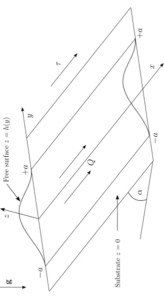
Consider the steady unidirectional flow of a thin rivulet on a planar substrate inclined at an angleαto the horizontal with constant semiwidthaand constant volume fluxQsubject to a prescribed uniform longitudinal surface shear stressτ. Cartesian axesOxyzare chosen with thex-axis down the slope, they-axis parallel to the substrate, and thez-axis normal to the substrate. The fluid is assumed to be Newtonian with constant densityρ, viscosity
µ, and surface tension γ. The velocity u = u(y, z)i and pressure p = p(x, y, z) of the fluid are governed by the familiar mass-conservation and Navier–Stokes equations subject to the usual normal and tangential stress balances and the kinematic condition at the free surface z = h(y), and no slip at the substrate z = 0. By definition the rivulet has zero thickness at its contact lines y = ±a, i.e. h(±a) = 0, and the contact angle θ is given by θ = ∓h0(±a), where the prime denotes differentiation with respect to argument. We
are primarily concerned with steady flow of a perfectly wetting fluid for which the contact angle is zero, i.e.θ= 0, as shown in Figure 1. However, the quasi-steady stability analysis described in Section 5 involves the unsteady evolution of a rivulet with non-zero contact angle, and with this in mind, it is appropriate to consider first the general caseθ6= 0 before considering the special caseθ= 0.
We consider a thin rivulet with a small transverse aspect ratio 1; in this case it is appropriate to non-dimensionalise y and a withl, z and hwith l, uwith U =ρg2l2/µ,
Q with l2U = ρg3l4/µ, p−p
∞ with ρgl and τ with ρgl, and scale θ with , where l= (γ/ρg)1/2is the capillary length,g is acceleration due to gravity andp
∞is the uniform
atmospheric pressure. Since the flow is unidirectional, the mass-conservation equation and kinematic boundary condition are identically satisfied, and at leading order inthe Navier– Stokes equation reduces to
0 = sinα+uzz, 0 =−py, 0 =−pz−cosα, (2.1)
to be solved subject to boundary conditions of no slip at the substrate,
u= 0 on z= 0, (2.2)
balances of normal and tangential stress at the free surface,
p=−h00 and u
PSfrag
replacemen
ts
x
y
z
g
τ
F
ree
surface
z
=
h
(
y
)
α
Substrate
z
=
0
+
a
+
a
−
a
−
a
Q
[image:4.612.110.438.72.663.2]∓ ±
Therefore we can readily obtain the solution
u=sinα
2 (2h−z)z+τ z, (2.5)
p= (h−z) cosα−h00. (2.6)
In particular, the free surface velocityus=us(y) =u(y, h) is given by
us=
sinα
2 h
2+τ h. (2.7)
Substituting (2.6) into the second equation in (2.1) yields a third-order ordinary differential equation for the free surface profileh, namely
(h00−cosα h)0 = 0, (2.8)
to be solved subject to (2.4). In the general caseθ6= 0 we obtain
h=θ×
coshma−coshmy
msinhma when 0≤α <
π
2,
a2−y2
2a when α=
π
2, cosmy−cosma
msinma when
π
2 < α≤π,
(2.9)
where m=p
|cosα|. In the special case θ= 0 Wilson and Duffy (26) showed that when 0≤α ≤π/2 there are no solutions for h, but that when π/2< α ≤π there is a simple solution corresponding to a pendent rivulet hanging underneath the substrate, namely
a= π
m (2.10)
and
h=hm
2 (1 + cosmy), (2.11)
where hm =h(0) is the (unknown) maximum height of the rivulet. As Wilson and Duffy
(26) showed, whenπ/2< α≤πthere are, in fact, infinitely many solutions, but since all the other solutions are simply appropriately re-scaled copies of (2.10) and (2.11) representing arrays of contiguous identical rivulets, we do not consider them any further here.
The local volume flux ¯u= ¯u(y) is given by
¯
u=
Z h
0
udz=sinα 3 h
3+τ
2h
and so the total volume flux down the rivuletQis given by
Q=
Z +a
−a
¯
udy= sinα 3
Z +a
−a
h3dy+τ
2
Z +a
−a
h2dy. (2.13)
In the general caseθ6= 0 we obtain
Q= θ
3sinα
9m4 f(ma) +
θ2τ
2m3g(ma), (2.14)
where the functions f = f(ma) and g = g(ma) (arising from the contributions due to gravity and surface shear stress effects, respectively) are given by
f(ma) =
15macoth3ma−15 coth2ma−9macothma+ 4 when 0≤α <π
2, 12
35(ma)
4 when α= π
2,
−15macot3ma+ 15 cot2ma−9macotma+ 4 when π
2 < α≤π, (2.15) and
g(ma) =
3macoth2ma−3 cothma−ma when 0≤α < π
2, 4
15(ma)
3 when α= π
2, 3macot2ma−3 cotma+ma when π
2 < α≤π.
(2.16)
The corresponding results of Wilson and Duffy (30,19) are recovered in the special case
τ = 0 and in the limitα→π/2+, respectively. In the special caseθ= 0 we obtain
Q= π
24m(5 sinα hm+ 9τ)h
2
m. (2.17)
If the flux takes the prescribed value Q = ¯Q, then (2.14) determines the appropriate value(s) ofawhenθ6= 0 and (2.17) determines the appropriate value(s) ofhm whenθ= 0.
Onceaorhm is known the rivulet solution given by (2.5), (2.6) and (2.9) (whenθ6= 0) or
(2.10) and (2.11) (whenθ= 0) is completely determined.
Henceforth (except for the quasi-steady stability analysis described in Section 5) we shall restrict our attention to the subject of this work, namely the steady flow of a rivulet of perfectly wetting fluid withθ= 0.
In the special case of no prescribed shear stress,τ = 0, the rivulet is purely gravity-driven and the equationQ= ¯Qhas the simple explicit solution obtained by Wilson and Duffy (26), namely
hm=
24 ¯Qm
5πsinα
1 3
. (2.18)
In the general caseτ 6= 0 the equationQ= ¯Qmay be written in the form
hmsinα
τ
3
+9 5
hmsinα
τ
2
=24 ¯Qmsin
2α
≥
solution corresponding to a rivulet with zero net flux, ¯Q= 0, given byhm=hm0, where
hm0=− 9τ
5 sinα. (2.20)
In the limit of large positive or negative shear stress,|τ| → ∞, the effect of shear stress dominates the effect of gravity and soτ and ¯Q must have the same sign, and at leading order inτ the rivulet is purely shear-driven andhmis given explicitly by
hm=
8 ¯Qm
3πτ
1 2
. (2.21)
In the limit of large positive flux, ¯Q→ ∞, the rivulet is deep (i.e.hm → ∞), and the
effect of gravity dominates the effect of shear stress, so that at leading orderhm is given
by (2.18). In the limit of small flux, ¯Q →0, either the rivulet becomes shallow, and the effect of shear stress dominates the effect of gravity, so that at leading orderhm is given by
(2.21), or, when τ <0, the effects of shear stress and gravity balance, so that the rivulet has finite height, given at leading order by (2.20).
3. Categorisation of Flow Patterns
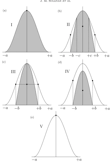
All of the possible cross-sectional flow patterns that can occur may be categorised into five types which, following the notation introduced by Wilson and Duffy (19) for a rivulet of non-perfectly wetting fluid on a vertical substrate, we denote as type I to type V. Figure 2 shows sketches of these five different types of flow pattern; regions of “downwards” flow (i.e. regions withu >0) are shaded, and regions of “upwards” flow (i.e. regions withu <0) are unshaded. The locations of the maximum and minimum velocities are marked with dots.
Whenτ ≥0 the prescribed shear stress acts down the substrate in cooperation with the effect of gravity. As a result, the velocity is downwards throughout the rivulet; we refer to this flow pattern as type I (see Figure 2(a)). The maximum velocityu=us(0) =u1(>0),
where
u1=hm
hmsinα
2 +τ
, (3.1)
occurs on the free surface aty= 0,z=hmand the minimum velocityu= 0 occurs on the
substratez= 0.
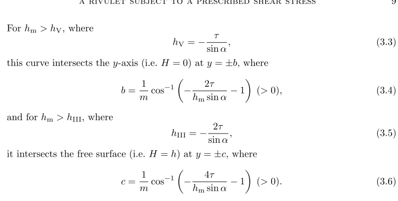
Whenτ <0, the prescribed shear stress acts up the substrate in opposition to the effect of gravity, and the competition between these opposing effects leads to more interesting behaviour than in the case τ ≥0. In particular, we find that, although the velocity can be downwards within the rivulet, it is always upwards near the edges of the rivulet. The non-trivial curve on whichu= 0, denoted by z=H(y), is given by
H = 2h+ τ
sinα
PSfrag replacements
(a) (b)
(c) (d)
(e)
−
a
−
a
−
a
−
a
−
a
+
a
+
a
+
a
+
a
+
a
−
b
−
b
−
b
+
b
+
b
+
b
−
c
+
c
III
IV
I
II
V
[image:8.612.108.486.64.616.2]this curve intersects they-axis (i.e.H = 0) aty=±b, where
b= 1
mcos −1
−h 2τ msinα−
1
(>0), (3.4)
and forhm> hIII, where
hIII=− 2τ
sinα, (3.5)
it intersects the free surface (i.e.H =h) aty=±c, where
c= 1
mcos −1
− 4τ
hmsinα−
1
(>0). (3.6)
When hm > hIII we have Hm = H(0) > hm, and we refer to this flow pattern as
type II (Figure 2(b)). When hm = hIII we have Hm = hm, b = a/2 and c = 0, and
the curve z = H just touches the free surface at y = 0, z = hm; we refer to this flow
pattern as type III (Figure 2(c)) and note that it is the marginal case between type II and type IV. When hV < hm < hIII we have 0 < Hm < hm and we refer to this flow
pattern as type IV (Figure 2(d)). For flow patterns II, III and IV the maximum velocity
u=u(0, Hm/2) =u1+u2(>0), where
u2=
τ2
2 sinα, (3.7)
occurs within the flow at y = 0, z =Hm/2 = hm+τ /sinα, and the minimum velocity
u=us(b) =−u2(<0) occurs on the free surface aty=±b,z=−τ /sinα.
Finally, whenhm≤hVthe prescribed shear stress dominates the effect of gravity and the
velocity is upwards throughout the rivulet; we refer to this flow pattern as type V (Figure 2(e)). The maximum velocity u = 0 occurs on the substrate z = 0, and the minimum velocityu=us(0) =u1(<0) occurs on the free surface aty= 0,z=hm.
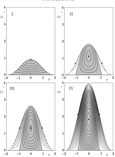
Four of the five flow patterns are illustrated in Figure 3, which shows the free surface profile and velocity contours in the caseα= 3π/4 and ¯Q= 1 forτ = 0.5 (type I),τ =−0.5 (type II),τ =τIII' −0.9295 (type III) andτ =−1.5 (type IV), where
τIII=−
6 ¯Qmsin2α
π
1 3
(<0) (3.8)
is the critical value ofτ corresponding tohm=hIII. The contour interval is constant and
the locations of the maximum and minimum velocities are marked with dots.
[image:9.612.89.492.66.270.2]4. Rivulet Solutions
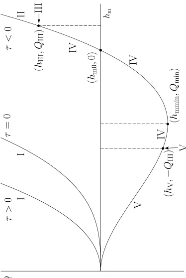
Figure 4 shows a sketch ofQgiven by (2.17) as a function ofhmforτ >0,τ = 0 andτ <0,
and summarises when the different types of flow pattern described in Section 3 occur. For
1
2
3
4
0
1
2
3
4
0
1
2
3
4
0
1
2
3
4
0
1
0
2
−1
−2
1
0
2
−2
1
0
2
−1
−2
1
0
2
−2
−1
−1
PSfrag replacements
z
z z
z
y
y y
y
(a) (b)
(c) (d)
I
II
III
IV
Fig. 3 Free surface profile and velocity contours in the caseα= 3π/4 and ¯Q= 1 for (a)τ = 0.5 (type I), (b) τ = −0.5 (type II), (c) τ = τIII ' −0.9295 (type III), and (d) τ = −1.5 (type
[image:10.612.105.487.68.590.2]PSfrag
replacemen
ts
Q
τ
>
0
τ
=
0
τ
<
0
(
h
V
,
−
Q
II
I
)
(
h
mmin
,Q
min
)
(
h
m0
,
0)
(
h
II
I
,Q
II
I
)
I
I
IV
IV
IV
V
V
Fig. 4 Sketch ofQas a function ofhmforτ >0,τ= 0 andτ <0, summarising when the different
[image:11.612.95.469.80.638.2]contrast, forτ <0,Qinitially decreases monotonically to a minimum value Q=Qmin at
hm=hmmin, where
Qmin=− 9π(−τ) 3
50msin2α (<0), hmmin=−
6τ
5 sinα, (4.1)
before increasing monotonically through the valueQ= 0 athm=hm0given by (2.20), and
tending to infinity ashm→ ∞.
As Figure 4 shows, the number and nature of solutions forhmdepends on the values ofτ,
αand ¯Q. Whenτ ≥0, there is one solution (of type I) when ¯Q >0, but no solutions when ¯
Q≤ 0. When τ <0, there is one solution when ¯Q≥ 0 (which is of type II and satisfies
hm > hIII for ¯Q > QIII, of type III given by hm =hIII for ¯Q=QIII, and of type IV and
satisfieshm0≤hm< hIIIfor 0≤Q < Q¯ III, where
QIII= π(−τ) 3
6msin2α(>0) (4.2)
is the critical value of ¯Qcorresponding tohm=hIII). When ¯Q <0 there are two solutions
whenQmin<Q <¯ 0, a “thick” solution (which is of type IV satisfyinghmmin< hm< hm0)
and a “thin” solution (which is of type V satisfying 0< hm ≤hV for−QIII≤Q <¯ 0 and
of type IV satisfyinghV < hm < hmmin for Qmin<Q <¯ −QIII), one solution (of type IV
given byhm=hmmin) when ¯Q=Qmin, and no solutions when ¯Q < Qmin.
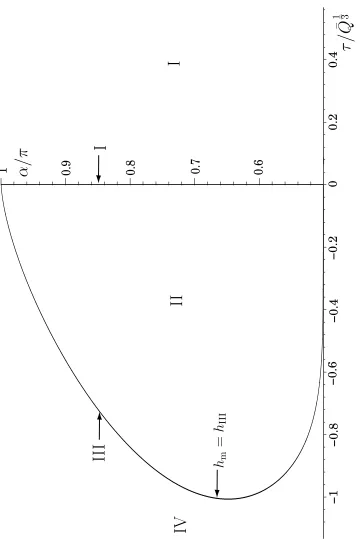
Figure 5 shows how the τ /Q¯13–α parameter plane for ¯Q > 0 is divided into regions in
which the solutions have different flow patterns by the αaxis and the curvehm=hIII for
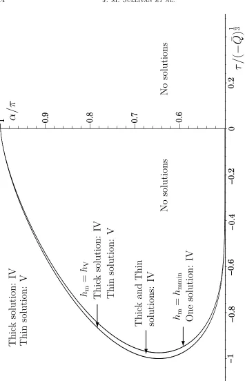
τ <0, and Figure 6 shows how theτ /(−Q¯)13–αparameter plane for ¯Q <0 is divided into
regions in which the solutions have different flow patterns by the curvehm=hVforτ <0,
and into regions in which there are no or two solutions by the curvehm=hmminforτ <0
on which there is one solution.
4.1 Rivulet Solutions for Varying α
As well as being of interest in their own right, rivulet solutions for varying α can be interpreted as describing flow down a slowly varying substrate such as, for example, flow in the azimuthal direction round the lower part of a large horizontal cylinder.
Whatever the values ofτ and ¯Q, the rivulet semiwidth is given by a=π/mand so all rivulets become wide according to
a∼πα−π2−
1 2
→ ∞ (4.3)
asα→π/2+, and approach the finite semiwidtha=π according to
a=π+π
4(π−α)
2
+O(π−α)4 (4.4)
asα→π−.
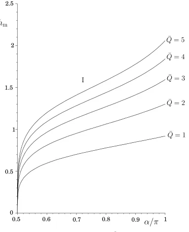
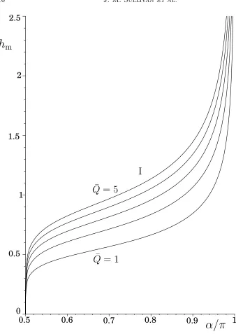
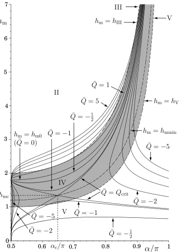
Figures 7, 8 and 9 show hm as a function of αin the casesτ = 1, τ = 0 and τ =−1,
respectively, for various values of ¯Q; these are typical of hm for all τ >0,τ = 0 andτ <0,
0.6
0.7
0.
8
0.
9
1
0
0.
2
0.
4
−1
−0.2
−0.4
−0.6
−0.8
PSfrag
replacemen
ts
α
/π
α
c
/π
'
0
.
6476
τ
/
h
m=
h
III
I
I
II
II
I
IV
V
Fig. 5 Plot of theτ /Q¯13–αparameter plane for ¯Q >0 divided into regions in which the solutions
[image:13.612.99.461.79.621.2]0.
2
0
−1
0.
6
0.
7
0.8
0.9
1
−0.2
−0.4
−0.6
−0.8
PSfrag
replacemen
ts
α
/π
α
c
/π
'
0
.
6476
τ
/
(
−
¯
Q
)
1 3h
m=
h
mminh
m=
h
VThic
k
solution:
IV
Thic
k
solution:
IV
Thin
solution:
V
Thin
solution:
V
Thic
k
and
Thin
solutions:
IV
One
solution:
IV
No
solutions
No
solutions
I II
II
I
IV V
Fig. 6 Plot of the τ /(−Q)¯ 13–α parameter plane for ¯Q < 0 divided into regions in which the
solutions have different flow patterns by the curvehm =hV for τ <0, and into regions in which
[image:14.612.99.454.67.619.2]1
0.5
1.5
2
0
0.5
0.6
0.7
0.8
0.9
1
PSfrag replacements
h
m
α/π
¯
Q
= 1
¯
Q
= 2
¯
Q
= 3
¯
Q
= 4
¯
Q
= 5
I
[image:15.612.101.484.85.556.2]0.5
0.6
0.7
0.8
0.9
1
1
0.5
1.5
2
2.5
0
PSfrag replacements
α/π
h
m
¯
Q
= 5
¯
Q
= 1
I
Fig. 8 Plot ofhm as a function ofαin the special caseτ = 0 for ¯Q= 1, . . . ,5. All solutions are
[image:16.612.99.437.67.544.2]0.5
0.6
0.7
0.8
0.9
1
0
4
5
6
1
3
2
PSfrag replacements
α/π
h
m
h
m=
h
Vh
m=
h
mminh
m=
h
IIIh
m=
h
m0h
mcα
c/π
( ¯
Q
= 0)
¯
Q
=
−
1
¯
Q
=
Q
crit¯
Q
=
−
5
¯
Q
= 5
¯
Q
= 1
¯
Q
=
−
5
¯
Q
=
−
2
¯
Q
=
−
1
¯
Q
=
−
2
¯
Q
=
−
12¯
Q
=
−
12I
II
IV
V
V
Fig. 9 Plot ofhmas a function ofαin the caseτ =−1 for ¯Q=−5, . . . ,5. Also shown are regions
in which the solutions have different flow patterns divided by the curveshm=hIIIandhm=hV
(shown with dashed curves), and the curve hm =hmmin (also shown with a dashed curve). For
[image:17.612.102.469.82.598.2]4.1.1 τ >0
Figure 7 showshm as a function ofαin the caseτ = 1 for ¯Q= 1, . . . ,5. There is a single
solution for hm everywhere (i.e. for all π/2 < α ≤ π) for each value of ¯Q (> 0) and all
solutions are of type I. In this case (i.e. whenτ >0) the rivulets become shallow according to
hm∼
8 ¯Q
3πτ
1 2
α−π
2
14
→0+ (4.5)
asα→π/2+, and approach the finite heighth
m=hmπ= (8 ¯Q/3πτ)
1
2 according to
hm=hmπ− 20 ¯Q
27πτ2(π−α) +O(π−α)
2 (4.6)
asα→π−.
4.1.2 τ = 0
Figure 8 showshmgiven by (2.18) as a function ofαin the special caseτ = 0 for ¯Q= 1, . . . ,5.
There is again a single solution forhm everywhere (i.e. for allπ/2< α≤π) for each value
of ¯Q(>0) and all solutions are of type I. In this case (i.e. whenτ = 0) the rivulets become shallow according to
hm∼
24 ¯Q
5π
1 3
α−π
2
16
→0+ (4.7)
as α→π/2+, and become deep (and hence the assumption that the rivulet is sufficiently
slowly varying inαultimately fails) according to
hm∼
24 ¯Q
5π
1 3
(π−α)−13 → ∞ (4.8)
asα→π−.
4.1.3 τ <0
Figure 9 showshmas a function ofαin the caseτ =−1 for ¯Q=−5, . . . ,5, and, as expected,
reveals that the behaviour whenτ <0 is more complicated than whenτ ≥0. Specifically, for each value of ¯Q≥0, there is a single solution forhmeverywhere (i.e. for allπ/2< α≤π)
satisfyinghm≥hm0. However, when ¯Q <0 there can be one, two or no solutions forhm
(all satisfyinghm< hm0) depending on the values ofτ,αand ¯Q. ForQcrit<Q <¯ 0, where
Qcrit=−
9×514π(−τ)3
40 ' −1.0570(−τ)
3(<0), (4.9)
there are two disconnected branches of solutions forhm, each of which extends all the way
fromα=π/2+ toα=π, that is, there is both a thick and a thin solution everywhere. As
¯
Qdecreases from zero towardsQcrit these two branches of solutions move closer together,
1 2 m mmin 1 m mmin 2
respectively, whereα1andα2(> α1) are the appropriate solutions of ¯Q=Qmin; thus there
are no solutions forα1< α < α2, one solution atα=α1 andα=α2, and two solutions for
π/2< α < α1andα2< α≤π. Thus, unlike the caseτ ≥0 in which a slowly varying rivulet
can run continuously round the lower part of a large horizontal cylinder fromα=π/2+to
α=π forany Q¯(>0), whenτ <0 this can happen only when ¯Q≥Qcrit.
In this case (i.e. whenτ <0) both the single solution for ¯Q≥0 and the thick solution for ¯Q <0 approach the finite heighthm=hmπ
2 =−9τ /5 according to
hm=hmπ
2 +
40 ¯Q
27πτ2
α−π
2
12
+Oα−π
2
(4.10)
as α → π/2+, while the thin solution for ¯Q < 0 becomes shallow according to (4.5) as
α→π/2+. Similarly, both the single solution for ¯Q≥0 and the thick solution for ¯Q <0
become deep according to
hm∼ −
9τ
5 (π−α) → ∞ (4.11)
as α → π−, while the thin solution for ¯Q < 0 approaches the finite height h
m = hmπ =
(8 ¯Q/3πτ)12 according to (4.6) asα→π−.
In the special case ¯Q=Qcrit the fact that the two branches of solutions meet atα=αc
means that four different kinds of behaviour are possible for varyingα: a rivulet could be thin everywhere, thick everywhere, thin inπ/2< α < αc and thick inαc < α≤π, or thick
inπ/2< α < αc and thin inαc< α≤π. In the first two cases the rivulet has a corner at
α=αc†, whereas in the latter two cases the rivulet is smooth atα=αc.
Figure 9 also shows how theα–hm parameter plane is divided into regions in which the
solutions have different flow patterns by the critical curveshm=hIIIandhm=hV(shown
with dashed curves). In particular, when ¯Q > QIIIc, where
QIIIc=5
5
4π(−τ)3
24 '0.9787(−τ)
3(>0) (4.12)
is the value ofQIII given by (4.2) atα=αc, solutions are of type II forαIII1< α < αIII2,
type III atα=αIII1andα=αIII2, and type IV elsewhere, whereαIII1 andαIII2(> αIII1)
are the appropriate solutions of ¯Q=QIII and satisfyαIII1< αc < αIII2. When ¯Q=QIIIc
solutions are of type IV everywhere except atα=αc (where they are of type III), and when
0≤Q < Q¯ IIIcthey are of type IV everywhere. When ¯Q <0 all thick solutions are of type
IV everywhere, while thin solutions for−QIIIc≤Q <¯ 0 are of type V everywhere and thin
solutions for ¯Q <−QIIIc are of type IV forαIII1< α < αIII2and of type V elsewhere.
Thus the flow pattern within a slowly varying rivulet may change as it flows round the lower part of a large horizontal cylinder. For a rivulet with ¯Q > QIIIc the flow pattern
changes from type IV for π/2< α < αIII1 to type III at α=αIII1, to type II for αIII1 <
†This corner in the critical rivulet is analogous to the well known corner in the critical solution in coating
PSfrag replacements
IV
IV
V
II
III
III
Free surface
Cylinder
g
−
τ
(
>
0)
α
=
α
III1
[image:20.612.104.492.82.500.2]α
=
α
III2
Fig. 10 Sketch of the streamline pattern in the symmetry plane,y= 0, of a slowly varying rivulet on the lower part of a large horizontal cylinder when τ < 0 in the case ¯Q > QIIIc. Regions of
downwards flow (i.e. regions withu >0) are shaded and regions of upwards flow (i.e. regions with u <0) are unshaded.
α < αIII2, to type III at α = αIII2, to type IV for αIII2 < α ≤ π. On the other hand,
for a thin rivulet with Qcrit ≤ Q <¯ −QIIIc the flow pattern changes from type V for
π/2< α≤αIII1 to type IV forαIII1< α < αIII2, to type V forαIII2≤α≤π, whereαIII1
and αIII2 satisfyαIIImin≤αIII1 < αc and αc < αIII2 ≤αIIImax, where αIIImin '0.5950π
PSfrag replacements
IV
V
V
V
V
II
III
Free surface
Cylinder
g
−
τ
(
>
0)
α
=
α
III1
[image:21.612.100.506.85.424.2]α
=
α
III2
Fig. 11 Sketch of the streamline pattern in the symmetry plane,y= 0, of a slowly varying rivulet on the lower part of a large horizontal cylinder whenτ <0 in the caseQcrit<Q <¯ −QIIIc. Regions
of downwards flow (i.e. regions withu >0) are shaded and regions of upwards flow (i.e. regions withu <0) are unshaded.
and ¯Q=Qcrit. The streamline patterns in the symmetry plane of the rivulet, y = 0, are
sketched Figures 10 and 11, respectively, in these two cases. In particular, Figure 10 shows the regions of backflow that will occur inπ/2< α < αIII1andαIII2< α≤π for ¯Q > QIIIc,
and Figure 11 shows the recirculation “bubble” of “trapped” fluid in αIII1 < α < αIII2
that will occur for Qcrit ≤ Q <¯ −QIIIc, as consequences of the competition between the
(downwards) effect of gravity and the (upwards) effect of the prescribed shear stress. The “footprints” on the substrate of the regions of backflow in Figure 10 and of the recirculation region in Figure 11 are given by|y| ≤b, whereb(≤a) is defined by (2.17) and (3.4) with
2
4
−2
−4
2
3
4
1
0
5
PSfrag
replacemen
ts
h
m
τ
¯
Q
=
1
¯
Q
=
5
¯
Q
=
−
5
¯
Q
=
−
1
h
m
=
h
m0
(
¯
Q
=
0)
h
m
=
h
mmin
h
m
=
h
V
h
m
=
h
II
I
I
I
II
II
I
IV
V
[image:22.612.98.483.85.595.2]V
Fig. 12 Plot ofhm as a function of τ in the caseα= 3π/4 for ¯Q=−5, . . . ,5. Also shown are
regions in which the solutions have different flow patterns divided by the curveshm = hIII and
hm=hV(shown with dashed curves), and the curvehm=hmmin(also shown with a dashed curve).
external airflow exerting a uniform shear stress whose strength varies slowly in time. Figure 12 showshm as a function ofτ in the case α= 3π/4 for ¯Q=−5, . . . ,5 which is
typical ofhmfor allπ/2< α≤π.
As Figure 12 shows, for ¯Q≥0 there is a single solution for hmfor all τ. In the limit of
large positive shear stress,τ → ∞, the rivulet becomes shallow according to
hm∼
8 ¯Qm
3πτ
1 2
→0+, (4.13)
while in the limit of large negative shear stress,τ → −∞, the rivulet becomes deep according to
hm∼hm0=− 9τ
5 sinα → ∞. (4.14)
In the limit of small shear stress,τ →0, the rivulet approaches the finite height in the case
τ = 0 given by (2.18) according to
hm=
24 ¯Qm
5πsinα
1 3
− 3τ
5 sinα+O(τ
2). (4.15)
As Figure 12 also shows, for ¯Q < 0 there are no solutions for hm when τmin < τ ≤ 0,
one solutionhm=hmmin whenτ =τmin, and two solutions (one thin and one thick) when
τ < τmin, where
τmin=
50 ¯Qmsin2α
9π
1 3
(<0) (4.16)
is the critical value of τ corresponding to ¯Q=Qmin. In the limit of large negative shear
stress,τ → −∞, the thin rivulet becomes shallow according to (4.13) and the thick rivulet becomes deep according to (4.14).
Figure 12 also shows how theτ–hmparameter plane is divided into regions in which the
solutions have different flow patterns by the critical curveshm=hIIIandhm=hV(shown
with dashed curves).
5. Quasi-Steady Stability
Having determined and classified all of the possible rivulet solutions, the next step is to consider whether or not these rivulets are stable.
A full stability analysis is beyond the scope of the present work, but we can make useful progress by considering the quasi-steady stability of a rivulet to small symmetric perturbations, i.e. the stability to symmetric perturbations in the limit in which the contact line moves slowly relative to the bulk of the fluid.
A perturbation to a steady rivulet with zero contact angle will, in general, lead to an unsteady rivulet with a non-zero contact angle. Thus we consider the quasi-steady stability of a pendent rivulet with static contact angle θ0 (>0) and semi-widtha0 on a substrate
Following the approach of the earlier work on the quasi-steady stability of a rivulet of non-perfectly wetting fluid by Wilson and Duffy (30,19), we assume that the flow remains symmetric and unidirectional, and that the quasi-steady motion is driven by that of the moving contact liney=a, wherea=a(t). We assume that the speed of the moving contact line,a0, and the dynamic contact angle,θ=θ(t), are related by an empirically determined
“Tanner Law” in the rather general forma0=F(θ), where the functionF =F(θ) satisfies F(θ0) = 0 and is monotonically increasing near θ =θ0. We perturb the basic state with
semi-widtha=a0and contact angleθ=θ0by writinga(t) =a0+a1(t) andθ(t) =θ0+θ1(t),
where|a1| a0 and|θ1| θ0 are small perturbations, so that
a0 1=
M θr
1
r! , (5.1)
whereM= drF/dθr|
θ=θ0 (>0) is the first non-zero (odd) derivative ofF(θ) evaluated at
θ=θ0. The perturbed rivulet must satisfy the prescribed flux conditionQ= ¯Q, whereQis
given by the general expression for a rivulet with non-zero contact angle derived in Section 2, namely (2.14), and hence
a1∂Q
∂a +θ1 ∂Q
∂θ = 0 (5.2)
evaluated ata=a0andθ=θ0, meaning that
θ1=σa1, (5.3)
whereσ is given by
σ =−∂Q/∂a
∂Q/∂θ
a=a
0,θ=θ0
=−mθ0[2θ0sinαf
0(ma
0) + 9mτ g0(ma0)]
6 [θ0sinαf(ma0) + 3mτ g(ma0)]
, (5.4)
in which the functions f(ma) and g(ma) are given by (2.15) and (2.16), respectively. Combining (5.1) and (5.3) the equation satisfied bya1 is
a0 1=
M(σa1)r
r! , (5.5)
so thata1 is given by
a1=a1(0)
eσM t if r= 1,
1− (r−1)M σ
r
r!(a1(0))1−r
t
1 1−r
if r= 3,5,7, . . . , (5.6)
where a1(0) is the value of a1 at t = 0. Hence small perturbations grow or decay
exponentially when r = 1 and algebraically whenr = 3,5,7, . . ., and (since bothM and
rare positive), the stability of the rivulet depends only on the sign of σ. In the perfectly wetting limit,θ0→0, the semi-width of the basic statea=a0 approaches the valueπ/m
in (2.10) according to
a0= π
m+
θ0
σ +O(θ
2
Q=− 3m7 σ +2m5σ . (5.8)
Then the equationQ= ¯Qwith Qgiven by (5.8) yields a cubic polynomial equation forσ, namely
10πsinα σ3−9πτ m2σ2+ 6 ¯Qm7= 0. (5.9) For the rivulet not to be unstable we require all the real roots of (5.9) to be negative (for stability) or zero (for neutral stability). When ¯Q >0 equation (5.9) has three real roots whenτ ≥τs (two of them positive and one negative), and has one (negative) real root and
two complex roots whenτ < τs, where
τs=
50 ¯Qmsin2α
9π
1 3
(>0); (5.10)
hence, in this case the rivulet is stable when τ < τs and unstable when τ ≥ τs. When
¯
Q= 0 (and hence necessarilyτ <0) equation (5.9) always has three real roots (one of them negative and the other two zero); hence, in this case the rivulet is always neutrally stable. When ¯Q <0 (and hence necessarilyτ <0) equation (5.9) always has one positive real root; hence, in this case the rivulet is always unstable.
Figure 13 shows how the τ–hm parameter plane is divided into stable (shaded) and
unstable (unshaded) regions according to the present quasi-steady stability analysis. Specifically, Figure 13 shows that for τ > 0 rivulets with hm ≤ hms are unstable and
rivulets withhm> hms are stable, where
hms= 3τ
5 sinα (5.11)
is the critical value of hm corresponding to τ = τs. Figure 13 also shows that forτ ≤ 0
rivulets withhm> hm0,hm=hm0andhm< hm0are stable, neutrally stable and unstable,
respectively, wherehm0 is given by (2.20). Figure 13 also includes the solutions forhm for
¯
Q = −5, . . . ,5 (i.e. exactly the same solutions as those shown in Figure 12) in order to indicate which are stable and which are unstable.
6. Rivulet Splitting
Having investigated the quasi-steady stability of the present rivulet solutions to small perturbations in Section 5, in this section we determine the conditions under which it is energetically favourable for them to split into subrivulets. In particular, we extend and generalise the recent work of Wilson and Duffy (19,27) to determine when it is energetically favourable for a rivulet of perfectly wetting fluid on an inclined substrate subject to a prescribed longitudinal surface shear stress to split into one or more subrivulets.
0
2
4
−2
−4
1
2
3
4
PSfrag
replacemen
ts
h
m
τ
h
m
=
h
m0
(
¯
Q
=
0)
h
m
=
h
ms
¯
Q
=
−
5
¯
Q
=
5
¯
Q
=
−
1
¯
Q
=
1
Unstable
Unstable
[image:26.612.102.512.77.604.2]Stable
Fig. 13 Plot of theτ–hmparameter plane divided into stable (shaded) and unstable (unshaded)
1
2 −a 0
u2(y, z) dzdy, (6.1)
and the surface energy per unit length of a rivulet, or, more precisely, the difference between the surface energy of a rivulet and the surface energy of the same width of dry substrate per unit length, is given by
1
2W
Z +a
−a
1 +2h02
1 2
dy−2a
, (6.2)
where
W = ρlU
2
γ =
γ23
glµ2 (6.3)
is an appropriately defined Weber number. Thus, the leading-order expression for the total energy per unit length of a rivulet,E, is given by
E= 1
120
Z +a
−a
8h2sin2α+ 25τ hsinα+ 20τ2
h3dy+ 1 2W
Z +a
−a
h02dy, (6.4)
which can be evaluated to give
E= π
7680m 252h
2
msin2α+ 875τ hmsinα+ 800τ2h3m+
mπ
8Wh
2
m. (6.5)
In the special case τ = 0 equation (6.5) reduces to the corresponding expression obtained by Wilson and Duffy (27) for a purely gravity-driven rivulet of perfectly wetting fluid.
Before proceeding any further it is convenient to scale αand W out of the problem by writing
τ =
m2sinα
W
13
ˆ
τ , hm=
m2
Wsin2α
13
ˆ
hm,
E=
m7
W5sin4α
1 3
ˆ
E, Q= m
WsinαQ,ˆ
(6.6)
and to drop the hats in the remainder of this section for clarity to give simplified expressions for the flux (2.17), namely
Q= π
24(5hm+ 9τ)h
2
m (6.7)
and the total energy (6.5), namely
E= π
7680 252h
3
m+ 875τ h2m+ 800τ2hm+ 960h2m. (6.8)
We shall consider two specific problems concerning the splitting of a rivulet, namely splitting into two, in general, non-identical subrivulets, and splitting inton(n= 1,2,3, . . .) identical subrivulets.
It is energetically favourable for a rivulet with maximum heighthmand flux ¯Qto split into
height hm(1−λ) and flux (1−λ) ¯Q, where, by conservation of mass, hmλ and hm(1−λ) are
related by
(5hm+ 9τ)hm2 = (5hmλ+ 9τ)hm2λ+ (5hm(1−λ)+ 9τ)h2m(1−λ), (6.9)
when the difference between the energies of the two states, ∆E, defined by ∆E=E−
E(hm=hmλ) +E(hm=hm(1−λ)), (6.10)
is positive. If there is a range of energetically favourable values of λ then the most energetically favourable state is the one with the lowest energy and hence thelargestpositive value of ∆E.
Similarly, it is energetically favourable for a rivulet of maximum heighthm and flux ¯Q
to split inton(n= 1,2,3, . . .) identical subrivulets each of maximum heighthmn and flux
¯
Q/n, where, by conservation of mass,hmand hmn are related by
(5hm+ 9τ)h2m=n(5hmn+ 9τ)h2mn, (6.11)
when the difference between the energies of the two states, ∆En, defined by
∆En =E−nE(hm=hmn), (6.12)
is positive. If there is more than one energetically favourable state then the most energetically favourable state is the one with the lowest energy and hence thelargestpositive value of ∆En. A state withnsubrivulets has the same energy as a state withn+1 subrivulets
when the difference between the energies of the two states, ∆En,n+1, defined by
∆En,n+1= ∆En+1−∆En, (6.13)
is zero.
6.1 Purely Gravity-Driven Rivulet
Wilson and Duffy (27) examined the case of a purely gravity-driven rivulet (i.e. the case
τ = 0) for which, from (2.18),hm= (24 ¯Q/5π)
1
3, so that from (6.10) the energy difference
∆E is given by
∆E= 21π 640
24 ¯Q
5π
5
3
1−λ53 −(1−λ) 5
3 + 50π
63 ¯Q
n
1−λ23 −(1−λ) 2 3
o
, (6.14)
where λmust lie in the interval 0 ≤λ≤1. In this case ∆E <0 for all 0< λ <1 when
hm < hmc(2), ∆E = 0 at λ = 1/2 when hm = hmc(2), and ∆E has a positive global
maximum atλ= 1/2 when hm> hmc(2), where
hmc(2) =
"
80(231−1)
21(1−2−2
3)
#13
'1.3883. (6.15)
Hence it is energetically favourable for a rivulet to split into two subrivulets when hm >
hmc(2), and when this condition holds it is always most energetically favourable for the
n
∆En=
21π
640
24 ¯Q
5π
5
3
1−n−2
3 + 50π
63 ¯Q
n
1−n13
o
(6.16)
so that ∆En= 0 whenhm=hmc(n), where
hmc(n) =
"
80(n31−1)
21(1−n−2
3)
#
1 3
. (6.17)
Hence it is energetically favourable for a rivulet to split into n (n = 2,3,4, . . .) identical subrivulets when hm > hmc(n). The condition ∆En,n+1 = 0, where ∆En,n+1 is given
by (6.13), yields the critical value ofhm at which the most energetically favourable state
switches from one with n subrivulets to one with n+ 1 subrivulets. Hence the most energetically favourable state is the original rivulet (i.e. n = 1) for 0 < hm < hmc1, the
two-subrivulet (i.e. n = 2) state for hmc1 < hm < hmc2, the three-subrivulet (i.e. n = 3)
state forhmc2< hm< hmc3, and so on, where
hmcn=
80n(n+ 1)13 −n 1 3
o
21nn−2
3 −(n+ 1)−
2 3 o 1 3 . (6.18)
This critical value ofhmis equivalent to the corresponding critical value ofW obtained by
Wilson and Duffy (27, equation 12). Note thathmc1=hmc(2).
6.2 Purely Shear-Driven Rivulet
Also of interest is the case of a purely shear-driven rivulet (i.e. the leading order solution in the limit |τ| → ∞) for which, from (2.21), hm = (8 ¯Q/3πτ)1/2, so that from (6.10) the
energy difference ∆E is given by
∆E=
50τQ¯3
243π
1 2
h
1−λ32 −(1−λ) 3 2
i
, (6.19)
where λmust again lie in the interval 0≤λ≤1. In this case, whatever the value of hm,
∆E >0 for all 0< λ <1 and ∆Ealways has a positive global maximum atλ= 1/2, and so it isalwaysenergetically favourable for a rivulet to split into two subrivulets and, moreover, it is always most energetically favourable for the rivulet to split into identical subrivulets each with half the flux of the original. Similarly, from (6.12) the corresponding expression for the energy difference ∆En is
∆En=
50τQ¯3
243π
1 2
(1−n−1
2), (6.20)
and, since ∆En >0 forn >1, it isalwaysenergetically favourable for a rivulet to split into
n(n= 2,3,4, . . .) identical subrivulets. Moreover, since ∆En is a monotonically increasing
6.3 General Case
As the results in Subsections 6.1 and 6.2 show, in the special cases of a purely gravity-driven and a purely shear-gravity-driven rivulet, when it is energetically favourable for a rivulet to split into two subrivulets, it is always most energetically favourable for the subrivulets to be identical. Thus for simplicity in the general case in which both gravity and shear stress effects are significant treated in this subsection, we shall consider only splitting into
[image:30.612.96.492.451.653.2]n(n= 1,2,3, . . .) identical subrivulets
Figure 14 summarises all of the key results on rivulet splitting obtained in the present work in theτ–hmparameter plane. In particular, Figure 14 shows the (shaded) region of the
parameter plane bounded byhm=hm0=−9τ /5 forτ <0 and the curve ∆E2= 0 in which
it is unfavourable for a rivulet to split, and that whenτ ≥τc, whereτc = (2/3)
1
3 '0.8736,
and when hm < hm0 (including the curve hm = hmmin = −6τ /5) for τ < 0 the most
energetically favourable state is that with infinitely many subrivulets. The remainder of the parameter plane is divided by the critical curves ∆En = 0 forn= 3,4,5, . . . (shown with
dashed curves) into regions in which the state withnsubrivulets is energetically favourable, and by the critical curves ∆En,n+1 = 0 for n= 2,3,4, . . . (shown with solid curves) into
regions in which the state withnsubrivulets is the most energetically favourable. It is convenient to consider the cases ¯Q≥0 and ¯Q <0 separately in what follows.
6.3.1 Non-Negative Flux Q¯≥0
Examining the energy difference ∆En reveals that ∂∆En/∂n > 0 for all hm for n =
2,3,4, . . . when τ > τc but not when τ < τc. Hence we deduce that when τ > τc it is
always energetically favourable for a rivulet to split inton(n= 2,3,4, . . .) subrivulets and, moreover, that the most energetically favourable state is always that with infinitely many subrivulets.
As Figure 14 shows, the behaviour of a rivulet when ¯Q > 0 for 0< τ < τc and when
¯
Q≥0 forτ ≤0 (i.e.hm≥hm0 forτ ≤0) is rather more complicated.
To make analytical progress it is convenient to writehmn in terms of hm by introducing
a new parameterk(>0) according to
hmn=khm, (6.21)
and hence, from (6.11),hmis given in terms ofk by
hm=−9τ(1−nk 2)
5(1−nk3) (6.22)
which, from (6.12), gives ∆En in terms ofnandkas
∆En= 81πτ
2(1−nk2)3
16×105(1−nk3)5
8000(1−nk3)3−τ3Fn3
, (6.23)
where we have defined
Fn3= 12000(1−nk3)3
+189 5 (1−nk
2)
324(1−nk2)(1−nk5)−625(1−nk3)(1−nk4)
3
2
1
−2
−1
1
0
4
PSfrag
replacemen
ts
h
m
h
m=
h
m0h
m=
h
mminτ
c=
2
3
1 3
n
→
∞
τ
=
τ
c=
Infinitely
Infinitely
man
y
subrivulets
man
y
subrivulets
Unfa
vourable
to
split
n
=
2
3
4
5
6
10
50
100
[image:31.612.97.464.73.555.2]1000
Fig. 14 Plot of theτ–hmparameter plane showing the (shaded) region bounded byhm=hm0=
−9τ /5 forτ <0 and the curve ∆E2= 0 in which it is unfavourable for a rivulet to split, and that
whenτ ≥τc= (2/3)
1
3 '0.8736 and whenhm< hm0 (including the curvehm =hmmin=−6τ /5)
for τ < 0 the most energetically favourable state is that with infinitely many subrivulets. The remainder of the parameter plane is divided by the critical curves ∆En = 0 for n = 3,4,5, . . .
(shown with dotted curves) into regions in which the state with n subrivulets is energetically favourable, and by the critical curves ∆En,n+1 = 0 forn= 2,3,4, . . . (shown with solid curves)
From (6.22) and (6.23) the critical curves ∆En = 0 have the parametric representation
τ = 20
Fn(1−nk
3), h
m=−36
Fn(1−nk
2) (6.25)
with parameter k. The critical curves ∆En = 0 pass through the point hm = 0, τ = τc
(which corresponds to k=n−1
2), and intersectτ = 0 (which corresponds to k=n− 1
3) at
hm =hmc(n) given by (6.17). In the limit τ →τc− the critical curves ∆En = 0 approach
hm= 0 linearly inτc−τ according to
hm∼ 96n
1
2(τ
c−τ)
35(n12 + 1) →
0+. (6.26)
In the limit τ → −∞(which corresponds to k→kmax(n)−, where kmax =kmax(n) is the
unique real positive root ofFn = 0 fork) the critical curves ∆En = 0 become linear inτ
according to
hm∼ −
9τ(1−nk2 max)
5(1−nk3 max)
→ ∞, (6.27)
and so kmax(2) ' 0.9200 and hm ∼ −2.2373τ, kmax(3) ' 0.8758 and hm ∼ −2.3068τ,
kmax(4)'0.8454 andhm∼ −2.3616τ, andkmax(n) =O(n−
1
5)→0+andh
m=−O(n
1
5)τ →
∞asn→ ∞. The behaviour of the critical curves ∆En = 0 in the limitn→ ∞depends on
the sign onτ. When τ >0 the critical curves ∆En = 0 approach the finite limiting curve
hm=−
5h175τ2−p
7τ(3072−233τ3)i
504τ (6.28)
from below asn→ ∞. On the other hand, whenτ ≤0 the critical curves ∆En= 0 become
large likeO(n19) according to
hm∼
80 21
13
n19 '1.5618n 1
9 → ∞ (6.29)
whenτ = 0 and likeO(n15) according to
hm∼ −9τ
5
(3111τ3−40000)n
61236τ3
1 5
→ ∞ (6.30)
whenτ <0 asn→ ∞. Details of the relevant calculations are given in Appendix B. Similarly, it is convenient to writehm in terms ofhmn andhm(n+1) by defining the new
parameterskn(>0) andkn+1(>0) according to
hmn=knhm, hm(n+1)=kn+1hm (6.31)
and hence, from (6.11),hmis given in terms ofkn andkn+1by
hm=−
9τ(1−nk2
n)
5(1−nk3
n)
=−9τ
1−(n+ 1)kn2+1
5
1−(n+ 1)k3
n+1
=−9τ
(n+ 1)kn2+1−nk2n
5
(n+ 1)k3
n+1−nk3n
∆En,n+1=
16×105
nk3
n−(n+ 1)kn3+1
5 8000 nkn−(n+ 1)kn+1 −τ Fn,n+1 ,
(6.33) where we have defined
Fn,n3 +1= 12000
nk3n−(n+ 1)kn3+1 3
+189 5
nk2n−(n+ 1)kn2+1
324
nk2n−(n+ 1)k2n+1
nk5n−(n+ 1)kn5+1 −625
nk3n−(n+ 1)kn3+1
nkn4−(n+ 1)k4n+1
. (6.34)
From (6.32) and (6.33) the critical curves ∆En,n+1= 0 have the parametric representation
τ = 20
Fn,n+1
nk3n−(n+ 1)kn3+1 , hm=−
36
Fn,n+1
nk2n−(n+ 1)kn2+1 (6.35)
with parameters kn and kn+1. The critical curves ∆En,n+1 = 0 pass through the point
hm = 0, τ =τc (which corresponds tokn =n−
1
2, k
n+1 = (n+ 1)−
1
2) and intersect τ = 0
(which corresponds tokn=n−
1
3,k
n+1= (n+ 1)−
1
3) ath
m=hmcn given by (6.18). In the
limitτ →τ−
c , the critical curves ∆En,n+1= 0 approachhm= 0 linearly inτc−τ according
to
hm∼
96n12(n+ 1) 1
2(τ
c−τ)
35nn12 + (n+ 1) 1 2
o →0
+. (6.36)
In the limit τ → −∞ (which corresponds to kn → kmax− n and kn+1 → kmax(− n+1), where
kmaxn=kmaxn(n) andkmax(n+1)=kmax(n+1)(n) are the unique real roots ofFn,n+1= 0 for
knandkn+1satisfying (6.32)) the critical curves ∆En,n+1= 0 become linear inτ according
to
hm∼ −
9τn(n+ 1)k2
max(n+1)−nk2maxn o
5n(n+ 1)k3
max(n+1)−nk3maxn
o → ∞, (6.37)
and sokmax1(1) = 1,kmax2(1) =kmax(2)'0.9200 andhm∼ −2.2373τ,kmax2(2)'0.9000,
kmax3(2) '0.8572 and hm ∼ −2.4368τ, kmax3(3)' 0.8389, kmax4(3) '0.8104 andhm ∼ −2.5941τ, and kmaxn=O(n−
1
3)→0+,k
max(n+1)=O(n−
1
3)→0+ and h
m∼ −O(n
1
3)τ →
∞as n→ ∞. Unlike for the critical curves ∆En = 0 described previously, the behaviour
of the critical curves ∆En,n+1= 0 in the limit n→ ∞is independent of the sign ofτ. For
all values ofτ the critical curves ∆En,n+1 = 0 become large likeO(n
1
3) according to
hm∼ −9τ(K+ 1)
2 3
5K n
1
3 → ∞, (6.38)
whereK=K(τ) (>−1) is the unique real root of
6.3.2 Negative Flux Q <¯ 0
As we saw in Section 4, whenQmin<Q <¯ 0 (and hence necessarilyτ <0) there are two
rivulet solutions with the same flux, namely a thick solution satisfying hmmin=−6τ /5<
hm < hm0 and a thin solution satisfying 0< hm < hmmin, and so there is the possibilility
that it may be energetically favourable for the thick rivulet to “split” into the thin one (or vice versa). Since it may be shown that ∆E1given by (6.23) is a monotonically decreasing
function ofkfor allτ <0 satisfying ∆E1 →0− as k→1+, we deduce that a rivulet with
k <1 is always more energetically favourable than a rivulet with the same flux withk >1, i.e. the thin rivulet is always more energetically favourable than the corresponding thick rivulet with the same flux. Hence, it isalwaysenergetically favourable for the thick rivulet to “split” to the corresponding thin rivulet, but it isneverenergetically favourable for the opposite to occur.
All that remains therefore is to consider the splitting of the thin rivulet satisfying 0 < hm ≤ hmmin with ¯Q < 0 for τ < 0 into n (n = 2,3,4, . . .) subrivulets. Since ∆En > 0
for 0 < k < n−1/2 < 1 and ∆E
n <0 for k >1, it is always energetically favourable for
such a rivulet to split intonidentical thinner subrivulets, but it isneverfavourable for it to split intonidentical thicker subrivulets. Moreover, since ∆Enis a monotonically increasing
function ofn, the most energetically favourable state is always that with infinitely many thin subrivulets. This result is consistent with the behaviour of a purely shear-driven rivulet described in Subsection 6.2.
7. Conclusions
In the present paper we used the lubrication approximation to obtain a complete description of the steady unidirectional flow of a thin rivulet of perfectly wetting fluid on an inclined substrate subject to a prescribed uniform longitudinal surface shear stress.
The possible cross-sectional flow patterns that can occur were categorised into five types which are summarised in Figure 2. Whenτ ≥0 the velocity is downwards throughout the rivulet (type I). In contrast, whenτ <0 the velocity can be downwards within the rivulet but is always upwards near the edges of the rivulet. Specifically, the velocity is downwards in the centre of the rivulet whenhm> hV(types II–IV), but upwards throughout the rivulet
whenhm≤hV(type V), wherehVis given by (3.3).
As Figure 4 shows, the number and nature of rivulet solutions depends on the values of τ, α and ¯Q. When τ ≥ 0 there is one solution when ¯Q > 0, but no solutions when
¯
Q ≤ 0. In contrast, when τ < 0 there is one solution when ¯Q ≥ 0, two solutions when
Qmin<Q <¯ 0 (namely a thick solution satisfyinghmmin< hm< hm0and a thin solution
satisfying 0 < hm < hmmin), one solution given by hm = hmmin when ¯Q = Qmin, and
no solutions when ¯Q < Qmin, where Qmin, hmmin and hm0 are given by (4.1) and (2.20),
respectively.
Rivulet solutions for varyingα(which can be interpreted as describing flow down a slowly varying substrate) and rivulet solutions for varyingτ (which can be interpreted as describing flow in the presence of an external airflow exerting a uniform shear stress whose strength varies slowly in time) were analysed and are summarised in Figures 7–11, and Figure 12, respectively.
m ms ≤ m m0 m m0 m m0
are stable, neutrally stable and unstable, respectively, where hms is given by (5.11). The
full stability problem remains an interesting question for further work.
We also determined the conditions under which it is energetically favourable for the present rivulet solutions to split into one or more subrivulets, and the results are summarised in Figure 14. In the case of a purely gravity-driven rivulet we found that the most energetically favourable state is the original rivulet for 0< hm< hmc1, the two-subrivulet
state forhmc1 < hm < hmc2, the three-subrivulet state for hmc2< hm< hmc3, and so on,
where, from (6.18),hmcn is given by
hmcn=
80m2n(n+ 1)1
3 −n
1 3
o
21Wsin2αnn−2
3 −(n+ 1)−
2 3
o
1 3
. (7.1)
On the other hand, in the case of a purely shear-driven rivulet we found that the most energetically favourable state is always that with infinitely many subrivulets. In the general case in which both gravity and shear stress effects are significant we found that there is a region of theτ–hmparameter plane bounded byhm=hm0forτ <0 and the curve ∆E2= 0
in which it is unfavourable for a rivulet to split, and that when
τ ≥
2m2sinα
3W
1 3
(7.2)
and whenhm< hm0forτ <0 the most energetically favourable state is that with infinitely
many subrivulets. The remainder of the parameter plane is divided by the critical curves ∆En,n+1 = 0 for n = 2,3,4, . . . into regions in which the state with n subrivulets is the
most energetically favourable.
The present work forms part of a larger project on rivulets in the presence of an external airflow, and there are many interesting directions for future work. The present analysis is restricted to the simplest case of steady unidirectional rivulet flow, but (even in the absence of an external air flow) steady rivulet meandering as considered by Le Grand-Piteira, Daerr and Limat (31), and fluid braiding as considered by Mertens, Putkaradze and Vorobieff (32) are also of considerable interest. It would also be interesting to investigate the effect of a prescribedtransverse surface shear stress on a rivulet. More generally, the study of more sophisticated models for the effect of an external airflow, such as the non-uniform pressure distribution used by McKinley and Wilson (6) and non-uniform longitudinal surface shear stress used by Saber and El-Genk (17) or genuinely coupled models such as that used by King and Tuck (1) and King et al. (2), on a rivulet could be very informative.
Acknowledgements