City, University of London Institutional Repository
Citation
:
Ballotta, L. (2005). A Levy process-based framework for the fair valuation of participating life insurance contracts. Insurance: Mathematics and Economics, 37(2), pp. 173-196. doi: 10.1016/j.insmatheco.2004.10.001This is the accepted version of the paper.
This version of the publication may differ from the final published
version.
Permanent repository link:
http://openaccess.city.ac.uk/5812/Link to published version
:
http://dx.doi.org/10.1016/j.insmatheco.2004.10.001Copyright and reuse:
City Research Online aims to make research
outputs of City, University of London available to a wider audience.
Copyright and Moral Rights remain with the author(s) and/or copyright
holders. URLs from City Research Online may be freely distributed and
linked to.
City Research Online: http://openaccess.city.ac.uk/ [email protected]
A L´evy process-based framework for the fair
valuation of participating life insurance
contracts
∗
Laura Ballotta
†October 2004
Abstract
In this communication, we develop suitable valuation techniques for a with-profit/unitized with profit life insurance policy providing interest rate guarantees, when a jump-diffusion process for the evolution of the underlying reference portfolio is used. Particular attention is given to the mispricing generated by the misspecification of a jump-diffusion process for the underlying asset as a pure diffusion process, and to which extent this mispricing affects the profitability and the solvency of the life insurance company issuing these contracts.
Keywords: Esscher transform, fair value, incomplete markets, L´evy processes, participating contracts.
JEL Classification: G13, G23
Insurance branch codes: IB10
Subject codes: IM10
1
Introduction
Participating life insurance policies are investment/saving plans or contracts (with associated life insurance benefits) which specify a benchmark return, an
∗The author would like to thank Russell Gerrard for many useful discussions about L´evy
processes and changes of measure, Steven Haberman for reading previous drafts of this paper and making helpful comments, and an anonymous referee for valuable suggestions. Earlier versions of this work have been presented at the 8th
International Congress in Insurance: Mathematics and Economics (Luiss, Rome), and the 3rd
Conference in Actuarial Science and Finance (Samos, Greece). The author would like to thank the participants of these conferences, and in particular Moshe Milevsky and Mogens Steffensen.
†Faculty of Actuarial Science and Statistics, Cass Business School, City University
annual minimum rate of return guarantee and a surplus distribution mech-anism, that is a rule for the distribution of the annual investment return in excess of the guaranteed return between the insurer and the customer. These contracts make up a significant part of the life insurance market of many in-dustrialised countries including the US, Canada, Japan and members of the European Union.
These kinds of contract represent liabilities to the issuers implying that their value and the potential risk to the insurance company’s solvency should be properly valued. To the extent that, as a result of the difficulties that un-hedged guarantees embedded in these contracts have caused to the life in-surance industry in recent years, the regulatory authorities have increased the monitoring of insurance companies’ exposure to market risk, credit risk and persistency risk induced by participating contracts, and the embedded options included in the design of these contracts. For example, in the UK the potential threat to the company’ solvency from with-profit policies has been addressed by the Financial Services Authority (FSA) with the introduction, into the reg-ulatory regime for life insurance companies, of the twin peaks approach for the assessment of the financial resources needed for with-profit business. Such an approach (as described in CP195) requires the insurer to set up realistic bal-ance sheets that are designed to capture the cost of guarantees and smoothing on a market consistent basis, so that the firm’s provisions are more responsive to changes in the market value of the backing assets for the with-profit funds. This implies the implementation of adequate, consistent and objective models for both the behaviour of the price of the assets backing the policy, and the calculation of realistic liabilities, where by liability it is meant all of the guar-anteed elements in the policy plus the projection of future discretionary bonus payments. The development of these market oriented accounting principles for insurance liabilities reflects the more general recommendations from the International Accounting Standards Board (IASB) accounting project (known as International Financial Reporting Standards, or IFRS), and the EU Sol-vency II review of insurance firm’s capital requirements. IFRS will become particularly important as, from 2005, essentially all the EU companies that are listed on European exchanges, will be required to produce balance sheets in accordance with IFRS.
to mention some of the most recent works.
It is worth pointing out that all these contributions use a Black-Scholes (1973) framework, based on the assumption of a geometric Brownian motion model for the dynamics of the asset fund backing the insurance policy. How-ever, the dramatic changes shown by financial markets over the last 15 years suggest that a better specification of this underlying temporal evolution is needed. In particular, the evidence suggests very strongly that log-stock re-turns have fatter tails than the normal distribution, meaning that the normal distribution understates the probability of extremes events, especially falls, in the stock prices, thereby inducing biases in the option prices. Alternative models for the asset’s return process have been investigated since the early 1960s, for example by Mandelbrot (1963) and Fama (1965). Extensions to the Black-Scholes model for option pricing began appearing in the finance liter-ature not long after publication of the original paper in 1973. For example, Merton (1973) generalized the Black-Scholes formula to account for a deter-ministic time-dependent rather than constant volatility later in the same year and, in 1976, he incorporated jump-diffusion models for the price of the un-derlying asset. From those seminal works, a vast literature on generalizations of the model arose; a state of the art evaluation and comparison of some of these models is contained, for example, in Bakshi, Cao and Chen (1997).
The purpose of this communication is to consider the valuation problem for one of the smoothing schemes commonly used by insurance companies in the UK and analyzed by Haberman et al. (2003), when a more realistic formulation of the stochastic process driving the reference portfolio is made, than the usual geometric Brownian motion. In particular, we set up a market model based on the use of a L´evy motion as relevant process for the value of the underlying reference portfolio’s returns. In this framework, we consider the problem of determining the fair value of a with profit policy in which the reversionary bonus rate is based on the idea, widely adopted in the UK, of a smoothed “asset share” scheme (Needleman and Roff, 1995).
The rest of the paper proceeds as follows: in section 2 we introduce the participating policy under consideration and the details of the benefits it offers; in section 3 we develop the market set up and the model for the valuation of the contract in a general L´evy process setting. Section 4 is devoted to the pricing in the proposed jump-diffusion economy; numerical results are presented in section 5 and section 6 concludes.
2
Participating contracts
purchase from the insurance company a policy expiring after T years, when the account is settled by a single payment from the insurer to the policyholder. At inception of the contract, the insurance company invests the funds received in the financial market, acquiring a portfolioA, and commits itself to crediting interest (the guaranteed benefit plus the reversionary bonus) on the policy’s account balance (the policy reserve) until the contract expires, according to some smoothing scheme dependent on each year’s market return which aims to reduce the volatility of the company’s payouts.
The particular crediting mechanism under consideration determines the level of the smoothed policy reserve at time t to be a weighted average of the unsmoothed value of the policy reserve at time t, and the level of the smoothed policy reserve at time (t−1) (Needleman and Roff, 1995). The interest rate credited to the unsmoothed policy account is guaranteed never to fall below the contractually specified guaranteed annual policy interest rate. In this discussion, we ignore lapses and mortality. Hence, the policy reserve is defined as
P (t) = αP1(t) + (1−α)P (t−1), α ∈(0,1), P (0) = P0,
where P1(t) is the unsmoothed asset share such that
P1(0) = P0,
P1(t) = P1(t−1) (1 +rP(t)),
rP(t) = max
rG, β
A(t)−A(t−1)
A(t−1)
,
and rG and β ∈ (0,1) are the guaranteed rate and the participation rate respectively. In particular, if
rA(t) =
A(t)−A(t−1)
A(t−1)
is the annual rate of return on the reference portfolio, then the rate of return credited annually to P1(t) can be rewritten as
rP (t) = max{rG, βrA(t)}=rG+ (βrA(t)−rG)+. At maturity, T, the value of the policy reserve is
P (T) = αP1(T) + (1−α)P(T −1)
= α
T−1
X
k=0
(1−α)kP1(T −k) + (1−α)T P0
= P0
" α
T−1
X
k=0
(1−α)k T−k
Y
t=1
(1 +rP (t)) + (1−α)T
#
At the claim date of the contract, a discretionary payment might be made by the insurer on the final surplus earned by the insurance company in addition to the guaranteed amount in the policy reserve. This is the so-called terminal bonus γR(T), where R(T) = (A(T)−P (T))+. As mentioned above, this payment is discretionary as the terminal bonus rate γ, i.e. the participation rate in the company’s surplus, is not guaranteed but declared only near to the maturity of the contract.
Finally, if at maturity the insurance company is not capable of paying the policy reserve, P (T), the policyholder takes those assets that are available. Hence, the policyholder’s overall claim at expiration can be summarised as follows:
C(T) =
A(T) if A(T)< P(T)
P (T) +γR(T) otherwise, or, in a more compact way:
C(T) =P(T) +γR(T)−D(T), (2)
where D(T) = (P (T)−A(T))+.
Equation (2) shows that the policy reserve and the terminal bonus are not the only components that affect the valuation of these participating contracts, as we need also to take into account that the insurance company liability is limited by the market value of the reference portfolio. This feature is captured by the quantity D, which represents the payoff of the so-called default option. Further considerations on the nature of the default option are offered in section 5, where the issue of the calculation of a fair premium for the participating contract under consideration is addressed.
Other possible smoothing mechanisms widely adopted include, for exam-ple, the arithmetic average over the last τ period returns onA (see, for exam-ple, Cummins et al, 2004, for a detailed description of the bonus reversionary schemes adopted in Europe); however, such highly path dependent policy de-signs cannot be priced in general via closed-form formulae.
3
Market model and the embedded option
Consider a frictionless market with continuous trading. Assume hence that there are no taxes, no transaction costs, no restrictions on borrowing or short sales and all securities are perfectly divisible. Assume further that the risk free security is the money market account B(t) =ert, r ∈R++. Let the reference portfolio be composed only by equity and defined as:
where {L(t) :t ≥0} is a L´evy motion with finite activity under the real prob-ability measure P. Consequently, the process L can be decomposed as the sum of a Brownian motion with drift and an independent compound Poisson process. Hence, for a ∈Rand σ ∈R+,
L(t) =at+σW (t) +
Z t
0
Z
R
x(N(ds, dx)−ν(dx)ds), (3)
where W is a standard P-Wiener process, N is an homogeneous Poisson mea-sure with P-compensatorν(dx)dt=λf(dx)dt, andf(dx) is the density func-tion of the random variables X modelling the size of the jumps in the L´evy process. In particular, we assume that the jump size is normally distributed, that is X ∼N(µX, σX2 ).
We note that the setup defined by equation (3) is an incomplete mar-ket, meaning that there exists at least one contingent claim which cannot be hedged. Alternatively, this means that, under the assumption of no arbitrage, there is a multiplicity of equivalent martingale measures with which to price contingent claims. Hence, let ˆPbe some risk-neutral probability measure; then, applying risk-neutral valuation, equation (2) implies that the market value of the policyholder’s claim is:
C(0) =VP (0) +γVR(0)−VD(0),
with
VP (0) = ˆEe−rTP (T)
, VR(0) = ˆEe−rTR(T)
, VD(0) = ˆEe−rTD(T) ,
where ˆE is the expectation taken under the selected risk-neutral probability measure ˆP. In more details, the fair value of the policy reserve at inception of the contract is
VP(0) = ˆEe−rTP (T)
= P0
( α
T−1
X
k=0
e−rT
(1−α)kEˆ
"T−k Y
t=1
(1 +rP (t))
#
+e−rT
(1−α)T
) .
Note that in this model, the annual rate of return on the reference portfolio is
rA(t) =eL(t)−L(t−1)−1;
therefore, by construction, it generates a sequence of random variables rA(t1),
rA(t2), ..., rA(T) independent one of the other. Consequently, since rP (t) = max{rG, βrA(t)}, also (1 +rP(t)) are independent ∀t∈[0, T]. Therefore
VP (0) = P0
( α
T−1
X
k=0
e−rk(1−α)k T−k
Y
t=1
ˆ
Ee−r(1 +rP (t))
+e−rT(1−α)T
)
= P0
( α
T−1
X
k=0
e−rk
(1−α)k T−k
Y
t=1
VtM (0) +e−rT
(1−α)T
)
with
VtM(0) = ˆEe−r
(1 +rP(t))
= ˆEe−r 1 +rG+ (βrA(t)−rG)+
= e−r(1 +rG) + ˆE
e−rβeL′(1)−(β+rG)
+
. (5)
The term L′ denotes an independent copy of the L´evy processL.
The same pricing methodology can be applied to the terminal bonus and the default option; however, no similar closed-form expressions are available for their value at inception. In fact, as equation (1) shows, the recursive sub-stitution of P is quite complex; moreover P(T) is obviously highly dependent on the path followed by the reference portfolio A. These facts imply that it is not possible to find analytical expressions for the value of these policy’s constituent blocks. Therefore, we have to resort to numerical methods for the analysis of VR and VD, which will be described in section 5.
4
Policy reserve valuation in a jump-diffusion
economy
This section is devoted to the derivation of an analytical formula for the market value VP of the policy reserve, taking as starting point equations (4) and (5). As already mentioned in section 3, the market is incomplete and therefore we need to select a risk-neutral pricing measure ˆP. This implies changing the probability measure linked to the driving L´evy process so that asset prices discounted at the risk-free rate are ˆP-martingales. Part of the story consists of the basic “density process” of ˆP with respect to P. Consider as given a filtered probability space Ω,F,{Ft}t≥0,P
. The density process is then a P -martingale η such that, for eacht ≥0,η(t) is the Radon-Nikod´ym derivative, i.e.
dPˆ
dP
Ft
=η(t),
where
η(t) =e−
Rt
0
G2(s)
2 +
R
R(H(s,x)−1)ν(dx)
ds−Rt
0G(s)dW(s)+
Rt
0
R
RlnH(s,x)N(ds,dx)
,
and Gis a previsible process andH a previsible and Borel measurable process such that
E
Z t
0
G2(s)ds
<∞;
Z
R
We note that the process η introduced above is a version of the more general density process used for semimartingales, modified to fit the features of the process considered in this work. For a detailed treatment of the more general case, we refer to Theorem 3.24 in Chapter III of Jacod and Shiryaev (1987), and Theorem 3.2 in Chan (1999).
The processes G and H need then to be chosen so that the martingale condition for discounted asset prices is satisfied. It is easy to show that the martingale condition characterizing the equivalent probability measure ˆP can be expressed as
a−r− Z
R
xν(dx) + σ
2
2 −σG+
Z
R
(ex−1)H(t, x)ν(dx) = 0. (6)
However, equation (6) shows that the market is incomplete, as in general there are infinitely many ways of choosing G and H so that (6) is satisfied, which means that ˆPis not unique and the market is incomplete.
The remaining part of this section presents two examples to illustrate the valuation procedure making use of two specific approaches for the selection of the risk-neutral martingale measure. In the first example, we assume that the jump component of the assets return represents “non systematic” risk, which is, therefore, uncorrelated with the market. This is the same assumption made by Merton (1976). In the second example, we make use of the Esscher transform technique developed by Gerber and Shiu (1994) to define the Radon-Nikod´ym derivative η.
4.1
Policy fair valuation: the Merton measure
Following Merton (1976), we assume that the jump risk is asset specific, and hence diversifiable (which implies that no premium is paid for such a risk). If we interpret the functions G and H included in the Radon-Nikod´ym deriva-tive η, as indicators of the premia respectively for the risk originated by the Brownian motion component and the risk deriving from the possibility of an “extraordinary” event occurring in the market (the Poisson component), it follows that H(t, x) = 1 for the jump risk premium to be zero. In this case, the Radon-Nikod´ym derivative is
η(t) = dPˆM
dP =e
−GW(t)−G22t,
where G solves the martingale condition
a−r− Z
R
xν(dx) +σ
2
2 −σG+
Z
R
and ˆPM denotes the equivalent martingale measure resulting from this ap-proach. Under these assumptions, we obtain that
ˆ
PM [N(t) =n] = E
η(t) 1(N(t)=n)
= P[N(t) =n],
which is expected as we are assuming that investors receive a zero premium for the jump risk. Further, bearing in mind that X ∼N(µX, σ2X) under P,
ˆ
EM
ekL(t)|N(t) =n=ek
r−σ22−RR(ex−1)ν(dx)t+nµ X
+k22(σ2t+nσ2
X),
(see equation A5 in the Appendix1), which implies that conditioning on the
number of jumps, the process L follows a Normal distribution with variance
σ2t+nσ2X,
and mean
ˆ
EM[L(t)|N(t) =n] =
r−σ
2
2 −λ(µ−1)
t+nµX
where
µ=eµX+ σ2X
2 .
Hence, if we set
rn=r−λ(µ−1) +nlnµ, and
vn2 =σ2+nσX2,
conditioning on the number of jumps occurring in one year, it follows that
L(t)−L(t−1)∼N
rn−
v2
n 2 , v
2
n
.
Consider now the one-year European call option in equation (5). Under the framework set out in this section, it follows that
ˆ
EM
e−rβeL′(1)−(β+rG)
+
= ˆEM
ˆ
EM
e−rβeL′(1)−(β+rG)
+
N′(1) =n
. (8)
Consequently, if yis a standardized Normal random variable, the inner expec-tation in the previous equation can be rewritten as
ˆ
EM
" e−r
βern−v
2
n
2 +vny −(β+rG)
+#
=e−λ(µ−1)+nlnµf(n),
1
with
f(n) = βN(dn)−e−rn(β+rG)N(d′n) ;
dn =
lnβ+βr
G +
rn+
v2
n
2
vn
, d′
n =dn−vn. (See equation B2). Therefore, (8) can be solved and returns2
ˆ
EM
e−rβeL′(1)
−(β+rG)
+
= ˆEM
h
e−λ(µ−1)+N′(1) lnµ
f(N′
(1))i
=
∞
X
n=0
e−λµ(λµ)n
n! f(n) ; whilst the fair value of the policy reserve is
VP(0) =P0
α
T−1
X
k=0
e−rk(1−α)k
"
e−r(1 +rG) +
∞
X
n=0
e−λµ(λµ)n
n! f(n)
#T−k
+e−rT
(1−α)To. (9)
4.2
Policy fair valuation: the Esscher measure
In the previous section, we derived a valuation formula under the assumption that the jump risk is not priced, as in Merton (1976). In terms of CAPM assumptions, this means that the jump component of the stock’s returns rep-resents “non systematic” risk. Nevertheless, Jarrow and Rosenfeld (1984) pro-vide empirical epro-vidence that the jump component does affect the equilibrium price of contingent claims. In this section, we relax this assumption to allow for a jump risk which is systematic and non-diversifiable. This will lead to a different specification of the risk-neutral martingale measure under which contingent claims are priced.
In particular, the approach we adopt relies on a well established technique in actuarial science, the Esscher transform (Esscher, 1932), which is suitable in the case that the log-returns of the underlying asset are governed by a process with independent and stationary increments, as in our model. The application of this technique to price contingent claims is due to Gerber and Shiu (1994), and it can be described in general terms as follows. Consider the price at time
t ≥ 0 of a non-dividend paying stock S(t) = S0eY(t), where Y (t) is a process
with independent and stationary increments. Let MY (h, t) be its bilateral Laplace transform, i.e.
MY (h, t) =E ehY(t)
.
2
Because of the independence property of the increments of Y,
MY (h, t) =MY (h,1)t.
Moreover, the process
η(t) =
ehY(t)MY (h,1)
−t
:t≥0
is a positive P-martingale that can be used to define a change of probability measure, i.e. the Radon-Nikod´ym derivative of a new equivalent probability measure ˆPh, called the Esscher measure of parameter h. The process η(t) is called the Esscher transform of parameter h. In particular, it is possible to select the risk-neutral Esscher measure as the measure ˆPh such that the discounted price process e−rtS(t) is a ˆ
Ph-martingale. This is obtained by determining the parameter h as solution of
e−rtS(t) = ˆEh e−ruS(u)|Ft
, t < u,
or, equivalently,
S0 = ˆEh e−rtS(t)
= S0e−rt
MY (1 +h,1)
MY (h,1)
t
. (10)
The application of this procedure to the market model proposed in section 3, implies that we need to find the parameter h solving
r= lnML(1 +h,1)−lnML(h,1),
or, making use of the L´evy-Khintchine formula,
a−r− Z
R
xν(dx) + σ
2
2 +σ
2h+Z
R
ehx(ex−1)ν(dx) = 0. (11)
It can be easily checked that this last expression corresponds to the martingale condition (6) for the choices G = −σh and H(t, x) = ehx (see also equation A8 in the Appendix). Consequently,
ˆ
Ph[N(t) =n] =P[N(t) =n]enlnµh−λt(µh−1), (12) with
µh =ehµX+
h2
2σ2X;
and
ˆ
Eh
ekL(t)|N(t) =n =ek
r−σ22−R
Re
hx(ex−1)ν(dx)t+nµ
X+nhσX2
+k2
(see equation A9 in the Appendix), which implies that, conditioning on N(t), the process L(t) still follows a Normal distribution with variance3
σ2t+nσ2X;
whilst its mean is
ˆ
Eh[L(t)|N(t) =n] =
r− σ
2
2 −λ(µh+1−µh)
t+nµX +nhσX2,
where the last equality follows from the fact that X ∼ N(µX, σX2) under P, and
µh =ehµX+
h2
2 σX2, µ
h+1 =e(1+h)µX+
(1+h)2 2 σ2X.
The one-year European call option contained in equation (5) can be priced following the same steps as in section 4.1. In particular,
ˆ
Eh
e−rβeL′(1)
−(β+rG)
+
N′
(1) =n
= e−λ(µh+1−µh)+nlnµhµh+1
βN(dn;h)−e−rn;h(β+rG)N d′n;h
= e−λ(µh+1−µh)+nlnµhµh+1
f(n;h),
where
rn;h = r−λ(µh+1−µh) +nln
µh+1
µh
,
dn;h =
lnβ+βr
G +
rn;h+ v
2
n
2
vn
, d′n;h =dn;h−vn,
and
vn2 =σ2+nσ2X.
Equation (12) implies that
ˆ
Eh
e−rβeL′(1)−(β+rG)
+
= ˆEh
h
e−λ(µh+1−µh)+N′(1) lnµh+1
µh f(N′(1) ;h)
i
=
∞
X
n=0
e−λµh+1(λµ
h+1)n
n! f(n;h)
3
Hence, the pricing formula for the fair value of the policy reserve is
VP(0) =P0
α
T−1
X
k=0
e−rk(1−α)k
"
e−r(1 +rG) +
∞
X
n=0
e−λµh+1(λµ
h+1)n
n! f(n;h)
#T−k
+e−rT(1−α)To. (13)
We observe that the valuation formulae obtained for the policy reserve un-der the ˆPM-measure and the ˆPh-measure, namely equations (9) and (13), share the same structure. The fair value of the policy reserve, in fact, is calculated as a weighted average with parameter α of the value of a risk-free “bond” and an embedded option. More precisely, the prices of the embedded options are a weighted sum of the price-function f, which represent the value of the option conditional on knowing that exactly n jumps will occur over the lifetime of the contract. The weights equal the probability that a Poisson arrival, with rate λ′, will occur. Equations (9) and (13), though, differ essentially in the
instantaneous interest rate used in the the price-function f, and in the rate λ′
of the Poisson distribution. In particular, we use rn and λ′ = λµ under ˆPM, and rn;h andλ′ =λµh+1 under ˆPh. This fact reflects the different market price of jump risk “attached” to the two pricing measures considered in this work.
4.3
Policy fair valuation: the Black-Scholes framework
We conclude this section by considering the special case in which the underlying L´evy process is the traditional Brownian motion.
Note that the moment generating function of the L´evy motion (see equation A2) implies that the total instantaneous volatility of the process L is
σ2+λ µ2X +σ2X .
As our aim is to perform a sensible comparison between the prices obtained in the L´evy framework considered in this work and the one deriving from the standard Black-Scholes model, we need to outline the effect of the jump component rather than the effect of changes in the overall volatility of the asset price. In order to achieve this, let σA denote the instantaneous volatility of the log-returns on the geometric Brownian motion, so that under the (unique) risk-neutral martingale measure ˆP, the reference portfolio A is described by:
A(t) =A(0)e
r−σ
2
A
2
t+σAWˆ(t)
.
Then, set σA to be the same as the total instantaneous volatility of the L´evy process used in the previous sections, i.e.
The general pricing equation (5) implies that the one year call option em-bedded in the policy reserve has value
ˆ
E
"
e−r βe
r−σ
2
A
2
+σAWˆ′(1)
−(β+rG)
!+#
(14)
where ˆW′ is an independent copy of the standard one-dimensional ˆ
P-Brownian motion. Applying the Black-Scholes formula to (14) (see also Bacinello, 2001, and Miltersen and Persson, 2003, for similar results), we obtain
ˆ
E
"
e−r βe
r−σ
2
A
2
+σAWˆ(1)
−(β+rG)
!+#
=βN(d1)−e−r(β+rG)N(d2),
where
d1 =
lnβ+βr
G +
r+σ2A
2
σA
; d2 =d1−σA.
Consequently, the value of the policyholder’s account at inception is
VP(0) = P0
( α
T−1
X
k=0
e−rk
(1−α)k e−r
(1 +rG) +βN(d1)−e−r(β+rG)N(d2)
T−k
+e−rT(1−α)To. (15)
5
Analysis of the price biases
In this section we use the results obtained above to analyze the differences in the contract value implied by the L´evy process setting proposed, and their im-plications on the no-arbitrage combinations of contract parameters (α, β, γ, rG). By no-arbitrage combinations of parameters, we mean those combinations such that the policy is sold at a price which is determined in a market consistent manner, and in such a way that the contributions from the policyholders are fair with respect to the value of the benefits that they entitle to receive. In particular, since the market value of the policyholder’s claim is
C(0) =VP (0) +γVR(0)−VD(0), (16) against the payment of an initial (single) premium P0, as seen in section 2,
then the no-arbitrage combinations of contract parameters must be such that
C(0) =P0. (17)
Since the market parameters, like the volatility of the reference portfolio
not under the control of the life insurance office, we analyze specifically how the design parameters (α, β, γ, rG) need to be readjusted for the equilibrium condition (17) to hold when σA andλ are allowed to change. Unless otherwise stated, the base set of parameters4 is
P0 = 100; rG = 4%; α= 0.6; β = 0.5; γ = 0.7; T = 20 years;
a= 10%; σA= 20%; µX =−0.0537; σX = 0.07; λ= 0.59; r = 3.5%. We recall that in section 4.3 we assumed
σ2A=σ2+λ µ2X +σ2X
.
This assumption, however, imposes some restrictions on the range of feasi-ble values that σA and λ can assume. In fact, since σ2 > 0, then σ2A −
λ(µ2X +σX2) > 0, which implies that, for the given base set of parameters,
σA >0.07 and λ <5.14.
Finally we note that, from equations (16) and (17), it follows that
P0+VD(0) =VP(0) +γVR(0).
Hence, the value of the default option, VD, can be considered as the extra premium that the insurer has to charge the policyholder for no arbitrage op-portunities to arise. Without receiving this extra amount, in fact, the insurer would be offering the benefits too cheaply, as the solvency risk attached to the contract would be ignored. Alternatively, VD can be considered, as Ballotta et al. (2004) point out, as an estimate of the market loss that the policyholder incurs if a shortfall occurs.
5.1
Implementation of the pricing formulae
We carry out the analyses for the three models considered in this paper; the value of the policy reserve is calculated using the closed form expressions de-veloped in sections 4.1, 4.2 and 4.3 (i.e. equations 9, 13 and 15). As seen in the previous sections, the pricing formulae for the general L´evy process setting, namely equations (9) and (13), require the computation of the infinite series determining the Poisson distribution. However, when the rate of arrival, λ, is small enough, it becomes unnecessary to compute many terms of the series, as they become negligible for high values of n. In this regard, it is important to note (see also Nahum, 1998) that in practice, on a common stock, not more than one jump every three years (or at most two) is expected; which guar-antees that a good approximation of the contract price can be given by only
4
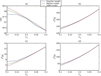
0.1 0.15 0.2 0.25 0.3 96
96.5 97 97.5 98 98.5
(a)
σA
C(0)
0.1 0.15 0.2 0.25 0.3 100
150 200 250 300
(b)
σA
V
P(0)
0.1 0.15 0.2 0.25 0.3 4
6 8 10 12 14
(c)
σA
V
R(0)
0.1 0.15 0.2 0.25 0.3 0
50 100 150 200
(d)
σA
V
D(0)
[image:17.612.128.470.90.349.2]Esscher model Merton model GBM model
Figure 1: Sensitivity of the overall policyholder’s claim and its component to the reference portfolio’s volatility.
computing the first three or four terms of the series. In this study, we consider the first 10 terms of the series in order to obtain a good approximation also when the parameter λ is allowed to change.
As far asVR(0) andVD(0) are concerned, they are obtained using Monte Carlo techniques. Precisely, we use standard Monte Carlo methods with 100,000 paths over 20 years. Each year includes 1 observation per month of the equity portfolio A; the returns are calculated annually. We use the antithetic variates methods for variance reduction purposes; we also make use of the closed form expressions for the values of the policy reserve as a control variate to reduce the variance of the estimates even further. In order to avoid the introduction of bias in the estimation, we use a few pilot runs to estimate the control variate parameter and then we use this estimate in the main sim-ulation run. The approximation error across the three models of the obtained estimates is then 0.008% for the value of the terminal bonus and 0.0006% for the value of the default option.
The solutions to equation (17) are then sought using the bisection method.
5.2
Numerical results
As panel (a) highlights, the values of the claimC obtained under the three models considered in this paper are very close (in fact the maximum mispricing generated by the geometric Brownian motion model is a 0.26% overpricing with respect to the ˆPM-measure based model and a 0.65% overpricing with respect to the Esscher model, both corresponding to σA = 10% p.a.).
The breakdown of C(0) into its building blocks, though, shows that this information is misleading. Panels (b)−(c)−(d), in fact, reveal that the geomet-ric Brownian motion-based model overestimates the value of the guaranteed benefits and the probability of default when compared to the ˆPM-measure based model. In other words, the classical Black-Scholes framework leads to a more prudential pricing rule, as it provides an upper bound for the value of the policy reserve and the default option. However, it underprices the value of the terminal bonus, i.e. it underestimates the capacity of the life insurance company for generating enough surplus to distribute to the policyholders. The maximum mispricing is 10.82%, again corresponding to σA = 10% p.a.
When compared with the valuation model based on the Esscher measure, instead, the standard Black-Scholes framework leads to the underpricing of the values of all the contract’s components. In particular, the biggest mispricing is, once again for σA = 10% p.a., 5% for the value of the policy reserve, 25% for the value of the terminal bonus and 18% for the value of the default option. Hence, reserving on the basis of the geometric Brownian motion model would lead us to set aside insufficient resources to cover the liabilities. Further, the assumption of a reference portfolio driven by a diffusion process would seriously underestimate the potential threat to the life insurance company solvency represented by the participating contract, as the higher risk of default would not be fully captured.
We also note the differences in the nature of the mispricing generated by the Black-Scholes framework with respect to the ˆPM-measure model and the Esscher measure paradigm, especially for the case of the default option, as
VD
M < VGBMD < VhD. This result could be explained by the fact that, differently from the pricing measure ˆPM, the Esscher measure does not preserve the val-uation approach’s independence of the investors’ risk preferences, which is one of the main features of the classical Black-Scholes model. In fact, as equation (A7) shows, the ˆPh-dynamic of the processLdepends on the parameterh solu-tion to the Esscher martingale condisolu-tion (11). In order to calculateh, we need to make some assumptions regarding the “real” drift of the L´evy process, i.e. the parameter a. Since the drift a represents the expected rate of growth of the reference portfolio, specifying an assumption for its value effectively means specifying the preferences structure of the investors. In this sense the Esscher measure can be seen as the closest probability to the real probability measureP
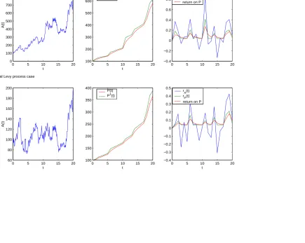
the Esscher measure appears to be the most suitable one to capture the ad-ditional risk induced by the occurrence of crashes in the market, as shown in Figure 2. In this Figure we represent two possible evolutions for the reference portfolio and the policy reserve. The first scenario is represented in the top three panels of Figure 2 and it is based on the geometric Brownian motion to model the asset backing the participating contract. At the expiration of the contract, the reference portfolio is worth £774 whilst the policy reserve has value £581. In this case the policyholder would be paid the guaranteed ben-efits in full. The second scenario, represented in the bottom panels of Figure 2, uses the same set of random numbers to generate the diffusion part of the reference portfolio; however, on averageλ times per year the asset price jumps discretely of a random amount X. Since σA is kept constant, the final result is a higher instability of the rate of returns rA and rP to the extent that, at maturity, the portfolio is worth£183 against the£367 liability represented by the policy reserve. In this case the life insurance company would default.
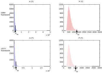
The instability produced in the model by the jump component is also il-lustrated in Figure 3, in which we show how the probability of default changes under both the Brownian motion and the L´evy process paradigm, when the total volatility σA is allowed to change, and in Figure 4, in which, instead, we represent the distributions of the asset and the policy reserve under both market’s paradigm. The last Figure, in particular, shows the 99% percentile of the policy reserve distribution; the probability thatA(T) is less than this 99% percentile is 73% in the geometric Brownian motion-based model, and 86% in the L´evy process-based model.
The effects on the fair combinations of the design parameters β and rG produced by the inclusion of jumps in the market model are represented in Figure 5. Here we show that the additional jump feature restricts the set of optimal choices for the participation rate β. In particular, in panel (a), we represent the values that the parameter β is allowed to assume in order to satisfy equation (17) when σA changes. The optimal β set is smaller in the case of the Esscher valuation framework because of the higher default risk that characterizes this model, as already discussed earlier. Although the geometric Brownian motion overprices the value of the claims with respect to the PM measure, the participation rate β is set at a lower level in the PM -based paradigm than in the geometric Brownian motion one. This fact is due to the higher rates of increase of the value of the default option induced by the same increase in σA, that characterizes the PM model. Panel (c) shows that, the reference portfolio’s volatility σA being equal, the set of fair values for the participation rate β becomes even smaller when the jumps are allowed to occur more often, i.e. when the market becomes more unstable. The reason is again to be sought for in the impact of higherλ on the default risk attached to the participating contract.
0 5 10 15 20 0 100 200 300 400 500 600 700 800 900 t A(t)
0 5 10 15 20
100 200 300 400 500 600 700 t P(t) P1(t)
0 5 10 15 20
−0.4 −0.2 0 0.2 0.4 0.6 0.8 1 r A(t) r P(t)
return on P
0 5 10 15 20
60 80 100 120 140 160 180 200 A(t) t
0 5 10 15 20
100 150 200 250 300 350 400 t P(t) P1(t)
0 5 10 15 20
−0.4 −0.3 −0.2 −0.1 0 0.1 0.2 0.3 0.4 0.5 t r A(t) r P(t)
return on P The geometric Brownian motion case
The general Levy process case
[image:20.612.177.664.126.480.2]0.1 0.15 0.2 0.25 0.3 0.35 0.4 0.45 0.5 0
0.1 0.2 0.3 0.4 0.5 0.6 0.7 0.8 0.9
σA
P(A(T)<P(T))
Levy framework
[image:21.612.129.468.93.343.2]GBM framework
Figure 3: Default probabilities in the two market paradigm presented in the paper and their sensitivity to the reference portfolio volatility.
0 1 2 3 4 5
x 104 0
1000 2000 3000 4000 5000 6000
A (T)
0 500 1000 1500 2000 2500 3000 3500 0
200 400 600 800 1000 1200
0 0.5 1 1.5 2 x 10⁴ 0
1000 2000 3000 4000
0 500 1000 1500 2000 2500 3000 0
200 400 600 800 1000 1200 GBM
framework
LEVY framework
A (T)
P (T)
P (T) P99 P
99
P99 P
99
[image:21.612.123.470.403.654.2]0.1 0.14 0.18 0.22 0.26 0.3 0.76
0.78 0.8 0.82 0.84 0.86 0.88 0.9 0.92 0.94
C(0) = P
0
σA
β
0.1 0.120.140.160.18 0.2 0.220.240.260.28 0.3 0.2
0.3 0.4 0.5 0.6 0.7 0.8 0.9 1
(b)
σA
r G
0.5 0.65 0.8 0.95 1.1 1.25 1.4 1.55 1.7 1.85 2 0.68
0.72 0.76 0.8 0.84 0.88 0.92
(c)
λ
β
0.5 0.6 0.7 0.8 0.9 1 1.1 1.2 0.35
0.4 0.45 0.5 0.55 0.6 0.65 0.7 0.75 0.8 0.85 0.9 0.95 1
(d)
λ
r G
(a)
GBM model
Merton model
Esscher model
GBM model
GBM model
GBM model Merton model
Merton model
Merton model Esscher model
Esscher model
[image:22.612.127.469.86.346.2]Esscher model
Figure 5: Isopremia curves: the fair set of the participation rateβ and the guaran-teed rate rG against the portfolio volatility σAand the jump’s frequency λ.
performed under the PM and the Ph measures, also explains the higher levels of the guarantee rG needed to maintain the fairness of the contract, as shown in both panels (b) and (d). The policyholder, in fact, will ask for a bigger guaranteed fixed benefit as a compensation for the higher risk contained in the contract. Panel (b), though, shows that rG needs to be reduced when the market is very volatile in order to control better the exposure to the default risk. On the other hand, panel (d) shows that,σAbeing equal, the policyholder will seek increasingly higher levels ofrG if he/she has the feeling that the value of the portfolio is subject more frequently to possible crashes. Note that in the PM-based paradigm and in the Esscher framework, no solution is possible when more than one jump every 10 months and every 14 months respectively is expected (corresponding to the values ofλequal to 1.2 and 0.9 respectively).
6
Concluding remarks
This study finds its justification in the new recommendations from the IASB and the financial authorities to adopt adequate models for both the dynamic of the asset prices and the calculation of life insurance companies’ liabilities. The recent literature has addressed so far only the problem of the implementation of suitable fair valuation techniques for participating con-tracts. However, the results presented in this paper show the importance of modelling the asset side as well of the company’s balance sheet, in order to properly assess market risks, and their impact on the value of these contracts and the company’ solvency. As shown in section 5, in fact, mispecifying the underlying process driving the asset prices, can lead to underestimating the insurance company’s risk of default, and consequently setting aside insufficient resources.
We note that the alternative asset price process used in this study is a L´evy process with finite activity, i.e. a process which can be decomposed as the sum of a Brownian motion with drift (the diffusion part) and a compound Poisson process (the jump part), as in Merton (1976). This form for the jump-diffusion process has considerable intuitive appeal as it can be regarded as mirroring the nature of the information flow from the market. This flow, in fact, is seen as given by a sort of basic information of an “ordinary” kind causing only marginal changes in prices, in addition to which there is also information of a very important nature, originating abnormal movements in market prices. The former can be interpreted as a continuous motion, like a diffusion process, whilst the latter can be regarded intuitively as a compound Poisson process since, by its very nature, important information arrives only at discrete points in time. A recent analysis offered by Carr et al. (2002), however, shows that in general market prices lack of a diffusion component, as if it was diversified away. Carr et al (2002), hence, conclude that there is an argument for using pure jump processes of infinite activity and with finite variation, given their ability to capture both frequent small moves and rare large moves. Processes of this kind extensively used in finance are the variance gamma (VG) process (Madan et al., 1990, 1991, 1998) and the CGMY process (Carr et al., 2002).
be reasonable for derivatives actively traded in the market, its application to the (fair) valuation life insurance liabilities might prove unsatisfactory for the lack of suitable exchange prices. On the basis of the definition of fair value provided by IASB, the “price” of an insurance liability should not be different from the market value of a portfolio of traded assets matching the liability cas-flows with sufficient degree of certainty. However, such traded assets are not easy to identify mainly due to the long time horizons covered by participating contracts, but also due to the mortality risk that in general affects these con-tracts (and that we ignore in this paper). Alternatively, the required exchange prices could come from secondary markets where (re)insurers can exchange “books” of policies, although these kinds of markets are not fully developed at the moment. Moreover, the statistical martingale measure approach might suf-fer from the same potentially serious problem affecting any parametric model. In fact, as Stanton (1997) observes, fitting historical data well is no guarantee of matching, over the required time horizon, the entire distribution of future prices (upon which the current value of the contingent claim depends), leading to the possibility of large pricing and hedging errors. A possible solution to this problem might rely on possible links between the structure of investors’ risk preferences, indices of risk aversion and the expected rate of growth of the underlying asset. We leave this question for future research.
A
Distribution properties of
L
(
t
)
under
P
ˆ
In section 3, we specified the L´evy decomposition to be:
L(t) =at+σW (t) +
Z t
0
Z
R
x(N(ds, dx)−ν(dx)ds).
Hence, the L´evy-Khintchine formula implies that the moment generating func-tion of the process L can be written as
EekL(t)
=etϕ(k)
where
ϕ(k) = ak+ σ
2
2 k
2+
Z
R
ekx−1−kxν(dx). (A2)
In particular, under the risk-neutral martingale measure ˆP, the moment gen-erating function will take the form
ˆ
EekL(t)
= etϕˆ(k),
ˆ
ϕ(k) = Ak+Γ
2
2 k
2+
Z
R
The aim of this section is to determine the functionsA, Γ and ˆν, i.e. the char-acteristic triplet of the semimartingale L, under the two alternative martingale measures considered in this paper, using the fact that
ˆ
EekL(t) =Eη(t)ekL(t),
where η(t) is the density process defined in section 4.
Let’s consider the case of the Merton measure first. As discussed in section 4.1, the Radon-Nikod´ym derivative for the probability ˆPM is
η(t) =e−GW(t)−G22t. Hence
ˆ
EekL(t)
= Ehe−GW(t)−G22tek(at+σW(t)+Rt
0
R
Rx(N(ds,dx)−ν(dx)ds))
i
= etϕˆM(k),
with
ˆ
ϕM(k) = (a−σG)k+
σ2
2 k
2+
Z
R
ekx−1−kx
ν(dx). (A3) Therefore, the characteristic triplet is:
A=a−σG; Γ =σ; ˆν(dx) = ν(dx).
This implies that under ˆPM the decomposition of the process L is
L(t) = (a−σG)t+σWˆM(t) +
Z t
0
Z
R
x(N(ds, dx)−ν(dx)ds).
The martingale condition (7) implies
L(t) =
r−σ
2
2 −
Z
R
(ex−1)ν(dx)
t+σWˆM(t) +
Z t
0
Z
R
xN(ds, dx). (A4)
Equations (A3) and (A4) imply that ˆWM is a standard one-dimensional ˆPM -Brownian motion, whilst the ˆPM-law of the compound Poisson process is the same as the one under the real probability measure P.
Moreover,
ˆ
EM
ekL(t)|N(t) =n
= ek
r−σ22−RR(ex−1)ν(dx)t+σ2
2 k2tEˆ
M
h ekR0t
R
RxN(ds,dx)
N(t) =n i
= ek
r−σ22−R
R(e
x−1)ν(dx)t+σ2
2 k2tEˆ
M ekx
n
;
since X ∼N(µX, σ2X), then
ˆ
EM
ekL(t)|N(t) =n
=ek
r−σ22−R
R(e
x−1)ν(dx)t+nµ X
+k2
Equation (A4) is used in section 5 to implement the Monte Carlo procedure for the valuation of terminal bonus and the default option. Equation (A5) is instead used in section 4.1 to calculate the value of the policy reserve.
Analogous calculations can be carried out for the case of the Esscher mea-sure ˆPh. In this case, the Radon-Nikod´ym derivative is defined as
η(t) =ehL(t)−tϕ(h).
Comparing the above expression of the process η to the more general one provided in section 4, we deduce that G(t) = −σh and H(t, x) = ehx. The moment generating function of the L´evy process is given by
ˆ
Eh
ekL(t) = e−tϕ(h)Ee(h+k)L(t)
= ek(a+σ2h)t+σ
2 2 k2t+t
R
R(e
hx(ekx−1)−kx)ν(dx)
= ek(a+σ2h−RRxν(dx)+ R
Rxe
hxν(dx))t+σ2
2 k2t+t
R
R(e
kx−1−kx)ehxν(dx)
= etϕˆh(k)
with
ˆ
ϕh(k) =
a+σ2h− Z
R
xν(dx) +
Z
R
xehxν(dx)
k+σ
2
2k
2+
Z
R
ekx−1−kxνˆ(dx).
(A6) This implies that the ˆPh-characteristic triplet is:
A=a+σ2h−RRxν(dx) +R
Rxe
hxν(dx) ; Γ =σ; ˆν(dx) = ehxν(dx). Bearing in mind that hsolves the Esscher martingale condition (11), it follows that the corresponding decomposition of the process L is then:
L(t) =
r− σ
2
2 −
Z
R
ehx(ex−1)ν(dx)
t+σWˆh(t) +
Z t
0
Z
R
xN(ds, dx).
(A7) Equations (A6) and (A7) imply that, under ˆPh,Wˆhis a standard one-dimensional Brownian motion, and the compound Poisson process Rt
0
R
RxN(ds, dx) has
compensator measure ˆν(dx) = ehxν(dx). Therefore, the ˆ
Ph-rate of the Pois-son process N is
λh =λehµX+h
2σ2X
2 ,
whilst the ˆPh-distribution of the jump random sizeX isN(µX +hσX2, σX2). In fact:
ˆ
Ph[N(t) =n] = ˆEh
1(N(t)=n)
=Eη(t) 1(N(t)=n)
= ML(h,1)−tE
ehL(t)|N(t) =n
P[N(t) =n] = P[N(t) =n]
ML(h,1) t e
ha−R
Rxν(dx)+
σ2
2 h
t+nhµX+nh2 σX2
Let
µh =ehµX+h
2σ2X
2 ,
then
ˆ
Ph[N(t) =n] =P[N(t) =n]enlnµh−λt(µh−1). (A8) Therefore
ˆ
Ph[N(t) =n] =
e−λht(λ
ht)n
n! . Moreover
ˆ
Eh
h ekR0t
R
RxN(ds,dx)
i
= e h
a−R
Rxν(dx)+
σ2
2 h
t
ML(h,1)t
E
h
e(h+k)R0t
R
RxN(ds,dx)
i
= et
R
R(e
kx−1)ehxν(dx)
.
Since, under the real probability measure P, X ∼ N(µX, σX2) and ν(dx) =
λf(dx), then
ˆ
Eh
h ekR0t
R
RxN(ds,dx)
i
=e
λht
e
k(µX+hσX2)+k 2σ2
X
2 −1
.
On the other hand, the moment generating function of a compound Poisson process has form:
ˆ
Eh
h ekR0t
R
RxN(ds,dx)
i
=eλht(Eˆh(ekx)−1),
which implies that
ˆ
Eh ekx
=ek(µX+hσ2X)+ k2σX2
2 .
Finally, we can also calculate the conditional moment generating function of the process L, which returns
ˆ
Eh
ekL(t)|N(t) =n=ek
r−σ22−R
Re
hx(ex−1)ν(dx)t+σ2
2 k2tEˆ
h ekx
n . Hence ˆ Eh
ekL(t)|N(t) =n=ek
r−σ22−R
Re
hx(ex−1)ν(dx)t+nµ
X+nhσ2X
+k22(σ2t+nσ2
X).
(A9)
B
Valuation using the Merton measure
Equation (8) in section 4.1 shows that the one-year call option embedded in the policy reserve has value
ˆ
EM
e−rβeL′(1)
−(β+rG)
+
= ˆEM
ˆ
EM
e−rβeL′(1)
−(β+rG)
+
N′
(1) =n
Since, as shown in the previous section, conditioning on the number of jumps occurring in one year
L(t)−L(t−1)∼N
rn−
v2n 2 , v
2
n
,
then the inner expectation can be written as
ˆ
EM
e−rβeL′(1)−(β+rG)
+
N′(1) =n
= ˆEM
" e−r
βern−v
2
n
2 +vny −(β+rG)
+# ,
where y∼N(0,1). Therefore
ˆ
EM
" e−r
βern−
vn2
2 +vny
−(β+rG)
+#
= ˆEM
βe−r+rn−v
2
n
2 +vny1
βern−v 2
n
2 +vny>β+rG
!
−e
−r
(β+rG) ˆPM
βern−v
2
n
2 +vny > β +rG
= βe−r+rn
Z ∞
a 1 √
2πe
−(y−2vn)2
dy−e−r(β+rG) ˆPM (y > a),
with
a= ln β+rG
β −
rn−
v2 n 2 vn . Hence ˆ EM " e−r
βern−v
2
n
2 +vny−(β+rG)
+#
=βe−r+rnN(d
n)−e−r(β+rG)N(d′n), (B1) with
dn =
lnβ+βr
G +
rn+ v
2 n 2 vn ; d′
n = dn−vn. Since
rn=r−λ(µ−1) +nlnµ, we can rewrite equation (B1) as
βe−λ(µ−1)+nlnµN
(dn)−e−r(β+rG)N(d′n) = e−λ(µ−1)+nlnµf(n),
where
References
[1] Bacinello, A. R. (2001). Fair pricing of life insurance participating con-tracts with a minimum interest rate guaranteed.Astin Bulletin, 31, 275-97.
[2] Bacinello, A. R. (2003). Pricing guaranteed life insurance participating policies with annual premiums and surrender option. North American Actuarial Journal, 7 (3), 1-17.
[3] Bakshi, G. S., Cao, C. and Chen, Z. (1997). Empirical performance of alternative option pricing models, Journal of Finance, 52, 2003-49.
[4] Ballotta, L., Haberman, S. and Wang, N. (2004). Guarantees in with-profit and unitised with with-profit life insurance contracts: fair valuation problem in presence of the default option, to appear in Journal of Risk and Insurance.
[5] Black, F. and Scholes M. (1973). The pricing of options on corporate liabilities, Journal of Political Economy, 81, 637-59.
[6] Brennan, M. J. and Schwartz E. S. (1976). The pricing of equity-linked life insurance policies with an asset value guarantee,Journal of Financial Economics, 3, 195-213.
[7] Carr, P., Geman. H., Madan D. B. and Yor M. (2002). The fine structure of asset returns: an empirical investigation, Journal of Business, 75, 305-32.
[8] Chan, T. (1999). Pricing contingent claims on stocks driven by L´evy pro-cesses, The Annals of Applied Probability, 9, 504-28.
[9] Cummins, J. D., Miltersen K. R. and Persson S. V. (2004). In-ternational comparison of interest rate guarantees in life insurance, XXXVthInternational Astin Colloquium, Bergen.
[10] Eberlein, E., Keller U. and Prause K. (1998). New insights into smile mispricing and value at risk: the hyperbolic model. Journal of Business, 71, 371-405.
[11] Esscher, F. (1932). On the probability function in the collective theory of risk,Skandinavisk Aktuarietidskrift, 15, 175-95.
[12] Fama, E. (1965). The behaviour of stock market prices, Journal of Busi-ness, 38, 34-105.
[14] Gerber, H. U. and Shiu E. S. W. (1994). Option pricing by Esscher trans-forms (with discussion), Transactions of the Society of Actuaries, 46, 99-140; discussion: 141-91.
[15] Grosen, A. and Jørgensen P.L. (2000). Fair valuation of life insurance liabilities: the impact of interest rate guarantees, surrender options, and bonus policies, Insurance: Mathematics and Economics, 26, 37-57.
[16] Grosen, A. and Jørgensen P. L. (2002). Life insurance liabilities at mar-ket value: an analysis of investment risk, bonus policy and regulatory intervention rules in a barrier option framework.Journal of Risk and In-surance, 69, 63-91.
[17] Guill´en M., Jørgensen P.L. and Perch-Nielsen J. (2004). Return smooth-ing mechanism in life and pension insurance: path-dependent contsmooth-ingent claims, Working Paper.
[18] Haberman, S., Ballotta L. and Wang N. (2003). Modelling and valuation of guarantees in with-profit and unitised with profit life insurance con-tracts, Actuarial Research Paper N. 146, City University London, under review.
[19] Jacod, J. and Shiryaev A. N. (1987). Limit Theorems for Stochastic Pro-cesses, Springer-Verlag.
[20] Jarrow. R. and Rosenfeld E. (1984). Jump risks and the intertemporal capital asset pricing model, Journal of Business, 57, 337-51.
[21] Madan, D. B., Carr P. and Chang E. (1998). The variance gamma process and option pricing, European Finance Review, 2, 79-105.
[22] Madan, D. B. and Milne F. (1991). Option pricing with VG martingale components, Mathematical Finance, 1, 39-45.
[23] Madan, D. B. and Seneta E. (1990). The variance gamma (VG) model for share market returns.Journal of Business, 63, 511-24.
[24] Mandelbrot, B. (1963). The variation of certain speculative prices,Journal of Business, 36, 394-419.
[25] Merton, R. C. (1973). Theory of rational option pricing, Bell Journal of Economics, 4, 141-83.
[27] Miltersen, K., R. and Persson S. A. (2003). Guaranteed investment con-tracts: distributed and undistributed excess return, Scandinavian Actu-arial Journal, 23, 257-79.
[28] Nahum, E. (1998). On the distribution of the supremum of the sum of a Brownian motion with drift and a marked point process, and the pricing of lookback options, Technical Report N◦ 516, Department of Statistics,
University of California, Berkeley.
[29] Needleman, P. D. and Roff T. A. (1995). Asset shares and their use in the financial management of a with-profits fund,British Actuarial Journal, 1, IV, 603-88.
[30] Stanton, R. (1997). A nonparametric model of term structure dynamics and the market price of interest rate risk, The Journal of Finance, 52, 1973-2002.