Efficient and Robust Segmentations Based on Eikonal and Diffusion PDEs

City, University of London Institutional Repository

Citation

:

Peny, B., Unal, G. B., Slabaugh, G. G., Fang, T. and Alvino, C. V. (2006).

Efficient and Robust Segmentations Based on Eikonal and Diffusion PDEs. In: Zheng, N,

Jiang, X and Lan, X (Eds.), Advances in Machine Vision, Image Processing, and Pattern

Analysis. Lecture Notes in Computer Science, 4153. (pp. 339-348). Springer. ISBN

3-540-37597-X

This is the accepted version of the paper.

This version of the publication may differ from the final published

version.

Permanent repository link:

http://openaccess.city.ac.uk/4414/

Link to published version

:

http://dx.doi.org/10.1007/11821045_36

Copyright and reuse:

City Research Online aims to make research

outputs of City, University of London available to a wider audience.

Copyright and Moral Rights remain with the author(s) and/or copyright

holders. URLs from City Research Online may be freely distributed and

linked to.

Efficient and Robust Segmentations Based on Eikonal

and Diffusion PDEs

Bertrand Peny, Gozde Unal, Greg Slabaugh, Tong Fang1and Christopher Alvino2

1

Intelligent Vision and Reasoning Siemens Corporate Research

Princeton NJ 08540, USA 2

Section of Biomedical Image Analysis Department of Radiology University of Pennsylvania Philadelphia PA 19104, USA

Abstract. In this paper, we present efficient and simple image segmentations

based on the solution of two separate Eikonal equations, each originating from a different region. Distance functions from the interior and exterior regions are computed, and final segmentation labels are determined by a competition crite-rion between the distance functions. We also consider applying a diffusion partial differential equation (PDE) based method to propagate information in a manner inspired by the information propagation feature of the Eikonal equation. Experi-mental results are presented in a particular medical image segmentation applica-tion, and demonstrate the proposed methods.

1

Introduction

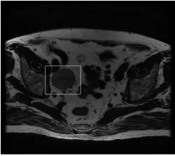
Content extraction from images usually relies on a segmentation, i.e., extraction of the borders of target structures. Accurate segmentation may be hampered by noise in the image acquisition, the complexity of the arrangement of the target objects with respect to the surrounding structures, and the computational cost of the algorithm used. In this study, a new algorithm to segment the boundary of a closed structure is developed based on ideas of propagation and diffusion of image information. Our work is motivated by anatomical structures such as lymph nodes, (see Figure 1), whose extraction from medical images, such as Magnetic Resonance (MR) images, is an important task for subsequent quantitative analysis. Clinically useful segmentations should be fast and accurate, so that quick and precise interpretation of the anatomical structures can be obtained.

is different. Although we also make use of two distance maps, we do not need to extract a minimal path through a back-propagation from the point where the two fronts meet, but we seek for the result of the competition of the two fronts in reaching a given point. Similarly, Cohen et al. [2, 3] used a fast marching algorithm for segmenting tubular structures like vessels, incorporating geodesic distance of the points on the propagation path to the seed point as a freezing measure. Similarly, a multiphase fast marching al-gorithm was utilized in [4], where all distinct regions are propagated simultaneously according to their respective velocities, which depend on posterior probability densities of each region.

There are also similarities between watershed algorithms and the fast marching al-gorithms. The Eikonal PDE has been used in [5] for modeling watershed segmentation that is constructed by flooding the gradient image. Different segmentation results have been obtained by changing the flooding criteria [6] such as constant height, area or volume. A form of diffusion has been used for image segmentation in [7] by a random-walker concept. This technique differs from our approach in that it was introduced in a graph theoretic framework [8], and formulated as a linear system of equations solved through conjugate gradients.

In this paper we present four methods. The first three methods compute distance functions treating image edge or image gradient information as locally slower to prop-agate information or as high local distance. These three methods employ the Eikonal equation and thus can be computed rapidly by the fast marching algorithm. Inspired by the same distance ideas, we also present a fourth method based on diffusion PDEs, in which edge information is propagated from the interior or exterior of the structure.

Fig. 1. Example of an MR image with a region of interest (ROI) around a lymph node.

2

Segmentation by Interior/Exterior Distance Competition

3

For instance a rectangular region of interest (ROI), completely surrounding the desired structure, whose borders are exterior points and center are interior points, can be se-lected. The local distance depends on the image intensity variation of the region that we want to segment. Regions that are more likely to be edges should be interpreted as regions in which distance information propagates more slowly. This idea will be imple-mented in several different ways. In the first, we weight the distance function directly on the binary map resulting from an edge detection on the image, for instance using a Canny edge detector. Edges in the edge map correspond to obstacles when the distance function is computed. The second method generalizes the first method, by defining the local distance as the gradient magnitude of the image. The third method combines the different weights on the distance function. The fourth method in inspired by distance propagation ideas and uses a diffusion PDE as will be explained.

The first three methods comprise a propagation of information using a weighted shortest distance, they can be implemented by solving an Eikonal PDE. To achieve fast computation of the two different distance functions, we used the fast marching algo-rithm. Our fourth idea requires a diffusion PDE as we will explain. The next subsec-tions describe briefly the fast marching algorithm, how to adapt it to fit our ideas, and the diffusion method.

2.1 Method

The fast marching algorithm [9] is designed to compute the position of a propagating front with position varying speed given by the function F>0. Let a functionD :Ω∈

Rn_{−→Rdescribe the arrival time of the front when it crosses each pixel (x,y), where}

n = 2 for an image function,n = 3for an image volume. Fast marching solves the Eikonal equation which can be represented by

|∇D|=F, D= 0on G

whereGis a prespecified subset ofRn_.

If the speed functionFis constant, thenDrepresents the distance function toG. In our segmentation method the speed of the motion will be selected differently based on intensity variation as explained previously.

Our method proceeds as follows:

1. Compute the two distance functions: one for the interior by settingG=Diand the other for the exterior by settingG=Deneeded in our segmentation algorithm. 2. Set up the image information propagation algorithm either through a propagation

operation with fast marching or through a diffusion equation. The starting points set are the set of seeds, which we are sure that they belong to the background that surrounds the structure to segment (Known points). These are the boundary conditions for both the Eikonal PDE and the diffusion PDE.

The Eikonal PDE:

– Exterior: Run the fast marching algorithm by computing theL1distances with specific weights as will be explained in the next subsections. The value of each pixel then corresponds to the distance to the exterior set and is denoted asDe. – Interior: Run the fast marching a second time for the interior set to obtain dis-tance functionDi_{. The method starts this time with interior points as Known}

set.

Similarly, the diffusion PDE is solved twice with two different set of boundary conditions to obtain two distance functionsDi_andDe_{at its steady state solution.}

3. The region interior is considered the set of points where the interior distance is less than the exterior distance, i.e.,{(x, y) :Di(x, y)< De(x, y)}

The different weights of the distance function as well as the diffusion are explained in the following sub-sections.

2.2 Fast Marching with Edge Map

Our first approach is to compute the distance function where edge pixels represent points where the information is propagated slowly in the shortest path between a pixel and the starting set of points,G. The Eikonal equation then transforms to:

|∇D|= (1 +Edge Map). (1)

Any edge detection algorithm with binary output can be used to obtain the edge map. In our results, we use a Canny edge detector. In the fast marching algorithm the edge pixels are marked as having infinity as their initial distance and are labeled as known. In this way they will not be processed during the distance function computation. The first column in Figure 2 depicts the two distance functions computed by starting from both the interior and the exterior seed points.

2.3 Fast Marching with Gradient

In the second method, we treat regions with high gradient magnitude as having high local distance, and regions with low gradient magnitude as having low local distance. The Eikonal equation then takes the form:

|∇D|= (|∇I|) (2)

The second column in Figure 2 depicts the two distance functions computed in this way.

2.4 Diffusion Equation

The linear heat equation on a functionDis given by dD_dt =∆Dwith initial conditions D(x, y)|t=0 =D0(x, y). A finite difference approximation to this equation forn= 2, that is obtained by implementing a forward Euler numerical scheme with the maximally stable time step is,

D(x, y) =1

4D(x+ 1, y) + 1

4D(x−1, y) +1

4D(x, y−1) + 1

5

Fig. 2. Rows 1. Interior distance; 2. Exterior distance function. Columns 1. with edge map; 2.

with gradient; 3. with diffusion.

hence diffusing edge information from the boundaries towards the non-boundary re-gions.

Inspired by the Eikonal equation and fast marching techniques, where we propagate the information from the boundaries or the seeds of the domainΩtowards unlabeled points, diffusion equations can also be utilized for segmentation with a similar twist for creating two smooth distance functions for the interior seeds and the exterior seeds. To introduce image dependent terms to the diffusion equation, our intuition is that the diffusion takes the path of least resistance, that is the path where the one-sided image gradient in a given direction is low. The definition of the four one-sided image gradients or sub-gradients around a pixel are given by

Ix−(x, y) =I(x, y)−I(x−1, y), Ix+(x, y) =I(x+ 1, y)−I(x, y)

I−

y(x, y) =I(x, y)−I(x, y−1), Iy+(x, y) =I(x, y+ 1)−I(x, y)

We can create an based discrete diffusion equation by introducing the image-driven weights to the discrete Laplacian equation as follows,

D(x, y) = w

E P

wiD(x+ 1, y) +

wW P

wiD(x−1, y)

+ w

N P

wiD(x, y−1) +

wS P

wiD(x, y+ 1), (4)

wE_=e−β(I+

x)2, wW =e−β(Ix−)2,

wN _=e−β(I−

y)2, wS =e−β(Iy−)2, i∈ {E, W, N, S}.

This image-weighted diffusion we seek for our distance functionD is similar in spirit but also quite different in the basic idea and the application from the work of Perona-Malik et al. [10] who used anisotropic diffusion for filtering images respecting image gradient directions. Using a similar weighted diffusion equation based on image gradients∂I/∂t=∇ ·(w(|∇I|)∇I), they actually solve for the image functionInot the distance functionDas we do.

2.5 Combined Method

In the second method explained in Section 2.3, which uses the gradient magnitude as the local distance function, we found some cases where the algorithm leaked. This is partly explained by the fact that for some interior regions, their edges are quiet weak, so the gradient is lower as expected. To prevent those leaks and increase robustness, one can combine the first two methods in Section 2.2 and 2.3. This corresponds to weight the distance function also by edge information. The method consists of first computation of the edge map as explained before to result in a binary image of the ROI. This binary image is then directly added to the gradient image by a factorα. The Eikonal equation then takes the form:

|∇D|= (|∇I|+α∗E), (5)

where E is the binary edge map. This will result in increased gradient effects where there are edges.

The algorithm described is very flexible in that it is possible to have different dis-tance functions for the foreground and background set of points. This flexibility may help for segmentation of textured interior regions for example. One can add, to the foreground distance function, some interior intensity information, which will smooth the local gradient and decrease some texture or noise influence. We do not smooth the background distance function, because exterior region may include other structures. The idea is to compute the mean intensity of the foreground set of points, sayImean.

The image at each pixel p will then have a local weight of(I[p]−Imean)2, which we

add to the foreground Eikonal equation by a factorβ:

¯

¯_∇Di¯_¯=³_{|∇I|+α∗E+β∗(I−I}

mean)2

´

, (6)

where E is the binary edge map andImean is the mean intensity of the foreground set

of points.

3

Results and Conclusions

7

implementation. Although we extended the diffusion approach to 3D as well, the com-putation times increased to order of 1 to 2 minutes, therefore, we have not utilized the diffusion-based approach for the 3D experiments.

Placement of interior and exterior seeds is flexible, and can be done by for instance a mouse brush. However, we opted a simple mouse drag operation on an image slice that sets exterior seeds in the form of a 2D rectangular border, then the interior seeds are automatically set to the set of pixels in the center of this rectangle. This type of 2D initialization is used in our both 2D and 3D experiments.

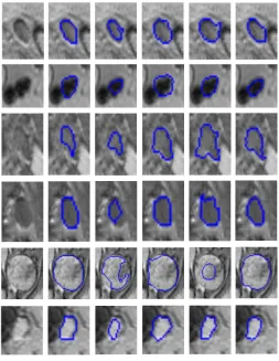
In Figure 3, sample segmentation results (labeled as blue contours) are presented for lymph node structures in MR images under different situations. By analyzing the results based on the edge map algorithm, in some cases the segmentation is not as precise as the other methods. The Canny edge detector propagates strong edges and discards the weak ones, and this leads to either edge noise (row 3, 4 and 5), or “holes” in the edge map (row 1). This will influence directly the distance functions and in turn the final seg-mentation. Still the result can be acceptable as an initialization to a more sophisticated segmentation algorithm. Those errors are reduced by our second approach that uses image gradient in the Eikonal PDE. The distances found are then smoother, and our segmentation matches the node contour better. In cases where a strong edge is situated near the node contour, the gradient method may be slightly attracted to it (rows 1 and 5), and comes from the fact that the gradient is a local intensity variation characteristic. Despite small incoherences, the results have very good quality. Finally the diffusion method performs well in strong edge neighborhoods, but easily smears the information when objects are merged, hence obtains a mid-way distance estimation (rows 1 and 3 in Fig. 3). This can be explained by the fact that the algorithm is based on a diffusion of in-tensity variation around pixels, so merged structures will affect the segmentation more than other structures in the neighborhood of the node. Finally our combined method optimizes the results, in difficult nodes. The edge information restrains the leak that we could see in the gradient method, for example row 3 and 5 in Fig. 3.

The results are confirmed by the statistics we found during our tests(see Table 1). We compute the mean of falsely rejected pixels (Type II error) and falsely accepted pixels (Type I error) on the resulting contours of the presented four segmentation meth-ods compared with the manually delineated node contours. The very low value in the Type I error of the edge map method is explained by its conservative behavior due to binary edge information onto which the propagating front can get stuck. This implies that we missed part of the interior area, hence a high value for the Type II error. On the other hand the Gradient and Diffusion methods are more prone to leaks and have then a higher Type I error. Finally the combined method is a good compromise between leaking and conservative error. Of course this appreciation depends on how we want to use the segmentation and we may prefer one algorithm over another because of its evolution characteristics. We want to note that the ground truth of each node was drawn using a mouse and by our own learned interpretation from clinicians,where the bound-aries should be, this may then cause some result discrepancies due to imprecisions.

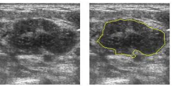
We perform the segmentation also on other type of images, like for example in Fig. 5 on Computed Tomography (CT) sequences to segment a tumor in the liver as shown on the right. The 3D tumor extraction results are shown in Fig. 6. The Fig. 7 is an example of a breast mass segmentation in an ultrasound image. As we can see, ultrasound images have speckle noise, that hampers segmentation, therefore we had to pre-process the image with high level of smoothing, to reduce it. The results show that our algorithm works for different types of images and may be tuned for applications other than lymph node segmentation.

In conclusion, we presented efficient and simple image segmentations based on ideas from the Eikonal and diffusion PDEs, by computing the distance functions for the exterior and interior regions, and determining the final segmentation labels by a competition criterion between the distance functions for reaching a given point. Each method has its pros and cons, according to the image characteristics, but our exper-iments demonstrated that among the presented methods, the combined fast marching method achieved a better speed vs. accuracy ratio, hence the best utility when com-pared to the other three methods.

Acknowledgements

We thank Dr. M. Harisinghani, Dr. R. Weissleder at Massachusetts General Hospital (MGH) in Boston, Dr. J. Barentsz at University Medical Center in Nijmegen, Nether-lands, for clinical motivation, feedback and providing data, and Dr. R. Seethamraju for discussions, Dr. R. Krieg at Siemens Medical Solutions for support of this work.

References

1. Deschamps, T., Cohen, L.D.: Fast extraction of minimal paths in 3d images and applications to virtual endoscopy. Medical Image Analysis 5 (2001)

2. Deschamps, T., Cohen, L.D.: Fast extraction of tubular and tree 3d surfaces with front prop-agation methods. ICPR (2002)

3. Cohen, L.D., Kimmel, R.: Global minimum for active contour models: A minimal path approach. IJCV (1997)

4. Sifakis, E., Garcia, C., Tziritas, G.: Bayesian level sets for image segmentation. J. Vis. Commun. Im. Repres. (2001)

5. Meyer, F., Maragos, P.: Multiscale morphological segmentations based on watershed, flood-ing, and eikonal pde. Proc. Scale-Space (1999) 351–362

6. Sofou, A., Maragos, P.: Pde-based modeling of image segmentation using volumic flooding. ICIP (2003)

7. Grady, L., Lea, G.: Multi-label image segmentation for medical applications based on graph-theoretic electric potentials. In: ECCV, Workshop on MIA and MMBIA. (2004)

8. Boykov, Y., Jolly, M.: Interactive graph cuts for optimal boundary and region segmentation of objects in n-d images. In: ICCV. Volume 1. (2001) 105–112

9. Sethian, J.: Level Set Methods and Fast Marching Methods. CUP (1999)

9

Fig. 3. Segmentation Results. Columns(a-f): a. ROI image; b. Node manually delineated; c. Edge

Map Method; d. Gradient Method; e. Diffusion Method, f. Combined Method.

Table 1. Error type I and II statistics over the Data Base (≈50 nodes)

Edge Map Method Gradient Method Diffusion Method Combined Method Type I 0.015 0.247 0.256 0.081 Type II 0.453 0.115 0.189 0.257

Fig. 5. A liver tumor is segmented using the Combined Algorithm on a CT volume.

Fig. 6. 3D Segmentation results on CT sequences of Fig. 5